A structured approach to proving compiler optimizations based on dataflow analysis

(1)

HAL Id: inria-00289549

https://hal.inria.fr/inria-00289549

Submitted on 21 Jun 2008

HAL is a multi-disciplinary open access

archive for the deposit and dissemination of

sci-entific research documents, whether they are

pub-lished or not. The documents may come from

teaching and research institutions in France or

abroad, or from public or private research centers.

L’archive ouverte pluridisciplinaire HAL, est

destinée au dépôt et à la diffusion de documents

scientifiques de niveau recherche, publiés ou non,

émanant des établissements d’enseignement et de

recherche français ou étrangers, des laboratoires

publics ou privés.

A structured approach to proving compiler

optimizations based on dataflow analysis

Yves Bertot, Benjamin Grégoire, Xavier Leroy

To cite this version:

Yves Bertot, Benjamin Grégoire, Xavier Leroy. A structured approach to proving compiler

optimiza-tions based on dataflow analysis. Types for Proofs and Programs, Workshop TYPES 2004, Dec 2004,

Jouy-en-Josas, France. pp.66-81, �10.1007/11617990�. �inria-00289549�

(2)

A structured approach to proving compiler

optimizations based on dataflow analysis

Yves Bertot1_{, Benjamin Gr´egoire}2_{, and Xavier Leroy}3

1

Projet Marelle, INRIA Sophia-Antipolis, France Yves.Bertot@sophia.inria.fr

2 _{Projet Everest, INRIA Sophia-Antipolis, France}

Benjamin.Gregoire@sophia.inria.fr

3

Projet Cristal, INRIA Rocquencourt, France Xavier.Leroy@inria.fr

Abstract. This paper reports on the correctness proof of compiler op-timizations based on data-flow analysis. We formulate the opop-timizations and analyses as instances of a general framework for data-flow analyses and transformations, and prove that the optimizations preserve the be-havior of the compiled programs. This development is a part of a larger effort of certifying an optimizing compiler by proving semantic equiva-lence between source and compiled code.

1 Introduction

Can you trust your compiler? It is generally taken for granted that compil-ers do not introduce bugs in the programs they transform from source code to executable code: users expect that the generated executable code behaves as prescribed by the semantics of the source code. However, compilers are complex programs that perform delicate transformations over complicated data struc-tures; this is doubly true for optimizing compilers that exploit results of static analyses to eliminate inefficiencies in the code. Thus, bugs in compilers can (and do) happen, causing wrong executable programs to be generated from correct source programs.

For low-assurance software that is validated only by testing, compiler bugs are not a major problem: what is tested is the executable code generated by the compiler, therefore compiler bugs should be detected along with program bugs if the testing is sufficiently exhaustive. This is no longer true for critical, high-assurance software that must be validated using formal methods (program proof, model checking, etc): here, what is certified using formal methods is the source code, and compiler bugs can invalidate the guarantees obtained by this certification. The critical software industry is aware of this issue and uses a variety of techniques to alleviate it, such as compiling with optimizations turned off and conducting manual code reviews of the generated assembly code. These techniques do not fully address the issue, and are costly in terms of development time and program performance.

It is therefore high time to apply formal methods to the compiler itself in order to gain assurance that it preserves the behaviour of the source programs.

(3)

Many different approaches have been proposed and investigated, including proof-carrying code [6], translation validation [7], credible compilation [8], and type-preserving compilers [5]. In the ConCert project (Compiler Certification), we investigate the feasibility of performing program proof over the compiler itself: using the Coq proof assistant, we write a moderately-optimizing compiler from a C-like imperative language to PowerPC assembly code and we try to prove a semantic preservation theorem of the form

For all correct source programs S, if the compiler terminates without errors and produces executable code C, then C has the same behaviour (up to observational equivalence) as S.

An original aspect of ConCert is that most of the compiler is written directly in the Coq specification language, in a purely functional style. The executable compiler is obtained by automatic extraction of Caml code from this specifica-tion.

In this paper, we report on the correctness proof of one part of the com-piler: optimizations based on dataflow analyses performed over an intermediate code representation called RTL (Register Transfer Language). Section 2 gives an overview of the structure of the compiler. Section 3 defines the RTL language and its semantics. Section 4 develops a generic framework for dataflow analyses and transformations. Section 5 instantiates this framework for two particular op-timizations: constant propagation and common subexpression elimination. We discuss related work in section 6 and conclude in section 7.

The work outlined in this paper integrates in a more ambitious project that is still in progress and is therefore subject to further modifications. A snapshot of this work can be found on the project site1_.

2 General scheme of the compiler

Cminor //RTL //

CP

°°

CSE

RR LTL //Linear //PowerPc

Fig. 1.Scheme of the compiler

The compiler that we consider is, classically, composed of a sequence of code transformations. Some transformations are non-optimizing translations from one language to another, lower-level language. Others are optimizations that rewrite the code to eliminate inefficiencies, while staying within the same intermediate language. Following common practice, the transformations are logically grouped into three phases:

1

(4)

1. The front-end : non-optimizing translations from the source language to the RTL intermediate language (three-address code operating on pseudo-registers and with control represented by a control-flow graph).

2. The optimizer : dataflow analyses and optimizations performed on the RTL form.

3. The back-end : translations from RTL to PowerPC assembly code.

In the following sections, we concentrate on phase 2: RTL and optimizations. To provide more context, we give now a quick overview of the front-end and back-end (phases 1 and 3).

The source language of the front-end is Cminor: a simple, C-like imperative language featuring expressions, statements and procedures. Control is expressed using structured constructs (conditionals, loops, blocks). We do not expect pro-grammers to write Cminor code directly; rather, Cminor is an appropriate target language for translating higher-level languages such as the goto-less fragment of C. The translation from Cminor to RTL consists in decomposing expressions into machine-level instructions, assigning (temporary) pseudo-registers to Cminor local variables and intermediate results of expressions, and building the control-flow graph corresponding to Cminor structured control constructs.

The back-end transformations start with register allocation, which maps pseudo-registers (an infinity of which is available in RTL code) to actual hard-ware registers (in finite number) and slots in the stack-allocated activation record of the function. We use Appel and George’s register allocator based on color-ing of an interference graph. The result of this pass is LTL (Location Transfer Language) code, similar in structure to RTL but using hardware registers and stack slots instead of pseudo-registers. Next, we linearize the control-flow graph, introducing explicit goto instructions where necessary (Linear code). Finally, PowerPC assembly code is emitted from the Linear code.

3 _{RTL and its semantics}

3.1 Syntax

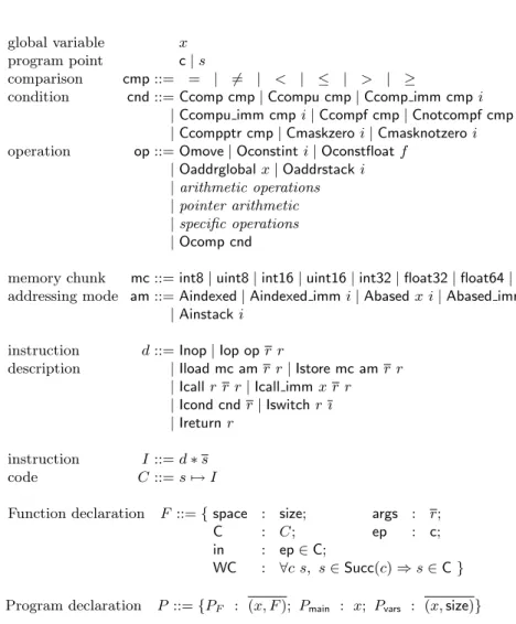
The structure of the RTL language is outlined in figure 2. A full program is composed of a set of function definitions PF represented by a vector of pairs

binding a function name and a function declaration, one of these function names should be declared as the main function Pmain. It also contains a set of global

variable declarations represented by a vector of pairs binding global variable names and their corresponding memory size.

Each function declaration indicates various parameters for this function, like the arguments (args), or the size of the stack memory that is required for local usage (space). Important ingredients are the function code (C) and the entry point (ep). The record also contains “certificates”: the field (in) contains a proof that the entry point is in the code, while the field (WC) contains a proof that the code is a well-connected graph.

(5)

global variable x program point c| s

comparison cmp::= = | 6= | < | ≤ | > | ≥

| Ainstack i instruction d::= Inop | Iop op r r

instruction I ::= d ∗ s code C::= s 7→ I

Function declaration F ::= { space : size; args : r; C : C; ep : c; in : ep ∈ C;

WC : ∀c s, s ∈ Succ(c) ⇒ s ∈ C } Program declaration P ::= {PF : (x, F ); Pmain : x; Pvars : (x, size)}

(6)

The code itself is given as a partial function from a type s of program locations to a type I of instructions. To encode this partial function, we view it as the pair of a total function and a domain predicate. Each instruction combines an instruction description and a vector of potential successors.

Instruction descriptions really specify what each instruction does: memory access, call to other functions, conditional and switch, or return instructions. A “no-operation” instruction is also provided: this instruction is useful to replace discarded instructions without changing the graph shape during optimizations.

Instruction descriptions do not contain the successor of instructions, this in-formation is given at the upper level I by the list of successors. This organization makes it easier to describe some analyses on the code in an abstract way. For most instruction descriptions, exactly one successor is required, except for the Ireturn instruction, which takes no successor, the Icond instruction, which takes two successors and for the Iswitch instruction which takes one successor for each defined label (ı) and one for the default branch.

The syntactic categories of comparison (cmp), condition (cnd) and operation (op) are used to give a precise meaning to the various instructions. Note that the language makes a distinction between several kinds of numbers: integers, un-signed integers, floating point numbers, and pointers. This distinction appears in the existence of several kinds of comparison and arithmetic operations. Op-erations of each kind are distinguished by the suffix u, f, or ptr, or no suffix for plain integers. The arithmetic on pointers makes it possible to compare two pointers, to subtract them (this return a integer), and to add an integer to a pointer. The way pointers are handled in the language is also related to the way memory is handled in the store and load instructions.

Memory access instructions (Iload and Istore) take a memory chunk (mc) parameter that indicates the type of data that is read or written in memory. It also indicates how data is to be completed: when reading an 8-bit integer into a 32-bit register, it is necessary to choose the value of the remaining 24 bits. If the integer is considered unsigned, then the extra bits are all zeros, but if the data is signed, then the most significant bit actually is a sign bit and one may use complement to 2 representation. This way of handling numbers is common to most processors with 32-bit integer registers and 64-bit floating point registers. A second parameter to load and store operations is the addressing mode. This addressing mode always takes two arguments: an address and an offset. The addressing modes given here are especially meaningful for the Power-PC micro-processor.

The language contains two instructions for function calls, Icall imm repre-sents the usual function call where the function name is known at compile-time, whereas Icall represents a function call where the function is given as a loca-tion in a register2_{. This capability is especially useful if we want to use Cminor}

or RTL as an intermediate language for the compilation of functional program-ming languages, where the possibility to manipulate and call function pointers is instrumental.

2

(7)

3.2 Values and memory model

To describe the way memory is handled in our language, we use a model that abstracts away from some of the true details of implementation. This abstraction has two advantages. First, it preserves some freedom of choice in the design of the compiler (especially with respect to stack operations); second it makes the correctness proofs easier. This abstraction also has drawbacks. The main drawback is that some programs that could be compiled without compiling errors and run without run-time error have no meaning according to our semantics.

The first point of view that one may have on memory access is that the memory may be viewed as a gigantic array of cells that all have the same size. Accessing a memory location relies on knowing this location’s address, which can be manipulated just as any other integer. The stack also appears in the memory, and the address of objects on the stack can also be observed by some programs. If this memory model was used, then this would leave no freedom to the compiler designer: the semantics would prescribe detailed information such as the amount of memory that is allocated on the stack for a function call, because this information can be inferred by a cleverly written C program.

In practice, this point of view is too detailed, and the actual value of addresses may change from one run of the same program to another, for instance because the operating system interferes with the way memory is used by each program. The compiler should also be given some freedom in the way compiled programs are to use the stack, for instance in choosing which data is stored in the micro-processor’s registers and which data is stored in the stack.

The abstract memory model that we have designed relies on the following feature: memory is always allocated as “blocks” and every address actually is the pair of a block address and an offset within this block. The fact that we use an offset makes it possible to have limited notions of pointer arithmetic: two ad-dresses within the same block can be compared, their distance can be computed (as an integer), and so on. On the other hand, it makes no sense to compare two addresses coming from two different blocks, this leaves some freedom to the compiler to choose how much memory is used on the stack between two allocated chunks of memory. For extensions of the language, this also makes it possible to have memory management systems that store data around the blocks they allocate.

From the semantic point of view, this approach is enforced by the following features. First, our RTL language has a specific type of memory address for which direct conversion to integer is not possible, but we can add an integer to an address (we enforce the same restriction in our formal semantics of Cminor). Second, any memory access operation that refers to a block of a given size with an offset that is larger than this size has no semantics.

All the syntactic structures used for values and memory are described in Figure 3.

Our memory model relies on block allocation. Some of the blocks are long-lived and stored in the main memory. Other blocks are short long-lived and correspond to local memory used in C functions (the memory allocated on a stack at each

(8)

function call is often referred to as a frame). These blocks are “allocated” when the function is called and “deallocated” when the function returns the control to its caller. It is relevant to make sure that different blocks used for different call instances of functions are really understood as different blocks. To achieve this level of abstraction, we consider that there is an infinity of blocks with different status. Memory is then considered as a mapping from an infinite abstract type of head pointers to a collections of block.

Memory modifications correspond to changing the values associated to these head pointers. In the beginning, most head pointers are mapped to a NotYetAl-located block. When a function is called and a block of memory is alNotYetAl-located for this function, a head pointer is updated and becomes mapped to a vector of elementary memory cells (corresponding to bytes). When the block is released, the head pointer is updated again and becomes mapped to a Freed block. Our semantics description of the language gives no meaning to load and store oper-ation in NotYetAllocated and Freed blocks. In this way, we are able to account for the limited life-span of some memory blocks.

To ensure the clean separation between memory addresses and integer values, we only specify that a memory address requires four bytes for storage3_{. We allow}

writing bytes into a location where an address was previously stored, but this has the side effect of storing an “unknown” value in all the other bytes of the address. We use the symbol ⊥ to denote these unknown values.

Blocks may also contain some code. This feature makes it possible to pass function pointers around and to implement function calls where the function is given by pointer. The level of abstraction is simple to state here: there is no way to know what size a piece of code is taking and only the head pointer of a block containing code may be used in a function call. Of course, reading an integer or an address from a block that contains code simply returns the unknown value ⊥.

head pointer p

memory address a::= (p, n) value v::= n | f | a | ⊥ basic block b::= ⊥ | c | a

block B ::= C | b| Freed | NotYetAllocated memory m::= p 7→ B

load load: m→ mc → a → v loadF : m→ a → F

store store: m→ mc → a → v → m⊥

storeF : m→ mc → a → v → m⊥

Fig. 3.Value and memory

3

(9)

3.3 Semantics

state S::= {Sr: r → v; Sstk: p; Smem: m; Sid: x → v }

condition evalcnd: S→ cnd → r → v

operation evalop: S→ op → r → v

addressing mode evalam: S→ am → r → a⊥

Evaluation of one instruction (selected rules)

(S, (Inop, [s])) 7−→ (S, s)

evalop(S, op, r) = v CheckType(rd, v)

(S, (Iop op r rd,[s])) 7−→ (S[rd:= v], s)

Sid(x) = a loadF(Smem, a) = f InitFun(f, S, r) = S1

(S1, fep) f

7−→ (S2, v) Return(S, S2) = S3 CheckType(rd, v)

(S, (Icall imm x r rd,[s])) 7−→ (S3[rd:= v], s)

Evaluation of several instructions fC(c1) = I (S1, I) 7−→ (S2, c2) (S2, c2) f 7−→ (S3, v) (S1, c1) f 7−→ (S3, v) fC(c) = (Ireturn r, ∅) (S, c)7−→ (S, S.(r))f Evaluation of a program

InitProg(p) = S pF(pmain) = f InitFun(f, S, ∅) = S1

(S1, fep) f

7−→ (S2, v) Return(S, S2) = S3

p7−→ (SP 3, v)

Fig. 4.Semantics of RTL

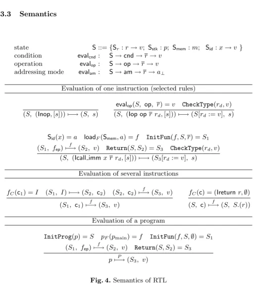
Figure 4 outlines the semantics of RTL. Some parts are given by inductively defined relations, while other parts are given by functions. Important data for these relations and functions is collected in a structure named a state. The component named Sr is a function that gives the value of all registers. The

component Sstk indicates the current position of the stack top; this position

can be used as a head-pointer for access in the memory allocated for the current function call instance. The component Smemcontains the description of the whole

memory state. The component Sidindicates the values associated to all the global

variables (identifiers).

The semantics of individual instructions is described as an inductive relation using a judgment of the form (S, I) 7−→ (S′_{, s), where S is the input state,}

I is the instruction to execute, S′ _{is the result state, and s is the location of}

(10)

judgment. Each rule contains a few consistency checks: for instance, instructions expecting a single successor should not receive several potential successors, the registers providing the input for an arithmetic operation should contain values of the right type, and the register for the output value should also have the right type.

To describe the execution of several instructions, we use a judgment of the form (S, c)7−→ (Sf ′_{, v), where f is a function, c is the location of an instruction in}

the code graph of f , S′_{is the result state when the function execution terminates}

and v is the return value. So while the judgment (S, I) 7−→ (S′_{, s) is given in a}

style close to small step operational semantics, the judgment (S, c)7−→ (Sf ′_{, v)}

describes a complete execution as we are accustomed to see in big step operational semantics or natural semantics. The two styles actually intertwine in the rule that describes the execution of the Icall imm instruction: to describe the behavior of the single Icall imm instruction, this rule requires that the code of the callee is executed completely to its end.

The rule for the Icall imm instruction first states that the function code must be fetched from memory, then that some initialization must be performed on the state. This initialization consists of allocating a new memory block for the data that is local to the function and moving the Sstk field. Then, verifications

must be performed: the registers that are supposed to contain the inputs to the called function must contain data of the right type. The registers that are used internally to receive the input arguments must be initialized. Then the function code is simply executed from its entry point, until it reaches a Ireturn statement, which marks the end of the function execution. An auxiliary function, called Returnthen modifies the state again, restoring the Sstk field to its initial value

and freeing the memory block that had been allocated.

Evaluating a program is straightforward. Some initialization is required for the global variables and the main function of the program is executed to its end. When proving the correctness of optimizations, we intuitively want to prove that an optimized function performs the same computations as the initial func-tion. A naive approach would be to express that the resulting state after exe-cuting the optimized function is the same as the resulting state after exeexe-cuting the initial function. However, this approach is too naive, because optimization forces the state to be different: since the function code is part of the program’s memory, the optimized program necessarily executes from an initial state that is different and terminates in a state that is different. Our correctness statement must therefore abstract away from the details concerning the code stored in the memory.

4 A generic proof for the optimizations

In the sequel, we consider two optimization phases from RTL to RTL, the first one is constant propagation (CP) and the second is common subexpression elimina-tion (CSE). Both are done procedure by procedure and follow the same scheme.

(11)

The first step is a data-flow analysis of the procedures. The result of this analysis is a map that associates to each program point the information that is “valid” before its execution. By “valid information” we mean that any execution would reach this program point in a state that is compatible with the value predicted by the analysis.

The second step is the transformation of the code. This transformation is done instruction by instruction and only requires the result of the analysis for one instruction to know how to transform it. Naturally, the power of the trans-formation depends directly on the analysis.

We wrote a generic program and its proof to automatically build the analyses, the transformations, and their proofs.

4.1 Analysis specification

A data-flow analysis is given by a set D (the domain of the analysis) representing abstractions of states and an analysis function AF that takes as input a function

declaration and returns a map from program points to D. These two parameters represent the computation part of the analysis. For CP and CSE the domain is a mapping from registers to abstract values, e.g. a concrete value or “unknown” for CP, or a symbolic expression for CSE.

An analysis is correct when it satisfies some extra properties. In particular, we need an analysis property AP that describes when a concrete state in S is

compatible with an abstract state in D. The result of the analysis should have the property that every reachable instruction can only be reached in a state that is compatible with the abstract state that is predicted by the analysis.

The first part of the correctness statement expresses that every state should be compatible with the abstract point that is computed for the entry point; this statement is called Aentry.

The second part of the correctness statement expresses that every computa-tion state should map a state compatible with the abstract state for an instruc-tion to states that are compatible with the abstract states of all the successor; this statement is called Acorrect.

All the components of a valid analysis are gathered in a module type for Coq’s module system.

Module Type ANALYSIS. Parameter D : Set. Parameter AF : F → Map.T D. Parameter AP : D → S → Prop. Parameter Aentry : ∀f S, AP(AF(fep), S). Parameter Acorrect : ∀f c1 c2 S1 S2, c1∈ fC⇒ (S1, fC(c1)) 7−→ (S2, c2) ⇒ AP(AF(c1), S1) ⇒ AP(AF(c2), S2). End.

Correct analyses can be obtained in a variety of ways, but we rely on a generic implementation of Kildall’s algorithm [2]: the standard solver for

(12)

data-flow equations using a work list. To compute an analysis, Kildall’s algorithm observes each instruction separately. Given a program point c, it computes the value of the analysis for the instruction c using a function Ai. Then it update

the abstract state of every successor of c with an upper bound of itself and the value of Aiat c. The function Ai is the analysis of an instruction, it takes what

is known before the instruction as argument and returns what is known after it. The termination of this algorithm is ensured because the code graph for a function is always finite and the domain of the analysis is a well-founded semi-lattice : a set D with a strict partial order >D, a decidable equality, a function

that returns an upper bound of every pair of elements, and the extra property that the strict partial order is well-founded.

We don’t give more details about Kildall’s algorithm, for lack of place, but in our formal development, it is defined using Coq’s module system as a functor (a parameterized module) taking as arguments the well-founded semi-lattice, the analysis function, and a few correctness properties. This functor is in turn used to define a generic functor that automatically builds new analyses. This functor takes as argument modules that satisfy the following signature:

Module Type ANALYSIS ENTRIES. Declare Module D : SEMILATTICE. Parameter Ai : F → c → D.T → D.T .

Parameter AP : D.T → S → Prop.

Parameter topP : ∀S, AP(D.top, S).

Parameter Acorrect : ∀f c, c ∈ fC⇒

∀c′ _{S S}′_, _{(S, f}

C(c)) 7−→ (S′, c′) ⇒ ∀d, AP(d, S) ⇒ AP(Ai(d, c), S′).

Parameter A≥D : ∀d1 d2, d2≥Dd1⇒ ∀S, AP(d1, S) ⇒ AP(d2, S).

End.

Module Make Analysis (AE : ANALYSIS ENTRIES) <: ANALYSIS.

First, the semi-lattice’s top element should be compatible with any state (topP). At the entry point we make the assumption that nothing is known,

hence the initial abstract state of the analysis is top. This property ensures that any initial state will satisfy the analysis property at the entry point. Second, the parameter Acorrect ensures that each time the Kildall algorithm analyzes

an instruction the result will be compatible with the states occurring in the concrete execution. Then, the last property A≥_Dexpresses that the order relation

on abstract states should be compatible with the subset ordering on S. This ensures that each time Kildall’s algorithm computes a new upper bound, the result remains compatible.

4.2 Program transformations

The second part of an optimization is a transformation function that uses the results of the analysis to change the code, instruction per instruction. Here again, there is a generic structure for CP and CSE. First, a transformation is given by

(13)

two functions TFand TPto transform function declarations and whole programs,

respectively. The correctness of this transformation is expressed by saying that executing a program to completion should return the same result and equivalent states, whether one executes the original program or the optimized one (Tcorrect).

Two states are equivalent when all locations in the memory have the same value, except that unoptimized code is replaced with optimized code, using a generic replacement map called Tstate.

Module Type TRANSFER. Parameter TF : F → F . Parameter TP : P → P . Parameter Tcorrect: ∀p S v, p P 7−→ (S, v) ⇒ TP(p) P 7−→ (Tstate(TF, S), v). End.

Here again, correct transformations can be obtained in a variety of ways, but we rely on a generic implementation that takes a correct instruction-wise transformation as a parameter.

We actually describe instruction-wise transformations that rely on an analysis A. The transformation itself is given by a function Ti, which takes as input an

instruction and the abstract state capturing what the compiler knows about the state before executing this instruction, and returns a new instruction. The correctness of this transformation is then expressed by a few extra conditions. First, the successors of the new instruction should be a subset of the original successors (Tedges). Second the execution of the transformed instruction in a state

that is compatible with the abstract state obtained from the analysis should lead to the same new state and the new location in the code (Tcorrect). Third, a

return instruction should be left unchanged (Treturn). Fourth, the compatibility

of a state with respect to an abstract state should not depend on the actual code functions that is stored in memory. All these aspects of an instruction-wise transformation are gathered in a module type TRANSFER ENTRIES.

Correct instruction-wise transformations never remove any instruction from the code graph. On the other hand, they may remove edges, if the analysis makes it possible to infer that these edges are never traversed during execution. This treatment also means that dead code is optimized at the same time as useful code. The actual removal of dead code is not part of these optimizations, it is just a side effect of the later translation from the LTL language to the Linear language.

Module Type TRANSFER ENTRIES. Declare Module A : ANALYSIS. Parameter Ti : A.D → I → I.

Parameter Tedges: ∀d i s, s ∈ Succ Ti(d, i) ⇒ s ∈ Succ i.

Parameter Tcorrect : ∀i s S S′ d, AP(d, S) ⇒

(S, i) 7−→ (S′_{, s) ⇒ (S, T}

i(d, i)) 7−→ (S′, s).

Parameter Treturn: ∀d r s, Ti(d, (Ireturn r, s)) = (Ireturn r, s).

Parameter Amem : ∀(g : F → F ) d S, AP(d, S) ⇒ AP(d, Tstate(g, S)).

(14)

Transformations are thus obtained through an application of a functor that takes modules of type TRANSFER ENTRIES as input and returns modules of type TRANSFER. Some parts of the correctness proofs are done once and for all in this functor, but other parts are specific and done when establishing the facts Tedges, Tcorrect, Treturn, and Amem, which represent a big part of the proof (in

number of lines) but are usually easy.

5 Instantiation

In this section we describe how we instantiate our functors to obtain the CP and CSE optimizations. The term optimization is a misnomer because there is no guarantee that the result code is the best possible. It is only the best that we can obtain using the information gathered by the analysis.

5.1 Constant propagation

The role of constant propagation is to replace some operations by a more efficient version: for example, by a “load constant” instruction when the result of the operation is known at compile time, or by an immediate operation when only one argument is known.

To use our predefined functor for analysis and transformation, the most diffi-cult part is to define the semi-lattice corresponding to the domain of the analysis. Here, the goal of the analysis is to collect the known values associated to each register.

The domain of the analysis is the set of maps that associate to each register a numerical value when it is known. The set of maps from A to B is a semi-lattice if B itself is a semi-lattice and if A is a finite set. Therefore, we need to limit the number of registers. This is done using a dependent type: a register is a pair of a number (its identifier) and a proof that this identifier is less than a parameter map limit.

We define the semi-lattice corresponding to the codomain of the maps as the flat semi-lattice build upon the type of values that we can associate to registers at compile time :

v::= n | f | (x, n)

that is, an integer, a float or the address of a known global variable plus an offset. Such a construction is possible since the equality on the type v is decidable.

The analysis of an instruction consists in evaluating its result value and updating the register where the result is stored with this value. Naturally, this evaluation is only possible if all the arguments of the instruction have known values. Otherwise, the result register is set to top. The correctness criterion for this analysis is that if it claims that a register has a known value at some point, the actual value of the register at this point in every execution is equal to the claimed value.

Then, the transformation of an instruction first tries to evaluate the instruc-tion and replaces the instrucinstruc-tion by an instrucinstruc-tion that directly stores the result

(15)

in a register, when this is possible. For example, if r1 = 1 and r2 = 3 the

instruction Iop Oadd r1 r2 rd will be replaced by Iop (Oconstint 4) rd.

If only some of the arguments are known, then the transformation tries to replace the instruction by a more efficient one. For example, if r2 = n,

then Iop Omul r1 r2 rd will be replaced by Iop (Oconstint 0) rd if n = 0, by

Iop Omove r1 rd if n = 1, by a left shift over r1if n a is a power of two, or by a

immediate multiplication Iop (Omul imm n) r1rd otherwise.

Memory access is also optimized using a based addressing mode if the address is known at compile time. Finally, conditional branches are replaced by an Inop instruction, actually implementing an unconditional branch to the appropriate successor, if the result of the test is statically evaluable.

5.2 Common subexpression elimination

A program will frequently include multiple computations of equivalent expres-sions, e.g. array address calculations. The goal of common subexpression elim-ination is to factor out these redundant computations. An occurrence of an expression E is called a common subexpression if E was previously calculated and the values associated with the register that appear in E have not changed since the previous computation. In this case the compiler can replace the second occurrence of E by an access to the register containing the result of the first occurrence of E, thus saving the cost of recomputing E.

For example the sequence :

r3= r1+ r2; r4= r1; r5= r4+ r2

will be replaced by :

r3= r1+ r2; r4= r1; r5= r3

Here the result of the analysis of an instruction is a map that associates to each register a symbolic expression corresponding to the operation that is stored in it. More precisely, the values associated to registers are a pair of a symbolic expression (the expression whose result is contained in the register) and a set of registers which contain the same value. The latter set is useful to keep track of multiple registers containing the result of the same computation, as often occurs following Imove instructions, and determine equivalence of symbolic expressions up to Imove instructions. For instance, in the code fragment above, it is known that the symbolic expressions r1+ r2and r4+ r2 are equivalent because r1 and

r4 contain the same value. Futhermore, we want to keep track that r3 and r5

contain the same value, even after a modification of r2 that will invalidate the

expression associated to both registers.

A concrete register set matches the result of the analysis at a given program point if the actual values of the registers satisfy the equalities between registers stated in the abstract values. The mappings of registers to symbolic expressions can be equipped with a well-founded semi-lattice structure, with the least upper

(16)

bound operation corresponding roughly to the intersection of constraints. This semi-lattice construction is complex and we omit it here due to lack of space.

The analysis of an instruction that computes E and stores its result in a register rd first erases all references to rd in the map. If the register rd is not

used as arguments of the instruction then the analysis tries to find a register containing an expression equivalent to E. In this case, the analysis updates the value associated to rd with the expression and the set of registers that contain

the equivalent expression. It also adds the fact that registers in the set are all equal to rd. In all other cases, the value associated with rdis set to the expression

E and an empty set of equal registers.

The transformation of an instruction rd= E is refreshingly simple: it becomes

rd = r (a Imove instruction) if there exists a register r that contains the value

of E, and is left unchanged otherwise. The Imove instructions thus introduced can disappear later during register allocation, if the register allocator manages to assign the same hardware register or stack location to both r and rd.

6 Related work and conclusions

In parallel with our work, several other teams developed machine-checked proofs of data-flow analyses and transformations. For instance, Cachera et al [1] develop in Coq a general framework for lattices and data-flow equations over these lat-tices. Their framework is more general than ours, but they do not consider pro-gram transformations. Proofs of Kildall’s work-list algorithm can also be found in machine-checked formalizations of Java byte-code verification such as [3].

Lerner et al [4] propose Rhodium, a domain-specific language to express data-flow analyses and transformations exploiting the results of these analyses. Rhodium generates an implementation of both the analysis and the transforma-tion and proof obligatransforma-tions that, once checked, imply the semantic correctness of the transformation. Rhodium specifications are definitely more concise than in-stantiations of our generic framework. However, the generated proof obligations do not appear significantly simpler than the proofs we have to provide for our functor applications. Moreover, the Rhodium tools must be trusted to generate correct implementations and sufficient proof obligations, while we obtain these guarantees by doing everything directly in Coq.

In summary, by exploiting the Coq module system, we have been able to factor out a significant part of specifications and correctness proofs for forward data-flow analyses and optimizations that exploit the results of these analyses. While the application of this framework to constant propagation is fairly stan-dard, we believe we are the first to develop a mechanically verified proof for common subexpression elimination using the “Herbrand universe” approach.

While this is not described in this paper, backward data-flow analyses is handled by a simple extension of our framework (basically, just reversing the control flow graph before using the forward analysis framework). We used this to prove correct liveness analysis as used in our register allocation phase.

(17)

A limitation of our approach, also found in Rhodium, is that we prove the correctness of transformations using simulation arguments that apply only when every instruction of the source code is mapped to zero, one or several instructions of the transformed code, and the states “before” and “after” the source instruc-tion must match the states “before” and “after” the sequence of transformed instructions. This is not sufficient to prove some optimizations such as code motion, lifting of loop-invariant computations, or instruction scheduling, where computations occur in a different order in the source and transformed code. Be-cause of this limitation, we envision to perform some optimizations such as loop optimizations not on the unstructured RTL intermediate code, but on the struc-tured Cminor source code, whose big-step semantics makes it easier to reorder computations without worrying about intermediate computational states that do not match.

References

1. D. Cachera, T. Jensen, D. Pichardie, and V. Rusu. Extracting a data flow analyser in constructive logic. In 13th European Symposium on Programming (ESOP’04), volume 2986 of Lecture Notes in Computer Science, pages 385–400. Springer-Verlag, 2004.

2. G. A. Kildall. A unified approach to global program optimization. In 1st symposium on Principles of Programming Languages, pages 194–206. ACM Press, 1973. 3. G. Klein and T. Nipkow. Verified bytecode verifiers. Theoretical Computer Science,

298(3):583–626, 2002.

4. S. Lerner, T. Millstein, E. Rice, and C. Chambers. Automated soundness proofs for dataflow analyses and transformations via local rules. In 32nd symposium on Principles of Programming Languages, pages 364–377. ACM Press, 2005.

5. G. Morrisett, D. Walker, K. Crary, and N. Glew. From system F to typed assembly language. ACM Transactions on Programming Languages and Systems, 21(3):528– 569, 1999.

6. G. C. Necula. Proof-carrying code. In 24th symposium Principles of Programming Languages, pages 106–119. ACM Press, 1997.

7. A. Pnueli, M. Siegel, and E. Singerman. Translation validation. In Tools and Algorithms for Construction and Analysis of Systems, TACAS ’98, volume 1384 of Lecture Notes in Computer Science, pages 151–166. Springer, 1998.