Coherence characterization with a superconducting flux qubit through NMR approaches

Coherence Characterization with a

Superconducting Flux Qubit through NMR

Approaches

by

Fei Yan

Submitted to the Department of Nuclear Science and Engineering

in partial fulfillment of the requirements for the degree of

Doctor of Philosophy in Nuclear Science and Engineering

^

at the

MASSACHUSETTS INSTITUTE OF TECHNOLOGY

June 2013

@

Massachusetts Institute of Technology 2013.

ARCHNES

*S^CHUET IN81?'S

OFTECHNOLOj0GS-yT-JUL 16 2013

LIBRARIES

All rights reserved.

Author...

Department of Nuclear Science and Engineering

May 8, 2013

Certified by...

---~

-- fraid G. Cory

Professor of Chemistry, University of Waterloo

a 1

_ hesis, Supervisor

C ertified by ...

_...

Terry P. Orlando

Professor of Electrical Engineering and Computer Science

Thesis Reader

C ertified by ...

...

Paola Cappellaro

Assistant Professor of Nuclear Science and Engineering

--Thesis Reader

A ccepted by ... ...

...

KMu

d S. Kazimi

TEPCO Professor of Nuclear Engineering

Coherence Characterization with a Superconducting Flux

Qubit through NMR Approaches

by

Fei Yan

Submitted to the Department of Nuclear Science and Engineering on May 8, 2013, in partial fulfillment of the

requirements for the degree of Doctor of Philosophy

Abstract

This thesis discusses a series of experimental studies that investigate the coher-ence properties of a superconducting persistent-current or flux qubit, a promising candidate for developing a scalable quantum processor. A collection of coherence-characterization experiments and techniques that originate from the field of nuclear magnetic resonance (NMR) are implemented. In particular, one type of dynamical-decoupling techniques that uses refocusing pulses to recover coherence is successfully realized for the first time. This technique is further utilized as a noise spectrum ana-lyzer in the megahertz range, by which a 1/f-type dependence is observed for the flux noise. Then, a novel method of performing low-frequency noise spectroscopy is devel-oped and successfully implemented. New techniques used in the readout scheme and data processing result in an improved spectral range and signal visibility over con-ventional methods. The observed power law dependence below kilohertz agrees with separate measurements at higher frequencies. Also, the noise is found to be temper-ature independent. Finally, a robust noise spectroscopy method is presented, where the spin-locking technique is employed to extract noise information by measuring the driven-evolution longitudinal relaxation. This technique shows improved accuracy over other methods, due to its insensitivity to low-frequency noise. Spectral signa-tures of coherent fluctuators are resolved, and further confirmed in a time-domain spin-echo experiment.

Thesis Supervisor: David G. Cory

Title: Professor of Chemistry, University of Waterloo

Thesis Reader: Terry P. Orlando

Title: Professor of Electrical Engineering and Computer Science

Thesis Reader: Paola Cappellaro

i -- &L. # 1t

h

Acknowledgments

Now as I am writing this last part of my own thesis on my 27th birthday, many faces and things are brought to mind. This unique journey of pursuing a PhD is a mixture of various feelings, and I could not have made it through without the guidance and support from many people.

First, I want to thank my mother Rongxia and father Yong for their generous love and support throughout my life. Making them proud has been an important motivation behind everything I have accomplished in my life. Being their only child, I often feel guilty that I spent too less time with my family during these five years. To them is dedicated this thesis.

I left my hometown, Nanjing, and started my journey in Cambridge under the supervision of Prof. David Cory, to whom I am exceptionally grateful for bringing me to MIT, for introducing me to the fascinating quantum world, for offering me precious research opportunities, for guiding my academic life, for helping me explore my future. Since David moved to Waterloo in 2010, we have had much less overlap. However, it was in my senior years that I started to realize that many things he said about research in the very early days of my PhD life are true! To me, he seems to know everything but touches only a little bit, and lets myself explore. I would really die for understanding his provident ideas and visions. In many senses, he is a myth to me, which makes me respect him even more.

I would also like to thank all the Cory group members - past and present - with whom I have worked, in particular Clarice Aiello, Sarah Sheldon, Kevin Krsulich and Leslie Dewan for all the classes attended together; Troy Borneman, Jonathan Hodges and Kai Iamsumang, with whom I shared the office and had fruitful discussions; Paola Cappellaro for being my academic advisor and sharing ideas in research; and Chandrasekhar Ramanathan for teaching me quantum mechanics. Many thanks also to all the other group members: Mohamed Abutaleb, Cecilia Lopez, Dmitry Pushin, Jamie Yang, Rui Xian. I am also thankful to Jennifer Choy, a former group member, for a great time shared during a conference.

Since I entered MIT, I have also been closely associated with Prof. Terry Or-lando's superconducting circuits and quantum computation group. In fact, due to the collaboration between Terry and David, I did most of my research in the Orlando lab. I really appreciate him for the great research opportunities and generous support throughout my PhD life. Terry is the kind of person who is likely to accept whatever the fate is and be happy about it. Although he intervenes with lab issues less often in these years, whenever you need help, he is always there and sets up everything in a nice manner.

Will Oliver is a senior research scientist in the Orlando group. He is effectively the manager of this lab, motivating and guiding everyone. To me, he is a real mentor, who teaches me a lot about the field of superconducting qubits, helps me explore my academic life, pushes me to challenge myself, influences me with his character. Will is truely a wise man. He is knowledgeable, but never brags about. He is confident, but never ignores anyone who needs his attention. He appreciates others' nice work, but never looks down on ourselves. He is ambitious, but always does things with patience. He is a thinker, but always communicates with everyone effectively. He is a busy scientist, but always gets his husband and father job done. All of these make me feel honored to be working with him.

Jonas Bylander and Simon Gustavsson, two Swedish postdocs in the Orlando group, are the guys I have the most overlap with during my PhD life. Jonas is the very first person who teaches me how to be an experimentalist. I learned a lot from him on how to run the dilution fridge, how to properly use electronics and how to present results. I am grateful for his trust on me to run my own experiments in the million-dollar lab. He is a kind and humorous person, who also helps me a lot in life issues. On the other hand, Simon contributes the most to my final PhD works. Since

I started to do my own experiments in my third year, he has become the most helpful

person in the lab. Whenever I encounter some problems that I cannot figure out, he is always willing to help me and teach me with patience. In addition, he is the most efficient guy I have ever seen, in terms of the speed of finishing work, in terms of the number of quality papers in a year and in terms of enjoying life on mountains every

weekend. I have a high regard for him, and wish myself to be like him.

I also have the opportunity to work closely with other members -past and present

- in this group, which includes Xiaoyue Jin, a postdoc with whom I can enjoy speaking Chinese in the lab; Philip Krantz, a visiting student with whom I enjoy sailing with; and Olger Zwier, another visiting student with whom I enjoy being a teacher at some times. Though never met, I would also thank David Berns, a former student in this group, for all the books and materials he left in his office which I took over later. That is a real fortune for me.

All the friends that I have met here have been invaluable to make my experience

here so enriching. I thank Yue Fan and Weishan Chiang for being my buddies entering the same department in the same year, taking classes and working on problem sets together and rumbling about graduate student life. I thank Rong Zhu and Zhizhong Li for being the longtime teammates on the basketball court. I thank Jing Yuan for being my four-year roommate. I thank Xiaoman Duan, He Wei, Benyue Liu, Mo Jiang, Kailiang Chen, Wenjing Fang, Xi Yang, Bing Wu, Yingxue Wang, Liyao Wang, Tianqi Li, Hai Wang, Zhihao Jiang, Yang Liu, Liang Pang, Jing Gao, Da Lu, Lin Li and all the friends in Chinese Student and Scholar Association for coloring my lonely PhD journey.

Last but not least, I want to thank my beloved old friends, in particular SW, MR,

Contents

1 Introduction 21

1.1 Quantum Computer and Decoherence . . . . 21

1.2 Outline of this Thesis . . . . 24

2 System Dynamics with NMR-like Manipulation 27 2.1 Introduction . . . . 27

2.2 Bloch Sphere Representation . . . . 27

2.3 Laboratory Frame and Quantization . . . . 32

2.4 Radiofrequency Pulse . . . . 35

2.4.1 Rotating Frame . . . . 38

2.4.2 Single Pulse . . . . 41

2.4.3 Multiple Pulses . . . . 43

2.5 Free Evolution and Related Experiments . . . . 44

2.5.1 Free Evolution and Its Decoherence . . . . 44

2.5.2 Inversion Recovery . . . . 51

2.5.3 Free Induction . . . . 53

2.5.4 Spin Echo and Carr-Purcell Sequence . . . . 58

2.6 Driven Evolution and Related Experiments . . . . 62

2.6.1 Driven Evolution and Its Decoherence . . . . 63

2.6.2 Spin Locking . . . . 75

2.6.3 Rabi Precession . . . . 77

2.6.4 Rotary Echo . . . . 80

3 A Superconducting Qubit: The Persistent-Current Qubit 3.1 Introduction . . . .

3.2 The Persistent-Current Qubit . . . .

3.2.1 Josephson Junction . . . .

3.2.2 The Persistent-Current Qubit . . . .

3.2.3 Tight-Binding Model and Two-Level Approximation 3.2.4 The SQUID Detector . . . .

3.3 Device Description and Measurement Setup . . . .

4 Basic Coherence Characterization Methods

4.1 Introduction . . . . 4.2 Qubit Spectrum . . . . 4.3 Free-Evolution Coherence Characterization . . . .

4.3.1 Inversion Recovery and High-Frequency Noise Spectroscopy 4.3.2 Free Induction Decay and Quasistatic Noise . . . . 4.3.3 Spin Echo and Carr-Purcell-Meiboom-Gill Spectroscopy . . .

4.3.4 Temperature Dependence . . . . 117

4.4 Driven-Evolution Coherence Characterization . . . . 4.4.1 The Rabi Spectroscopy . . . . 4.4.2 Rotary Echo . . . . 4.5 Summary . . . . 5 Repeated Fixed-Time Free Induction and Low-Frequency troscopy 5.1 Introduction . . . . 5.2 Low-Frequency Noise Spectroscopy . . . . 5.3 The Repeated Fixed-Spacing Free-Induction Experiment 5.3.1 Method and Analysis . . . . 5.3.2 Temperature Results . . . . 5.3.3 A -E Correlation . . . . 5.4 Sum m ary . . . . Noise Spec-131 . . . . 131 . . . . 132 . . . . 134 . . . . 138 . . . . 145 . . . . 148 . . . . 149 85 . . . . . 85 . . . . . 86 . . . . . 88 . . . . . 91 . . . . . 94 . . . . . 97 . . . . . 100 107 107 107 108 108 110 113 126 126 128 129

6 A Better Noise Spectroscopy Method: The Tp Experiment 151

6.1 Introduction ... ... 151

6.2 The Spin-Locking Dynamics . . . . 153

6.2.1 The Original Sequence and System Dynamics . . . . 154

6.2.2 Comparison with other Methods . . . . 155

6.3 Robust Sequences . . . . 158

6.3.1 5-Pulse Sequence and Cancellation of Dephasing Effect . . . . 158

6.3.2 Twin Sequence and Recovery from Ultra-Low-Frequency Signal D istortion . . . . 159

6.4 R esults . . . . 161

6.5 Time-Domain Confirmation . . . . 165

6.6 Temperature Dependence . . . . 169

6.7 Sum m ary . . . . 170

7 Summary and Future Work 173 7.1 Sum m ary . . . . 173

7.2 Future W ork . . . . 175

7.2.1 In-Plane dc Field . . . . 175

7.2.2 The Modified Two-Dimensional Exchange Experiment . . . . 175

7.2.3 The p-Qubit . . . . 175

A Quantum Noise 177 B Definition 179 B.1 Confusion about Correlator . . . . 180

B.2 Confusion about Fourier Transform . . . . 180

B.3 Confusion about Frequency Representation . . . . 181 C Correction Factor from Quasistatic Noise 183

List of Figures

2-1 Bloch picture of the quantum Larmor precession. . . . .

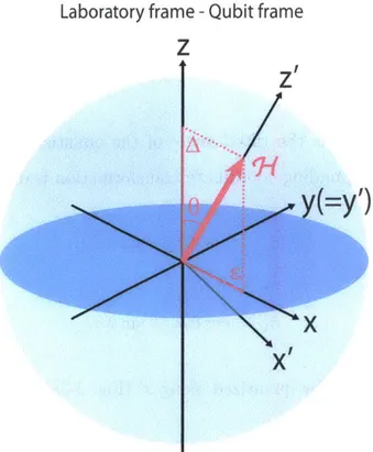
2-2 Bloch representation of a static Hamiltonian and transformation be-tween the laboratory frame and the qubit frame. . . . .

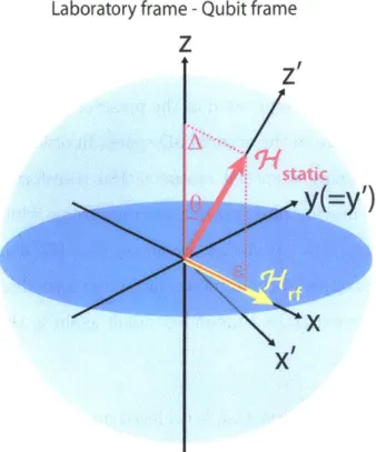
2-3 Quantization and the "south pole ++ ground state" convention... 2-4 Bloch representation of a driven Hamiltonian. . . . .

2-5 Transformation between the qubit frame and the rotating frame. . . .

2-6 Bloch representation of the driven Hamiltonian in the rotating frame. 2-7 2-8 2-9 2-10 2-11 2-12 2-13 2-14 2-15 2-16 2-17 2-18 2-19 2-20 2-21 2-22 Resonant drive. . . . . Single pulse and Rabi precession. . . . . Free-evolution dynamics in the qubit frame. . . . . Inversion-recovery pulse sequence and dynamics. . . . . . Free-induction pulse sequence and dynamics. . . . . Examples of filter functions. . . . . Spin-echo pulse sequence and dynamics. . . . . CP and CPMG pulse sequence. . . . .

Driven-evolution dynamics in the rotating frame... Illustration of noise selectivity. . . . . Sketch of the free-induction and Rabi filter function. . .

Analogy between free- and driven-evolution experiments. Spin-locking pulse sequence and dynamics. . . . . Rabi pulse sequence and dynamics. . . . . Rotary-echo pulse sequence and dynamics. . . . . Generalized rotary-echo pulse sequence. . . . .

29 33 35 37 39 40 . . . . 41 . . . . 42 . . . . 48 . . . . 52 . . . . 55 . . . . 58 . . . . 60 . . . . 62 . . . . 66 . . . . 69 . . . . 70 . . . . 74 . . . . 76 . . . . 78 . . . . 81 . . . . 81

3-1 Schematic diagram of an LC circuit. . . . .

3-2 Energy diagram of a quantum harmonic oscillator. . . . . 3-3 Josephson junction. . . . .

3-4 Schematic diagram of the equivalent circuit of a Josephson junction.

3-5 Energy diagram of a nonlinear LC circuit. . . . . 3-6 Schematic diagram of the flux qubi

3-7 2D potential landscape and the do 3-8 Energy diagram of the flux qubit.

3-9 3-10 3-11 3-12 3-13 3-14

DC SQUID and rapid readout. . .

Device and measurement circuitry. Simulated energy structure. .

Readout-pulse calibration... Picture of the microwave package. Picture of the dilution refrigerator

4-1 Saturated frequency spectroscopy. 4-2 Example trace of measured inversio 4-3 4-4 4-5 4-6 4-7 4-8 4-9 4-10 4-11 4-12 4-13 4-14 4-15

Flux-bias dependence of measured Example trace of measured free ind Example trace of measured spin ec Flux-bias and pulse-number depen Noise spectroscopy by the CPMG,

t . . . . 9 3

ible-well lattice cell. . . . . 94

. . . . 9 6 . . . . 9 9 . . . . 10 1 . . . . 10 2 . . . . 10 3 . . . . 10 4 insert. . . . . 105 ... 108 n recovery. . . . 109

relaxation and dephasing. . . . 111

uction. . . . 112

ho. . . . 114

lence of measured CPMG. . . . 115

Rabi and T method. . . . 117 Example trace of measured inversion recovery with improved average. Example trace of measured free induction with improved average. Example trace of measured sin echo with improved average... Temperature dependence of T measured at E = 0. . . . .

Temperature dependence of T1 measured at E = 640 MHz. . . . .

Temperature dependence of ( and r measured at E = 0. . . . .

Temperature dependence of and measured at e = 640 MHz. Temperature dependence of ,(E and F(SE measured at E = 0. .

118 119 119 120 120 121 121 122 87 88 89 90 91

4-16 4-17 4-18 4-19 4-20 4-21 4-22

Temperature dependence of r(E) and FrSE measured at 6 = 640 MHz.

Temperature dependence of r1 with fit to the quasipartical model. Quadratic temperature dependence ofr ( )2. . . . .

White noise measured by free induction, spin echo and T,. . . . . Example trace of measured Rabi. . . . . Noise extraction from Rabi decay. . . . . Comparison between measured Rabi and rotary-echo decay . . . .

5-1 Measured dependence of switching probability on detuning. . . . . 5-2 Sketch of the PSD, indicating the frequency intervals resolved by the ensemble-averaging and single-shot schemes. . . . .

5-3 Example of SQUID-switching events measured on an oscilloscope. . . 5-4 Measured noise spectra at different temperatures.

122 123 124 125 126 127 129 136 137 139 . . . . 146

Temperature dependence of integrated noise. . . . . Noise correlation. . . . . Illustration of the rotating-frame relaxation. . . . . SL-3 pulse sequence and dynamics. . . . . SL-5a pulse sequence and removal of the dephasing effect.. SL-5b pulse sequence and removal of the detuning effect. Measured F1 and ]1, at e = 0. . . . . Extracted A-noise PSD with error bars. . . . . Measured IF and 1Pi at E

>

0. . . . . Extracted E-noise PSD with error bars. . . . . Noise spectroscopy by the T, method. . . . . 147 149 . . . . . 154 . . . . . 156 . . . . . 159 . . . . . 161 . . . . . 163 . . . . . 164 . . . . . 165 . . . . . 166 . . . . . 167

Temporal signature of the spectral "bump" during spin-echo decay. . Temperature dependence of A-noise PSD. . . . . Temperature dependence of A-noise PSD over a wider frequency range. 168 169 170 7-1 Noise spectroscopy by various methods. . . . . 174

C-1 Sketch of the PSD with relevant frequency intervals. . . . . 185 5-5 5-6 6-1 6-2 6-3 6-4 6-5 6-6 6-7 6-8 6-9 6-10 6-11 6-12

List of Tables

2.1 Comparison of decohering properties during free evolution and driven evolution. . . . . 83

Chapter 1

Introduction

1.1

Quantum Computer and Decoherence

In the past decade, the field of quantum information and quantum computation [1] has developed rapidly and become a hotspot of the physical science. Richard Feynman first suggested the possibly better efficiency in simulating a quantum system by a quantum computer, made of quantum bits (qubits), than the classical computer, made of classical bits [2]. Such quantum computer harnesses the power of quantum superpositions and entanglement to speed up computation. The concept did not draw much attention though until Peter Shor introduced his algorithm [3] and quantum error correction [4].

The power of this super fast computing comes from the natural parallelism created

by quantum superposition. Unlike classical bits, whose instantaneous value must be

either 0 or 1, a qubit can be the superposition of both eigenstates, 10) and ji). In quantum mechanics [5], the system's state is described by the wave function |IT). For N qubits, the wave function of the whole system is generally a linear combination of all the possible ₂N eigenstates,

e T) = C1000 ... 000) + c2l000 -u-b- 001) + orm+

proba-bility of observing the qubit at the jth state in measurement. The magic of quantum mechanics is that a quantum transformation of this system,

I

) -+ U

l

T), operates on all the 2N states simultaneously. Unlike classical parallelism, where multiple circuits

are built to execute a same operation (which would require N x ₂N identical bits),

quantum parallelism only requires N qubits. However, measurement will cause the system to collapse to only one of the states with certain probability. To make the quantum parallelism useful, this requires the ability to extract information from the superposition state, and this is called a quantum algorithm. It has been shown that

a quantum computer can be substantially more efficient than its classical counterpart for certain classes of problems. One famous example of a quantum algorithm is Shor's

algorithm which finds the prime factors of an integer in polynomial time [3].

There are various candidates for the physical realization of a quantum proces-sor. Some early examples include photons [6], atoms in cavity [7], nuclear spins [8], trapped ions [9]. These are traditional types of qubits, because they are mostly real atoms. They are smaller in size, and usually have decent lifetimes. The quantum properties are very well understood. However, in these natural systems, we have limited design flexibility, and it is extremely hard to integrate many qubits together. On the other hand, newer modalities such as semiconductor quantum dots [10] and superconducting Josephson-junction qubits [11, 12, 13], based on modern lithography which patterns solid-state structures on chip, are promising candidates for scalable quantum computing. In this thesis, one particular design of superconducting qubits, the persistent-current or flux qubit [14, 15], is explored. In general, superconducting qubits are superconducting loops interrupted by Josephson junctions [16] and other circuit elements. The nonlinearity introduced by Josephson junctions makes such circuits exhibit anharmonic energy structure and behave just like atoms. This is how the superconducting qubits get the name of artificial atoms.

Superconducting qubits exhibit several advantages over the other candidates. The first and the most important of which is its potential scalability. Because supercon-ducting qubits are basically on-chip circuits, the modern integrated-circuit technology can be implemented straightforwardly. Also taking advantage of artificiality, it is

flex-ible to engineer the quantum properties of these systems. Moreover, since electrical or magnetic elements can be designed to be strongly coupled with each other, we have easy access to control and readout in these systems. These properties makes the superconducting qubits promising in satisfying DiVincenzo's five criteria for a scalable quantum computer [17].

However, an important challenge, related to one of the five criteria, remains for such solid-state quantum devices. That is decoherence, i.e., the systems loss of coher-ence due to coupling with its noisy environment. When we seek for better control and readout, we unavoidably enter the strong-coupling regime. It is usually accompanied

by unwanted strong interactions between the qubit and other degrees of freedom,

which leads to decoherence. The main task of the community is thus to fight deco-herence.

Encouragingly, the community has made tremendous progress over the last decade or so. From 1999 when Nakamura et al. first showed coherent oscillations at a timescale of 1 nanosecond [18], coherence times has been extended by 10' times to ~100 ps with the recent result from IBM [19]. The history of improvement exhibits a quantum version of Moores law [20]. Notably, the device that is experimentally studied in this thesis held the world record for almost two years [21]. Indeed, super-conducting qubits are a leading quantum information processing (QIP) modality

On the other hand, direct manipulation of nuclear spins using radiofrequency electromagnetic pulses is a well-developed field known as nuclear magnetic resonances (NMR) [22, 23]. These techniques are used to measure properties of various types of chemicals, to determine the structure of molecules, and to perform magnetic resonance imaging (MRI). NMR has also been a candidate for realizing a quantum computer. Cory et al. proposed the scheme to use an ensemble of nuclei at room temperature for quantum computation [24].

Since late 1990s, NMR has provided a testbed for many quantum algorithms. For example, Grover's algorithm [25], quantum error correction [26], quantum sim-ulation [27] and Shor's algorithm [28]. Also, many lessons are learned from NMR, for example, techniques of quantum control, coherence characterization, decoherence

mitigation and how to implement full quantum algorithms on entire systems. In this thesis, we demonstrate a series of experiments originating from the field of NMR on a superconducting qubit to explore their potential as basic coherence-characterization tools.

In addition, it is worth noting that the study of superconducting qubits boosts understanding of other physical fields such as macroscopic quantum phenomena, qubit-photon interaction and strongly coupled systems. The pursuit of coherence also facilitates progress in material science. The flux qubit, for example, was used to explore macroscopic superposition [29], quantum physics of artificial atoms [30], active cooling technique [31], a new type of spectroscopy [32] and adiabatic quantum computing [33].

1.2

Outline of this Thesis

This thesis presents coherence-characterization experiments borrowed from NMR and applied to a superconducting persistent-current (PC) qubit or flux qubit, with a focus on the analogy between free- and driven-evolution experiments and the methods to perform noise spectroscopy over a wide frequency range by combining the results.

Chapter 2 sets the theoretical background for most of the experiments explored in this thesis. We begin with a brief introduction of the Bloch representation for vi-sualizing the quantum dynamics of quantum states. We then discuss decohering phe-nomena during both free and driven evolution, between which exists a well-rounded analogy. Several experiments that are closely related to the rest of the thesis will be introduced.

Chapter 3 introduces the reader to the superconducting flux qubit. We begin with a brief review of the quantum LC resonator, and how Josephson junction introduces anharmonicity into the circuit. We derive the Hamiltonian of the flux qubit, and show how the qubit states is measured by using a SQUID magnetometer. Description of the device in use and experimental setup are given.

charac-terization methods. In the free-evolution category, the T relaxation gives a way to extract high-frequency noise information; the free-induction decay is associated with the integrated inhomogeneity at low frequency; spin echo and more advanced dynamical-decoupling sequences can be used as a intermediate-frequency noise spec-trum analyzer. In addition, we have also studied the temperature dependence of the noise. In the driven evolution category, Rabi and rotary echo can be considered as the analogue of free induction and spin echo, respectively, which are related to corresponding rotating-frame noise.

Chapter 5 introduces a novel method to perform low-frequency noise spectroscopy, based on a repeated fixed-time free-induction experiment. A brief overview of low-frequency noise spectroscopy is presented. We then give the detailed recipe of our method, featuring a specific readout scheme and accompanied data processing. The peculiarity of this technique allows us to measure noise spectra up to frequencies limited only by achievable repetition rates of the measurements. Temperature inde-pendencies are found in the device by measuring noise spectra at various temperatures up to 200 mK.

Chapter 6 details the spin-locking or T, experiment which is the driven-evolution analogue of the T1 relaxation. The ability to lock the qubit state with the driving field leads to much less sensitivity to low-frequency noise, compared to Rabi. By measuring the rotating-frame longitudinal relaxation at tunable Rabi frequencies with robust pulse sequences, we obtain noise spectra with better accuracy. We resolve "bump"-like features in the improved spectrum, possibly due to a set of two-level systems, e.g., surface electron spins. We further demonstrate that the underlying noise mechanisms associated with these particular spectral features are also active during free evolution

by observing their signature in a time-domain spin-echo experiment.

Chapter 7 concludes with a summary of the major results of the thesis, along with a summary of future work.

Chapter 2

System Dynamics with NMR-like

Manipulation

2.1

Introduction

The quantum state of a two-level system (TLS) can be manipulated by techniques in-spired from the field of NMR. These techniques are basic building blocks for quantum information science, and have proven useful tools for studying decohering phenomena of a quantum system.

This chapter sets the theoretical background for the entire thesis. We first briefly introduce the Bloch representation for visualizing the quantum state of a TLS, as well as the system dynamics during free and driven evolution. We then elaborate on decohering phenomena during both types of evolution, between which there exists an analogy. Several important coherence-characterization experiments that are closely related to the rest of the thesis will also be introduced.

2.2

Bloch Sphere Representation

We are able to conveniently visualize the dynamics of a quantum two-level system (qubit) in a 3D space by the Bloch sphere representation [34]. The tool facilitates un-derstanding and utilizing quantum mechanics by making sense from classical physics.

Within the density matrix formalism, the (ensemble averaged) state of the qubit can be mapped onto a vector in the Bloch sphere (Fig. 2-1) in a certain reference frame {x, y, z}:

P11 P12

p=

(P21 P221

= (i + R2&X + RY&Y + Rz&,) = 1 ),(2.1)

where

#

is the density matrix of the two-level system, which is a unity-traced and positive 2-by-2 matrix. R = (RZ, RY, Rz) represents the 3D vector in Cartesian coordinates. In the operator terms (indicated by A),

I

is the identity matrix, and

& =

(&x,

&y, &,) are the Pauli matrices:

(2.2)

The corresponding eigenstates and eigenvalues (E) for the Pauli operators are:

& : I+) =1

)

,E= 1 and N2(1 ₁

-x) = 1

)

E = -1;

&Y:

+y)

= , E = l and

v1_1 -y)= ,E = -1; z

(+z)

, E l and 0 0 -z) = ,E = - ; (2.3) 1 0 0 1 0 -i 1 0

1=; &X= ; &Y= ; &Z =

The mapping is unique,

-x P12 + P21 _,

Ry= i(p12 - P21)

R= P11 - P22 . (2.4)

The length of the Bloch vector R must not exceed unity, i.e., 1ZI < 1. The equality holds if and only if the system is in a pure state.

Z

4?

F, ~

X

Figure 2-1: Bloch picture of the quantum Larmor precession of a qubit's state vector.

For an arbitrary system Hamiltonian

N

(W might or might not be static), the evolution of the qubit state is equivalent to a spin-j in a magnetic field. In the case of a pure state, the motion is governed by the Schrddinger equation,

d

ih-I =NW ,

dt (2.5)

the Liouville-von Neumann equation,

dp -i-Z_t

--- [N, p] , (2.6)

which can be rewritten in the Bloch representation as

d7Z

d = W X R (2.7)

Here, the Hamiltonian is also vectorized in the same 3D space:

1 h __4(2.8)

2

Compared to classical mechanics, Eq. (2.7) describes precession of a classical object with angular momentum 'WH (assuming unity mass). In other words, the state vector would rotate around the vectorized Hamiltonian according to the right-hand rule at an instantaneous angular velocity WH (Fig. 2-1). The picture is identical to the dynamics of a spin-j in a magnetic field, as a spin-j is already a well-defined TLS [35]. The state vector is analogous to the magnetization of the spin polarization, and the Hamiltonian acts as a fictitious field. Note that, unlike the tendency of a classical compass needle to be in parallel with the applied magnetic field so as to lessen its energy, the field behaves as a torque rather than a force in the quantum world, driving the spins or qubits to rotate around it. The fixed point of the quantum case of dissipation is the classical result.

For a static Hamiltonian, the rotation persists at the same frequency. The state vector moves on a cone, keeping a constant angle

#

away from the field, and 3 depends exclusively on the initial state (Fig. 2-1). The static field is defined as the quantizing field whose orientation sets the quantization axis, because the energy eigenstates of the system are the parallel and anti-parallel vector state along this axis. The energy difference or splitting is AE = hwH. The dynamics is exactly the quantum version of Larmor precession. It is also called free evolution or free precession, as the fixed Hamiltonian usually stands for the system's intrinsic or internal field. In

general situations, however, when the Hamiltonian becomes time-dependent, both the rotational axis and angular velocity may change over time.

We now extend our model by including into the Hamiltonian an additional fluc-tuating part, i.e., R =

Nfstatic

+ AN and (6N) = 0. While the static part keeps the

precession going, the fluctuating part can cause decoherence in the system. Deco-herence here is a more general concept, which includes both longitudinal relaxation and transverse dephasing (to be defined later). Phenomenologically, the decoher-ing dynamics can be modeled by adddecoher-ing longitudinal and transverse decay terms to

Eq. (2.7), all with respect to the quantization axis (the static field). Assume

Nfl

is collinear with the z-axis, i.e.,

Nistatic

=

ihwH&2,

the famous Bloch equations [36] then read di W i T2 dR _{* = [wHxj X Rx}R dt T2 d = - (2.9) dt Ti

where T and T2 are the longitudinal and transverse relaxation times. Governed

by Eq. (2.9), the state vector keeps rotating around z at a cycling rate of WH27r,

while simultaneously relaxing to the steady state 7Z = (0, 0, 1z). The steady-state longitudinal polarization Z2 is determined by the energy splitting and temperature.

Eq. (2.9) is identical to the version in the NMR theory, except that the state vector

and the Hamiltonian are replaced by the magnetization and the magnetic field.

From the above discussions, it can be seen that the formalism applied to a general qubit shares many similarities with spin dynamics. This allows us to describe our sys-tem by referencing the well-established NMR theories. Moreover, we can manipulate the qubit by using techniques inspired from NMR. Many examples are demonstrated in the rest of this thesis. In fact, various NMR techniques are already extensively implemented in various qubit modalities, especially after the field of quantum compu-tation and information started to flourish in the 1990s. Note that terminologies may

be used interchangeably in this thesis, e.g., "spin" for "qubit", "field" for "Hamilto-nian", "polarization" for "population" or "probability".

2.3

Laboratory Frame and Quantization

Assume a fairly general model for a two-level system:

h

= [A&2 + E&&] (2.10)

where A and e are parameters closely related to physical quantities in the system. In this sense, the

{x7

y, z}-frame are named the physical frame or laboratory frame (Fig. 2-2), despite that the coordinates might not necessarily indicate the real 3D space. For the example of the superconducting flux qubit (to be introduced in detail in Chap. 3), A represents the tunnel-coupling strength between two circulating-current states and E is a quantity linear with the magnetic flux threading a superconducting

loop.

In the model, we usually have control over in at least one parameter. Without loss of generality, e is supposed to be controlled with both DC and AC modulation. Such system represents a typical model for many qubit modalities, in particular, the super-conducting qubits, and is completely consistent with the supersuper-conducting flux qubit focused in this thesis. The model described in Eq. (2.10), together with subsequent discussions in this chapter, is nevertheless applicable to many other controllable qubit modalities, or requires minor modifications.

The qubit dynamics driven by a static Hamiltonian is described in Sec. 2.2, so, given the Hamiltonian in Eq. (2.10), the qubit will execute Larmor precession around the vectorized Hamiltonian.

Decoherence during free precession is conveniently described in a rotated reference frame {x', y', z'}, in which the Hamiltonian is quantized or diagonalized along z'. For

Laboratory frame - Qubit frame

Z

x

Figure 2-2: Bloch representation of a static Hamiltonian in the laboratory frame

{x

y, z} and its quantization, as transformed into the qubit frame

{x',

y', z'}.

a unitary transformation,

T -+ V'= ['ft or p -+ p'= tp , (2.11)

where U is unitary and, for a TLS, can be represented by a rotational operator,

U

=

on(O)

= e-een/2, where ( is the rotated angle and n indicates the rotational

axis. Substituting the reverse relations in Eq. (2.11) into Eq. (2.5) or Eq. (2.6), we obtain identical equations of motion in this new frame, but with a transformed

Hamiltonian,

(2.12) ' =

UtU - inhU~t .d dt

To diagonalize Eq. (2.10), the unitary transformation is a y-rotation,

=

NY

(),(2.13)

where 9 = arctan(E/A) is the tilted angle of the quantization axis from the z-axis (Fig. 2-2). The corresponding coordinate transformation is described by

&X/= cos &X - sin &Z ,

z/= cos 0 &z + sin 0 &x . (2.14)

The Hamiltonian is thereby quantized along z' (Fig. 2-3a):

h = -v&z , (2.15) 2 where Vq = 2₊ A2 (2.16)

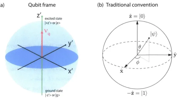
is called the qubit frequency, since huq gives the energy splitting between the two eigenstates, |+z') and |-z'). The Hilbert space is spanned by these two energy eigenbases, so the new reference frame is named the qubit eigenbasis frame or simply the qubit frame.

The "south pole -+ ground state" convention

According to Eq. (2.15), the ground (excited) state can be graphically represented

by |-z') (|+z')), or south (north) pole on a unit Bloch sphere (Fig. 2-3a). In many places in the literature, we frequently see the opposite convention, where the ground state is traditionally defined at the north pole (Fig. 2-3b). However, in terms of the Hamiltonian, it would be so if an additional minus sign is placed in Eq. (2.15). The convention historically derives from treating a spin of a negative gyromagnetic ratio, such as an electron spin, in the presence of a static magnetic field. Such system would

Qubit frame Z _{excited state} +z'> or le> (b) Traditional convention i = 10) O I %k ground state |-z'> or g>

Figure 2-3: (a) Bloch representation of a static Hamiltonian quantized along z' in the qubit frame. The ground (excited) state corresponds to the south (north) pole of the Bloch sphere. (b) The traditional convention, in which 10) at the north pole is considered as the ground state.

have a lower energy when the spin is oriented in the same way as the field. Computer scientists are also used to this convention, since they focus more on the computational indication brought by 10)'s and 1)'s than on the physical meaning.

However, throughout this thesis, we will follow the "south pole +-+ ground state" convention to circumvent the minus-sign confusion. A more natural reason for such choice is that it is more intuitive to visualize a system where the pointer of a least energized state is downwards oriented.

2.4

Radiofrequency Pulse

In this section, we will discuss how the qubit is affected by external (time-dependent) control.

A unitary gate operation is equivalent to a length-preserving (trace-preserving in

terms of density matrix) rotation of the state vector. In order to implement a qubit operation, experimentally, at least one of the parameters in the Hamiltonian has to

be modulated in either of the following ways [37]:

" (near) resonant radiofrequency (r.f.) pulses, " adiabatic pulses,

" non-adiabatic DC pulses (rise time much shorter than the characteristic

evolu-tion time).

Since only the first approach pertains to the experiments explored in this thesis, we will focus on the dynamics in the presence of resonant r.f. pulses.

Assume the same system Hamiltonian as in Eq. (2.10) but with an additional harmonic drive (Fig. 2-4):

h

7 = [ZA&z + E x + Arf cos(2xrurft + $>&x] . (2.17)

The static part of the Hamiltonian,

Nstatic

=

[A&z

+ E&X represents the qubit's internal field, while the oscillating term, Hrf = !Arf cos(2wurft + $)&x, represents the

external harmonic drive with amplitude Arf, carrier frequency (or r.f. frequency) vrf and phase $. The AC control only modulates the tunable parameter, E, so that the sinusoidal term oscillates along the x-axis.

The question is whether the AC part can produce a large effect on the qubit state, even if the oscillation is weak compared to the static field, i.e., Vrf

<

uq, and how.

First, we rewrite the Hamiltonian in Eq. (2.17) in the qubit frame (Fig. 2-4):

h

' [vquzi + Arf cos 0 cos(27rrft + $)&Xi + Arf sin 6 cos(27rvft + $)&z] . (2.18)

The second and third term on the r.h.s. represent the transverse and longitudinal perturbation to the qubit, respectively. From the perturbation theory, to effectively induce transition between the two eigenstates (I+z') and

|-z'))

requires two condi-tions,

e Transverse coupling: the perturbation is transverse, i.e., the perturbating

Laboratory frame - Qubit frame

z

I.

X

X

Figure 2-4: Bloch representation of a driven Hamiltonian in Eq. (2.17).

Frequency resonance: the perturbation is near resonant, i.e., the frequency of the perturbation, up to a Planck constant, is equivalent or very close to the energy difference between the two states.

For a TLS with harmonic drive, the resonance condition is expressed by equating the oscillation frequency to the qubit frequency:

vrf = Vl . (2.19)

The effect is analogous to its classical counterpart, e.g., periodically driving a

pendu-lum, where the swinging of the pendulum only gets significant when the frequency of

2.4.1

Rotating Frame

The motion becomes more complicated in the presence of an fast oscillating Hamilto-nian, and hard to visualize in the original 3D space. In order to conveniently describe and analyze the dynamics, a special mathematical transformation is applied. The transform is done by moving into another reference frame which revolves around the original quantization axis (z') at the r.f. frequency (vrf) [22, 35]. In fact, the transfor-mation is a special example of the interaction-picture formalism. We will show that, the Hamiltonian turns out to be time-independent again in this rotating frame with proper approximations.

The rotating-frame transformation is achieved by a time-dependent unitary trans-formation,

U = Rz(27rvfrt) , (2.20)

with corresponding coordinate transformation,

&x = cos(27rvft)&x/

+

sin(21rvrft)&y,

&y = cos(27rvrft)&y/ - sin(2,rurft)&x/ ,

0z = Uz, . _(2.21)

Following the same procedures prescribed in Eq. (2.11) and Eq. (2.12) or the interaction-picture formalism, we can derive, from the original Hamiltonian in Eq. (2.18), a rotating-frame Hamiltonian,

' = Ut'Q - hVrf&Z/2 . (2.22)

The second term on the r.h.s. is the quantum analogue of the classical inertial field that arises from transforming to a non-inertial frame. For our example, Eq. (2.22)

Qubit frame - Rotating frame ZI

IjVq

Y.

Figure 2-5: Geometric illustration of the t

{x', y', z'} and the rotating frame {X, Y, Z}.

ransformation between the qubit frame

can be explicitly expressed by

h

1N = _vz

+

1

IArf

cos O (cos

#

&x + sin# &y)

2 1

+ Arf cos 0 (cos(-2,r - 2v.ft - #)&x + sin(-2r - 2vrft - )&y)

2

+ Arf sin 6 cos(21rurft

+

#)&z]

(2.23)

where Av = V - vf is the frequency detuning between the qubit and the driving

field.

In the weak driving limit (Arf < vrf), the last two lines in Eq. (2.23) can be

omitted, since these rapid oscillations average to zero on any appreciable time scale of qubit dynamics in the rotating frame. It is known as the rotating-wave approximation

(RWA) [38], which is generally satisfied in the experiments explored in this thesis.

WY

X

The Hamiltonian after approximation is given by (Fig. 2-6)

h

7 = 2

[vz

u + v,, (cos <;b x + sin <; 6y)] , (2.24)

where vR = Arf cos 0 is the Rabi frequency (to be defined later) when the driving field is resonant with the qubit (Eq. (2.19)).

Rotating frame

z

t

~I

'X

Figure 2-6: Bloch representation of the driven Hamiltonian in the rotating frame after rotating-wave approximation.

Eq. (2.24) describes a static field but in a new reference frame. According to the

rules of state evolution (Sec. 2.2), the qubit will execute Larmor precession around the new static driving field (the Z'-axis in Fig. 2-6) in the rotating frame (choice of the reference frame does not affect dynamics as long as equations of motion are identical). Such rotating-frame precession is known as nutation in the NMR language.

The nutation is usually called Rabi precession, and the nutation frequency is named the Rabi frequency after I.I. Rabi who did the pioneering work on the effect of

a gyrating field in magnetic resonance [39]. The effective Rabi frequency in Eq. (2.24),

VR = v. 1 + /(ARiy)2 _, (2.25)

equates to vR when on-resonance. The axis of the vectorized field is tilted from the equatorial plane by an angle r; = arctan(Av/vR). For a resonant pulse, the nutation axis lies in the X-Y plane (Fig. 2-7). The pulse phase derives from the initial phase of the harmonic drive. Routinely, it is called an X-pulse if

#

= 0, or a Y-pulse if

#

=r/2.

Rotating frame

z

4

. Y

Figure 2-7: The resonantly driven Hamiltonian in the rotating frame.

In the absence of the r.f. pulse, the qubit precesses around the Z-axis at the detuning frequency

Av

in the rotating frame.

2.4.2

Single Pulse

Now, let's look at what a single r.f. pulse does to the qubit in terms of measurement. To begin with, assume the pulse is a resonant X-pulse (Av = 0,

#

= 0) and has

a square-profiled envelope (constant amplitude over duration T) (Fig. 2-8). Driven

by the Hamiltonian in Eq. (2.24), the qubit rotates around the X-axis at a constant

cycling rate of vR over the pulse duration.

Rabi

z

t

Figure 2-8: Left: single square-shaped X-pulse. Right: Rabi precession. Dashed arrows are examples of the r/2 and -r nutation, starting from the ground state.

If the qubit is initially prepared at its ground state (|-Z) = |-z')), with respect to the static Hamiltonian (Eq. (2.15)), it undergoes Rabi precession in the Y - Z plane (Fig. 2-8). A significant observation in this special example is that the qubit will coincide with the excited state periodically, suggesting an efficient way to induce population inversion. In fact, the measured population or probability of either state after this pulse is a sinusoidal function of T (Rabi oscillation), and the oscillating frequency is exactly vR. If the pulse is off-resonance, the nutation axis is tilted from the X-axis, along with tilt of the precession plane. Consequently, the population cycling becomes less complete, and the system cannot be fully excited.

For Y-pulse (# = 7r/2), the population-cycling phenomenon is identical to that of the X-pulse. Actually, the observed Rabi oscillation is the same for an arbitrary

#,

since we only measure the z'-component. This suggests that, for single pulse, the drive phase does not matter to the dynamics. In fact, because we can always choose

an arbitrary time-point as our starting time (t = 0), the initial phase can be defined

Take a look at two important examples of single pulse. If the pulse is configured such that 27rvRr = r (the total area integrated over the pulse envelope), we call it a 7r-pulse. A wr-pulse executes exactly half a Rabi cycle, so it can fully excite the qubit from the ground state to the excited state. For an arbitrary initial state, it simply mirrors the state vector against the nutation axis. For example, 7r) -pulse (subscript indicates the pulse phase) can perform the translation: |-Z) -+ |+Z), |+Y) -+ |-Y), and |+X) -+

I+X).

If the pulse is configured such that 27rvRT = 7r/2, we call it

7r/2-pulse. A ir/2-pulse executes exactly a quarter Rabi cycle, so it is used to create a superposition state from the ground state. For example, ir/2)x-pulse can perform the translation: --Z) -+ |+Y) = I+z)±i-Z). These two types of pulses are frequently used in practical experiments, and are elementary building blocks of quantum gates. The square profile of a pulse is only an ideal case. In practice, the actual pulse shape finally seen by the qubit hardly exhibits sudden rise or fall due to bandwidth limit of electronics ubiquitous at different steps (pulse generation, cable transmission, on-chip production). To make the transition smooth, a finite rise and fall time is necessary. Because the frequency response of a Gaussian pulse has a rather narrow bandwidth, the pulses used in our experiments generally have a Gaussian profile for short pulses like the 7r- and r/2-pulse, or Gaussian rise and fall (typically 5 - 10 ns

rise/fall time) for long pulses. The nutation angle by these shaped pulses is simply the total area integrated over the pulse envelope. In practice, the parameters for the 7r- or 7r/2-pulse configuration are calibrated from Rabi oscillations. That is, measure the qubit after a single pulse with either the pulse amplitude or width updated. The pulse parameters for a desired nutation angle can thus be determined from measured Rabi oscillations.

2.4.3

Multiple Pulses

What if there are multiple pulses? In Sec. 2.4.2, we already saw that a single pulse can be treated as a Rabi field which is turned on for a certain duration in the rotating frame. The combined effect from multiple pulses (same frequency) can be considered as a series of individual fields in the order of their positions over the timeline. However,

a little more attention should be paid to the complication brought by the pulse phase. Because we can only choose one frame as the reference frame, the phases of different pulses should always be referenced to a same starting time, no matter when the pulses are turned on or off. This is equivalent to saying that, if the first pulse is defined as an X-pulse (we can always do this whatever value

#

1 is, since we can choose any t

as the starting time), the pulse phase in the rotating frame of the k-th pulse is then

#k

-

#

₁. This suggests that the only important quantity is the relative phase with respect to the first pulse. For example, if

#

2 - = 1r/2, the second pulse is effectively

a Y-pulse after the first X-pulse. Also, due to the

#1

-invariance, the X-Y phase order in the two-pulse example is equivalent to Y-X or X-Y (bar indicates a 180-degrees phase-shift or negative orientation).

2.5

Free Evolution and Related Experiments

Here, free-evolution related experiments does not mean that the qubit undergoes free precession without any external control throughout the experiment. Rather, it indicates that we will only focus on decohering phenomena associated with the free-evolution or pulse-free periods within the measurement protocol. To put in another way, the desired noise information is encoded during the free-evolution periods. In fact, properly designed pulse sequences are required to manipulate the qubit so that the concerned noise processes manifest themselves in the observations.

These experiments typically consist of multiple short pulses like 7r/2- and ir-pulses, with a particular pulse-spacing setting, so that noise information is encoded in a desired way.

2.5.1

Free Evolution and Its Decoherence

Here, we discuss the qubit's decohering dynamics during free evolution. As shown in Sec. 2.3, under the internal Hamiltonian (Eq. (2.15)), the qubit undergoes free precession at the qubit frequency (vq) around the quantization axis (z') in the qubit frame. The azimuthal angle of the qubit's Bloch vector

#

depends on the initial

state. For example, if the qubit starts from the ground (--z')) or excited state

(I+z')), / = 1800 or 0'. In either case, the qubit state remains unchanged during free precession. If the qubit is initially prepared at an equal-superposition state, e.g.,

I+x')

or

|±y'),

#

= 900 and the qubit will precess around the equatorial plane. In

general, for an arbitrary value of #, the qubit leaves a cone-like trace symmetric about

z' (Fig. 2-1).

Now we include decoherence into the system by introducing an additional pertur-bative Hamiltonian,

h1

0

=

, z +

5

Oe

& X]

.(2.26)

The Hamiltonian describes the system's coupling to a noisy environment.

QA(t)

(Qe(t)) represents the fluctuating bath variable that couples to the A (F) terms. Since

E and A are physically different, QA(t) and

Q,(t)

are supposed to be uncorrelated. Also note that all fluctuations discussed in this thesis, unless otherwise specified, are zero-mean.

The noise power spectral densities (PSD), SA(f) and Se(f), are defined as the symmetrized bilateral PSD:

SA(f) = (27r)2 dt exp(-i2-rft) (A(0)A(t) + A(t)A(0)) , (2.27)

where A E {x', y', z'... or A(=

QA),

e(=

QF)

...

}

indicates either the fluctuating

part of system Hamiltonian or the axis to which those fluctuations couple. It is parametrized in units of frequency [Hz], e.g., for A originally in unit of energy [J], it is reduced by a Planck constant, i.e., A -+ A/h. The symmetrized autocorrelation function, 2(A(0)A(t) + A(t)A(0)), is equivalent to the regular autocorrelation function

(A(0)A(t)) for classical noise or quantum noise in the classical limit, i.e., hf < kB T

where kB is Boltzmann's constant and T is the temperature. For quantum noise, the expectation value is taken over the environment's ensemble state, i.e.,

(O)

=

TrE [bpE], where PE is the environment's density matrix. More discussion about the difference between the quantum and classical noise can be found in Appendix A.

When transformed into the qubit frame, the Hamiltonian in Eq. (2.26) becomes

74

= A($ Cos 0 +

Se

sin 0)&z/ + (-$A sin 9 + Qe Cos 0)&X/

h

-

($z'&zl

+

$x'x,]

. (2.28)

The A and e noise are assumed to be uncorrelated as their fluctuations have different physical origins (in the device we explored in this thesis), the PSD of the qubit-frame noise Q,1(t) or Qx,(t) is a (co)sinusoidally weighted sum of the PSD in the lab frame, namely,

Si(f ) = sin2_{0 SA(f)}

+ cos2_{0 S (f)}

SZ,(f) = cos20 Sn(f) + sin2_{o SE(f) . (2.29)}

Eq. (2.29) suggests that we are able to tune the sensitivity to lab-frame noise by

varying 9 or, physically, E. In the special case when E = 0, the laboratory frame and the qubit frame coincide and the z'-noise has no contribution from the E noise.

The evolution of this open quantum system in the Markovian weak-coupling limit can be solved by the Bloch-Redfield theory. For a general open quantum system, WS + I +

NE

(Ws, 7-I and WE stand for the system, interaction and environment Hamiltonian, respectively), the evolution of the combined system,

#(t),

in the inter-action picture,

pint

= ftp U (U = e-inst/h), is governed by the interaction-picture

Liouville-von Neumann equation,

d = [NI,int, I , _(2.30)

where

N

t= UtNU. In the rest, we omit the subscript "int" for more uncluttered expressions.

Next, making two major assumptions,

e Born approximation: the coupling is weak enough and the reservoir is big enough, so that the density matrix factorizes,

P

=

PS

@PE, and the environment