HAL Id: hal-00697240
https://hal.inria.fr/hal-00697240
Submitted on 15 May 2012
HAL is a multi-disciplinary open access
archive for the deposit and dissemination of
sci-entific research documents, whether they are
pub-lished or not. The documents may come from
teaching and research institutions in France or
abroad, or from public or private research centers.
L’archive ouverte pluridisciplinaire HAL, est
destinée au dépôt et à la diffusion de documents
scientifiques de niveau recherche, publiés ou non,
émanant des établissements d’enseignement et de
recherche français ou étrangers, des laboratoires
publics ou privés.
A Constructive Proof of Dependent Choice, Compatible
with Classical Logic
Hugo Herbelin
To cite this version:
Hugo Herbelin. A Constructive Proof of Dependent Choice, Compatible with Classical Logic. LICS
2012 - 27th Annual ACM/IEEE Symposium on Logic in Computer Science, Jun 2012, Dubrovnik,
Croatia. pp.365-374. �hal-00697240�
A Constructive Proof of Dependent Choice,
Compatible with Classical Logic
Hugo Herbelin
INRIA - PPS - Univ. Paris Diderot
Paris, France
e-mail: [email protected]
Abstract—Martin-Löf’s type theory has strong existential elim-ination (dependent sum type) that allows to prove the full axiom of choice. However the theory is intuitionistic. We give a condition on strong existential elimination that makes it computationally compatible with classical logic. With this restriction, we lose the full axiom of choice but, thanks to a lazily-evaluated coinductive representation of quantification, we are still able to constructively prove the axiom of countable choice, the axiom of dependent choice, and a form of bar induction in ways that make each of them computationally compatible with classical logic.
Keywords-Dependent choice; classical logic; constructive logic; strong existential
I. Introduction
a) Scaling Martin-Löf ’s proof of the axiom of choice to classical logic: In Martin-Löf’s intuitionistic type theory [26], the functional form of the axiom of choice has a simple proof:
ACA , λH.(λx.wit (H x), λx.prf (H x))
: ∀xA∃yBP(x, y) → ∃ fA→B∀xAP(x, f (x))
where wit and prf are the first and second projections of a strongexistential quantifier1.
The proof is constructive: it is a program which we can compute with in the sense that any closed proof of some Σ0
1-statement ∃z g(z) = 0 that uses the axiom of choice will
eventually provide with a witness t such that g(t)= 0. On the other side, classical logic is “constructive” too [17], [31] and by interpreting Peirce’s law by means of the callcc and throw control operators2, we can also compute witnesses
from closed proofs ofΣ0
1-statements.
Combining the two is however delicate. Reminding that callccαphas type A and binds the continuation variable α of input type A when p has type A while throwαp has arbitrary type B for p of type A and α of input type A, we cannot accept the following instance of the standard reduction rule for callcc in natural deduction:
prf (callccα(t1, φ(throwα(t2, p))))
. callccαprf (t1, φ(throwαprf (t2, p)))
since if the continuation α had input type ∃n P(n) in the left-hand side then it would have to have both input types P(t1)
1Also known asΣ-type, dependent sum, or strong sum.
2We use the SML names of these operators that exist also with other names
in various other programming languages.
and P(t2) in the right-hand side, leading to an unexpected
de-generacy of the domain of discourse3 [19]. This first problem
is solved by using higher-level reduction rules such as E[prf (callccα(t1, φ(throwα(t2, p))))]
. callccαE[prf (t1, φ(throwαE[prf (t2, p)]))]
E[wit (callccα(t1, φ(throwα(t2, p))))]
. callccαE[wit (t1, φ(throwαE[wit (t2, p)]))]
where the reduction is allowed only when E is an evaluation context whose return type does not depend on its hole. However, this does not help much be-cause if E contained other occurrences of the expression prf (callccα(t1, φ(throwα(t2, p)))) derived from the same
initial proof (and this is precisely what would happen in Martin-Löf’s proof of ACA if the two copies of H x were
classical proofs of the form callccα(t1, φ(throwα(t2, p)))), the
synchronisation between the two proofs would be lost. b) Realising the axioms of countable choice and depen-dent choice in the presence of classical logic: The axiom of countable choice
ACN : ∀xN∃yAP(x, y) → ∃ fN→A∀xNP(x, f (x))
and the slightly stronger axiom of dependent choice DC : ∀xA∃yAP(x, y) →
∀x0∃ fA→A( f (0)= x0∧ ∀n P( f (n), f (S (n))))
are two weak instances of the full axiom of choice and realis-ability contributed to understand their computational content in the presence of classical logic. Three approaches were followed.
A breakthrough was made in 1961 in the context of Gödel’s functional interpretation (Dialectica) with the definition by Spector [35] of a notion of bar recursion so as to realise the principle of double negation shift from which the functional interpretation of the axiom of dependent choice follows.
Much later, in 1997, a direct realiser, in a sense close to the one of Kleene [22], was proposed in the context of the arithmetic in finite types by Berardi, Bezem and Coquand [6] for the negative translation of the axiom of dependent choice. In both cases, the key ingredient is a recursive loop param-eterised by a finite portion of the function being built, each
3Failure of subject reduction when combining strong existential
quantifi-cation and computational classical logic was also observed by P. Blain Levy (private communication).
recursive call carrying one more piece of information than the preceding one, the whole process being terminating because, for the simply-typed λ-calculus based language of realisers they consider, closed programs over functions only uses a finite amount of information of their argument. Later on, Berger and Oliva [8] reformulated Berardi, Bezem and Coquand’s realiser in terms of some notion of modified bar recursion. Then, in 2004, Berger [7] reduced the termination of these realisers to some variant of open induction called update induction:
U IP : ∀ f (∀n( f (n)= ⊥ → ∀a P( f [n ← a])) → P( f ))
→ ∀ f P( f )
for f ranging over N → A⊥ for A arbitrary and A⊥ the
extension of A with one extra element ⊥, for a ranging in A and f [n ← a] denoting the function g defined by g(n)= a and g(p) = f (p) for p , n, for P( f ) open predicate of the form ∀n Q( f|n) → ∃n R( f|n) assuming that f|n is the
sequence ( f (0), ..., f (n − 1)). Otherwise said, Berger reduced the computational content of the axiom of dependent choice to a well-foundedness axiom whose computational content is a simple fixpoint. In practice, this means that we can prove the axioms of countable choice and dependent choice in a logic satisfying cut-elimination by just setting an axiom U IP whose computational content is a well-founded recursor:
U IPp f. p f (λnλqλa.UIPp f[n ← a]).
In 2003, Krivine proposed realisers for the axioms of countable choice and dependent choice [23] in the context of classical realisability for second-order arithmetic. Classical realisability, as developed by Krivine [24], can be seen as the composition of Kleene’s realisability [22] with double negation translation and Friedman-Dragalin’s A-translation4 [13], [16].
Alternatively, it can be seen as a form of realisability allowing the use of control operators in realisers. Using our notations, the variant of countable choice realised by Krivine is
AC?
N : ∀x
N∃YN→?P(x, Y) → ∃FN→N→?∀xNP(x, F(x))
where N → ? and N → N → ? respectively denote the type of predicates and relations over N. Krivine’s realiser for AC?
N does not use a fixpoint but instead a “quote” function
which, informally, maps those Yxsuch that P(x, Yx) into natural
numbers that can then be compared so that the Yx with least
“quote” is used to define F on x. The realiser also crucially uses control operators: if some Yx is found that has lesser
quoted value than the Yx currently used to build F, the
evaluation context at the time F(x) was requested is restored and a new computation of F on x with new Yx is started. In
particular, Krivine’s realisers are rather different in style from the ones of Berardi, Bezem and Coquand, and a fortiori from bar recursion. They do not seem either to generalise to choice functions with arbitrary, non relational, codomain A.
4See e.g. Berger and Oliva [8] for a notion of realisability obtained by
combination of Kleene’s realisability and Friedman-Dragalin A-translation and in which ⊥ is realisable. That Krivine’s classical realisability contains A-translation comes from the fact that ⊥ is not empty but realised by a fixed set of realisers.
c) Call-by-name, call-by-value and call-by-need: Church’s λ-calculus [9], [5] comes naturally as a “call-by-name” calculus and it is its use in computer programming languages that motivated the theoretical study of its more intricate5 call-by-value counterpart, thanks successively to Plotkin [32], Moggi [27], Sabry and Felleisen [33], Sabry and Wadler [34], etc. Similarly, call-by-need λ-calculus, which is at the heart of programming languages like Haskell [15], progressively tends to be studied at the same foundational level its call-by-name and call-by-value variants are, see [2], [25], or, in the presence of control, [29], [4], [3]. Call-by-value and call-by-need are appropriate for sharing values and will turn to be useful for dealing with theories that might reflect proofs inside terms.
d) Internalising the construction of an approximation of the choice function at the level of proofs: In order to preserve the synchronisation between different instances of proofs, that are classical and hence liable to duplicate their evaluation con-text, call-by-value evaluation is indeed appropriate. However, in the proof of the axiom of choice above, the two occurrences of H x are in the scope of different binders of x what forbids the possibility to share them.
Let us assume that the domain of quantification A is the domain of natural numbers. Let us also assume for a while that we could define the choice function and its property by infinite terms. Then we could prove the axiom of countable choice with the following infinite proof:
ACN, λH. (λn.if n = 0 then wit (H 0) else
if n= 1 then wit (H 1) else ..., λn.if n = 0 then prf (H 0) else
if n= 1 then prf (H 1) else ...) Now, we have an infinite number of calls to H but each of these calls is parameter-free and hence shareable. Using the let operator of call-by-value, we can then make sharing explicit:
ACN, λH. let H0= H 0 in
let H1= H 1 in
...
(λn.if n= 0 then wit H0 else
if n= 1 then wit H1 else...,
λn.if n = 0 then prf H0 else
if n= 1 then prf H1 else...)
Now we have to capture the infinity by finitary means and this is possible by turning the infinite sequence of let into a single stream definition (H 0, H 1, ...). This leads to the following proof of the countable axiom of choice:
ACN, λH. let s = cofix 0
f n(H n, f n) in
(λn.wit (nth n s), λn.prf (nth n s)) where cofix0f n(H n, f n) is a corecursive definition of the stream iterating on f with parameter n and started at 0
5Though, when looking at λ-calculus from the point of view of sequent
calculus instead of from the point of view of natural deduction [12], [18], call-by-value λ-calculus gets no more complicated than call-by-name, both having the same - intermediate - level of intrinsic technical complexity.
while nth n s is a recursive definition of the access to the nth component of the stream s.
At the level of formulae, the stream is an inhabitant of a coinductively defined infinite conjunction ν0Xn(∃y P(0, y)∧X(n+ 1)). At the level of computation, since a stream is infinite, we cannot afford evaluating each of its component in advance, so we have to use a lazy call-by-value mechanism.
e) Outline: To make a sound formal system of this analysis, it remains to characterise the restriction required on strong existential elimination so that it becomes compatible with classical logic. In Section II, we study this restriction in the classical arithmetic in finite types, showing in passing how to define coinductive formulae in this context. By lazy evaluating the coinductive proofs, termination can reasonably be claimed, from which conservativity of classical logic over intuitionistic logic for Σ0
1 formulae in the presence of strong
existential elimination entails. In Section III, we show how to exploit the coinductive connectives to give a proof of the axioms of countable choice, axiom of dependent choice, and bar induction. Open issues will be discussed in Section IV together with a comparison with some other works.
II. dPAω: Classical Arithmetic in Finite Types with Strong Existential
We now focus on the arithmetic in finite types and extend dPL with quantification over functions of higher-order types and recursion. In this logic, that we call dPAω, the axioms of countable choice and dependent choice can be proved as will be shown in the next section.
Even though coinductive formulae can be defined in dPAω, thanks to the quantification over functions, we will consider a primitive notion of coinductive formulae, considered positive, and that will be precisely convenient for proving the axioms of countable choice and dependent choice.
A. Proofs and Terms
Strong existential elimination forces formulae to be depen-dent of proofs. In dPAω, terms t, u, ... can depend on proofs
p, q, ..., and vice versa so that both are defined mutually: t, u ::= x | 0 | S (t) | rec t of [t | (x, y).t] | λx.t | t t | wit p p, q ::= a | ιi(p) | (p1, p2) | (t, p) | λa.p | λx.p | case p of [a1.p1| a2.p2] | split p as (x, a) in q | dest p as (x, a) in q | prf p | p q | p t | exfalso p | refl | subst p q | ind t of [p | (x, a).q] | cofixtbxp | catchαp | throwαp | let a= p in q
where f ranges over function symbols, ~t denotes in f (~t) a sequence of terms of length the arity of f , the names x, y, . . . range over a set of term variables, a, b, . . . over a set of proof variables, α, β, . . . over a set of continuation
variables. The constructions λa.p, case p of [a1.p1| a2.p2],
split p as (a1, a2) in q, dest p as (x, a) in q and
ind t of [p | (x, a).q] bind a, a1 and a2. The constructions
λx.p, dest p as (x, a) in q, dest p as (x, a) in t, λx.t, ind t of [p | (x, a).q] and rec t of [t | (x, y).t] bind x and y. The construction catchαpbinds α. The binders are considered up to the actual name used to represent the binder (α-conversion) and the set of free variables FV(p) of a proof p is, as usual, the set of variables of p that are not bound inside p itself.
Most constructions speak by themselves with the peculiarity that terms can be built by case analysis (case) or destruction of proofs (split and dest). The operator rec t of [t | (x, y).t] is for recursion in finite types while ind t of [p | (x, a).q] is for induction. The construction cofixtbxp is for building coinductive formulae.
Let us say also that the operators catch and throw im-plement classical reasoning. They are similar to the operators of same name in Nakano [28] or Crolard [11]. In terms of Parigot’s λ-calculus [30], catchαp is basically equivalent to µα.[α]p and throwαp to µδ.[α]p for δ not occurring in p.
The abbreviations π1(p), split p as (a1, a2) in a1 and
π2(p) , split p as (a1, a2) in a2 might occasionally be
useful.
To emphasise that a term variable ranges over functions, we might use symbols derived from the letters f or g instead of xor y. We might also use n or m for a variable ranging over natural numbers.
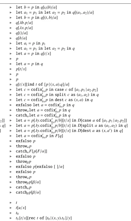
B. Operational Semantics
We equip dPAω with a call-by-value evaluation semantics and for that, a subclass of proofs will play a particular role in extracting the intuitionistic content of positive formulae. These are the values defined by:
V ::= a | ιi(V) | (V, V) | (t, V) | λa.p | λx.p | () | refl
To define the operational semantics of dPAω, we also need to define the class of elementary call-by-value evaluation contexts. Because of corecursion, we have potentially infinite values and we do not want to fully reduce proofs using a call-by-value semantics. Therefore, we use an incremental reduc-tion semantics which is lazy on the evaluareduc-tion of corecursive values. Lazy evaluation requires to introduce specific contexts, written D, which accumulate pending delayed computation of cofixpoints. Altogether, evaluation contexts are defined as follows: F[ ] ::= ιi([ ]) | ([ ], p) | (V, [ ]) | (t, [ ]) | case [ ] of [a1.p1| a2.p2] | split [ ] as (a1, a2) in q | dest [ ] as (x, a) in p | prf [ ] | [ ] q | [ ] t | let a= [ ] in q | subst [ ] p D[ ] ::= [ ] | D[F[ ]] | let a = cofixtbxp in D[ ] For F[ ] an elementary call-by-value evaluation context and p a proof, we write F[p] for the proof obtained by plugging p into the hole of F[ ] and similarly for D[ ].
let a= ιi(p) in q . let b = p in q[ιi(b)/a]
let a= (p1, p2) in q . let a1= p1in let a2= p2in q[(a1, a2)/a]
let a= (t, p) in q . let b = p in q[(t, b)/a] let a= λb.p in q . q[λb.p/a]
let a= λx.p in q . q[λx.p/a] let a= () in q . q[()/a] let a= b in q . q[b/a]
case ιi(p) of [a1.p1| a2.p2] . let ai= p in pi
split (p1, p2) as (a1, a2) in q . let a1= p1in let a2= p2in q
dest (t, p) as (x, a) in q . let a = p in q[t/x] prf (t, p) . p (λa.q) p . let a = p in q (λx.p) t . p[t/x] subst refl p . p ind 0 of [p | (x, a).q] . p
ind S (t) of [p | (x, a).q] . q[t/x][ind t of [p | (x, a).q]/a] case cofixt
bxp of[a1.p1| a2.p2] . let c = cofixtbxp in case c of[a1.p1| a2.p2]
split cofixtbxp as (a1, a2) in q . let c = cofixtbxp in split c as(a1, a2) in q
dest cofixtbxp as(x, a) in q . let c = cofixtbxp in dest c as(x, a) in q let a= cofixtbxp in exfalso q . exfalso let a = cofixtbxp in q
let a= cofixtbxp in throwαq . throwαlet a= cofixtbxp in q
let a= cofixtbxp in catchαq . catchαlet a= cofixtbxp in q
let a= cofixtbxp in D[case a of [a1.p1| a2.p2]] . let a = p[λy.cofixybxp/b][t/x] in D[case a of [a1.p1| a2.p2]]
let a= cofixtbxp in D[split a as (a1, a2) in q] . let a = p[λy.cofixybxp/b][t/x] in D[split a as (a1, a2) in q]
let a= cofixtbxp in D[dest a as (x, a0) in q] . let a = p[λy.cofixybxp/b][t/x] in D[dest a as (x, a0) in q] F[let a= cofixtbxp in q] . let a = cofixtbxp in F[q]
F[exfalso p] . exfalso p F[throwαp] . throwαp
F[catchαp] . catchαF[p[F/α]] exfalso exfalso p . exfalso p exfalso throwβp . throwβp
exfalso catchβp . exfalso p[exfalso [ ]/α] throwβexfalso p . exfalso p
throwβthrowαp . throwαp
throwβcatchαp . throwβp[β/α]
catchαthrowαp . catchαp
catchβcatchαp . catchβp[β/α]
wit (t, p) . t
(λx.t) u . t[u/x] rec 0 of [t0| (x, y).tS] . t0
rec S (t) of [t0| (x, y).tS] . tS[t/x][rec t of [t0| (x, y).tS]/y]
Fig. 1. Reduction rules on terms and proofs of dPAω
The reduction rules are shown in Figure 1 where the substitutions p[V/a], p[u/x], t[V/a], t[u/x] and p[β/α] are capture-free with respect to the three kinds of variables (x, a and α) and where the substitution p[F/α] means replacing subterms of the form throwαqin p by throwαF[q] (including
the recursive replacements in q)6.
We write .. for the reflexive-transitive closure of .. We write ≡ for the reflexive-symmetric-transitive closure of ..
6Strictly speaking, the definition of p[β/α] and p[F/α] requires also to
consider their variants t[β/α] and t[F/α] on terms
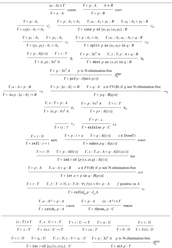
C. Types, Formulae and Inference Rules
Terms are simply typed, with the natural numbers as base type. Finite types are thus defined by:
T, U ::= N | T → U
In dPAω, we consider implication to be possibly dependent in its antecedent and use the notation [a : A] → B to express this dependency, underlining the fact that a can occur in some term in B. An advantage of allowing this dependency is the ability to express statements such as [a : ∃x P(x)] →
(a : A) ∈Γ Γ ` a : A axiom Γ ` p : A A ≡ B Γ ` p : B conv Γ ` p : Ai Γ ` ιi(p) : A1∨ A2 ∨i I Γ ` p : A1∨ A2 Γ, a1: A1` p1: B Γ, a2: A2` p2: B Γ ` case p of [a1.p1| a2.p2] : B ∨E Γ ` p1: A1 Γ ` p2: A2 Γ ` (p1, p2) : A1∧ A2 ∧I Γ ` p : A1∧ A2 Γ, a1: A1, a2: A2` q : B Γ ` split p as (a1, a2) in q : B ∧E Γ ` p : A[t/x] Γ ` t : T Γ ` (t, p) : ∃xTA ∃I Γ ` p : ∃xTA Γ, x : T, a : A ` q : B Γ ` dest p as (x, a) in q : B ∃E Γ ` p : ∃xTA p is N-elimination-free Γ ` prf p : A[wit p/x] ∃prfE Γ, a : A ` p : B Γ ` λa.p : [a : A] → B →I Γ ` p : [a : A] → B Γ ` q : A a < FV(B) if q not N-elimination-free Γ ` p q : B[q/a] →E Γ, x : T ` p : A Γ ` λx.p : ∀xTA ∀I Γ ` p : ∀xTA Γ ` t : T Γ ` p t : A[t/x] ∀E Γ ` () : > >I Γ ` p : ⊥ Γ ` exfalso p : C ⊥E Γ ` t : N Γ ` refl : t = t refl Γ ` p : t = u Γ ` q : A[t/x] x < Dom(Γ) Γ ` subst p q : A[u/x] subst Γ ` t : N Γ ` p : A[0/x] Γ, x : T, a : A ` q : A[S (x)/x]
Γ ` ind t of [p | (x, a).q] : A[t/x] ind Γ ` p : A Γ, a : A ` q : B a < FV(B) if p not N-elimination-free
Γ ` let a = p in q : B[p/a] cut Γ ` t : T Γ, f : T → N, x : T, b : ∀y f (y) = 0 ` p : A f positive in A
Γ ` cofixt bxp: ν t f xA νI Γ, α : A⊥⊥ ` p : A Γ ` catchαp: A catch Γ ` p : A (α : A⊥⊥) ∈Γ Γ ` throwαp: C throw (x : T ) ∈Γ Γ ` x : T Γ, x : U ` t : T Γ ` λx.t : U → T Γ ` t : U → T Γ ` u : U Γ ` t u : T Γ ` 0 : N Γ ` t : N Γ ` S (t) : N Γ ` t : N Γ ` t0: U Γ, x : N, y : U ` tS : U Γ ` rec t of [t0| (x, y).tS] : U Γ ` p : ∃xTA pis N-elimination-free Γ ` wit p : T ∃witE
P(wit a))7. In addition to the usual connectives and quantifiers, we have coinductive formulae:
A, B ::= t = u | [a : A] → B | A ∨ B | A ∧ B | ⊥ | > | ∀xTA | ∃xTA |νt
f xA
In atoms, P ranges over predicate symbols and ~t is a sequence of terms whose length is the arity of P. Negation ¬A is defined as A → ⊥. The construction νt
f xAstands for the instance on t
of the coinductive predicate built from the monotone functor λ f.λx.A where A is made of atoms and positive connectives only (including ν-formulae themselves). In ∀x A and ∃x A, x is bound and freely subject to renaming (α-conversion). In νt
f xA,
x and f are bound term variables. The formulae ∀x A and [a : A] → B are called negative. All other kinds of formulae are called positive.
Formulae are considered modulo the equational theory on terms, as it is common in Martin-Löf’s intensional type theory. The equational theory is the one induced by reduction on terms and proofs plus the following reduction rules for equality8and coinductive formulae unfolding:
0= 0 . > 0= S (u) . ⊥ S(t)= 0 . ⊥ S(t)= S (u) . t = u νt f xA . A[t/x][ν y f xA/ f (y) = 0]
We write ≡ for the resulting9 reflexive-symmetric-transitive closure of . on formulae.
When obvious from the context, or not relevant, we may occasionally drop the type of the variable in the quantifiers.
Since there are terms in all finite types in dPAω, it is convenient to indicate the types of variables in typing contexts. Hence, contexts are defined by:
Γ ::= ∅ | Γ, x : T | Γ, a : A | Γ, α : A⊥⊥
where a : A stands for an assumption of A and α : A⊥⊥ for an assumption of the refutation10 of A (with the objective of obtaining a proof by contradiction). On its side, x : T stands for the declaration of a variable of type T . It is assumed that assumptions have distinct variable names and we write Dom(Γ) for the set of names a and α thus declared in Γ.
Inference rules are given in Figure 2 with the typing rules in the bottom. The main difference with ordinary logic is the strong elimination rule of existential quantification and the appropriate support for formulae depending on proofs.
7We do not get extra logical strength from this design choice. It can be
proved in the case of predicate logic that the logic with dependent implication is conservative over ordinary predicate logic and we conjecture that dPAω with dependent implication is conservative over its version without dependent implication.
8See e.g. Allali [1] for such a presentation of arithmetic.
9Unfolding of coinductive formulae makes the reduction system non
terminating. One might wonder if it would make ≡ undecidable: no, because unfolding can just be used lazily.
10Not to be confused with the notation ABsometimes used for powerset.
In the rule νI, the function f is said to be positive in A if A
is built from atoms11 f(t)= 0 using disjunction, conjunction, existential quantification, equality or another coinductive type. That the typing rule νI and the reduction rule for coinductive
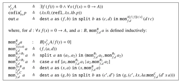
formulae do not extend by themselves the logical strength of HAω and PAω comes from the equations given in Figure 3 where out a implements the reduction rule for νt
f xA. However,
the derived computational content is not the one we want because of the use of non positive connectives in the second-order encoding, what justifies taking νI and its associated
reduction rule as primitive. Indeed, with a primitive notion of coinductive formula, it becomes syntactically direct to see ν as a constructor of positive formulae. In particular, and this is important later on to prove the axioms of countable choice and dependent choice, strong existential elimination is allowed to descend through coinductive formulae.
Dependent proofs have to be N-elimination-free (negative-elimination-free). N-elimination-freeness is defined by the following rules:
• a, (), λx.p and λa.p are N-elimination-free
• if p, q, p1 and p2 are N-elimination-free then
ιi(p), (p1, p2), (t, p), case a of [a1.p1| a2.p2],
split q as (a1, a2) in p, dest q as (x, a) in p,
prf p, refl, subst p q, ind t of [p1| (x, a).p2] and
let a= p in q are N-elimination-free.
Otherwise said, in N-elimination-free proofs, expressions of the form p q, p t, exfalso p, catchαp or throwαpcan only
occur in the body of a λx or of a λa.
The N-elimination-free condition is what ensures in partic-ular that wit will never be applied to a classical proof, i.e. to a proof starting with catchαpor throwαp.
The resulting theory is then essentially Troelstra’s arithmetic in all finite types HAω (with equality on N) extended with classical logic and strong existential elimination. We write dHAω for the version of dPAω with rules catch and throw removed. Since dPAω has classical reasoning, quantification over functional symbols and, as will be shown in Section III, dependent choice, it can simulate quantification over the predicates talking about N (since from the classical state-ment ∀n ∃b (b = 0 ∧ φ(n)) ∨ (b = 1 ∧ ¬φ(n)), we get a characteristic function f for φ, i.e. a function that satisfies ∀n ( f (n) = 0 ∧ φ(n)) ∨ ( f (n) = 1 ∧ ¬φ(n))). However, to get quantification over predicates talking about larger domains than N, one would also typically need the axiom of unique choice12 on arbitrary large domains
∀xT∃!n P(x, n) → ∃ f ∀xTP(x, f (x)) and there is no reason to think that this holds.
We are now ready to state the operational and logical properties of dPAω.
Theorem 1 (Subject reduction): IfΓ ` p : A and p . q then Γ ` q : A.
11Since we have symbols for functions and not for predicates, we use
expressions of the form f (t)= 0 to represent arbitrary atoms.
νt
f xA , ∃ f ( f (t) = 0 ∧ ∀x ( f (x) = 0 → A))
cofixtbxp , (λx.0, (refl, λx.λb.p))
out a , dest a as ( f, b) in split b as (c, d) in monA[ f / f ][t/x]f,d (d t c) where, for d : ∀x f (x)= 0 → A, and a : B, monB
f,da is defined inductively:
monBf,da : B[νyf xA/ f (y) = 0] monff,d(t)=0a , ( f, (a, d)) monB1∧B2
f,d a , split a as (a1, a2) in (monBf,d1 a1, monBf,d2 a2)
monB1∨B2
f,d a , case a of [a1.monBf,d1 a1| a2.monBf,d2 a2]
mon∃x B
f,d a , dest a as (x, a) in (x, monBf,da)
monν
u gyC
f,d a , dest a as (g, b) in split b as (c0, d0) in (g, (c0, λx.λa.monCf,d(d0x a)))
Fig. 3. Derivability of introduction and reduction of coinductive formula
Proof: Most reduction rules are standard in a call-by-value setting with control and a simple analysis shows that they preserve the correctness of derivations. The difficulty comes from strong existential elimination. The N-elimination-freeness of p in prf p then ensures that the cases where F is prf [ ] in those reduction rules that explicitly mention F cannot happen. In particular, the only rule involving prf is prf (t, p) . p which preserves the correctness of derivations. Note also that N-elimination-freeness is stable by substitution of values.
We claim normalisation by giving a sketch of proof. Claim 1 (Normalisation): IfΓ ` p : A then p is normalis-able.
Proof: (sketch) We follow the ideas of [10] and interpret proofs in infinitary logic. Normal proofs expand into well-founded infinitary trees up to the presence of infinite branches coming from the expansion of cofixpoints and such that, beyond some given depth, only introduction rules of positive connectives occur. Otherwise said, along all branches, in-finitely many nested introduction rules of positive connectives can occur but only finitely many nested elimination rules can be found. Let us consider a minimal proof having an infinite reduction sequence. Such an infinite reduction sequence can be seen as an infinite interaction between the immediate normal subproofs of the given proof. Laziness of cofixpoint unfolding now ensures that any time an infinite branch is explored in its part made only of introduction rules, nested elimination rules of another branch are explored simultaneously. If nested elimination rules of arbitrary depths are explored, then, by dependent choice, there is an infinite sequence of nested elimination rules. This is not the case, hence, only a finite portion of the infinite branches can be explored. Therefore, the infinite reduction sequence can be turned into an infinite interaction between modified proofs obtained by artificially cutting at some large enough occurrences the infinite branches of the original interacting normal subproofs. Such modified proofs are well-founded. But using the result of [10], inter-action between well-founded normal proofs in infinitary logic necessarily terminates, a contradiction.
Theorem 2 (Conservativity, first version): If A is a closed ∀-→-ν-wit-free formula then ` p : A in dPAω implies that there is some V such that ` V : A in HAω.
Proof:Our choice of rules makes that any closed proof of Aeventually produces, by normalisation, either an expression D[V] or an expression catchαD[V] where D is made only of nested let a= cofixtbxq in [ ] (the case exfalso D[V] cannot happen because there is no value of type ⊥, the cases D[cofixtbxq] and catchαD[cofixtbxq] cannot happen because
A is ν-free, all other possible configurations are reducible since p is closed). Now, because A is ∀-→-ν-wit-free, V does not contain any subexpression of the form λa.q or λx.q. In particular, in the catchαD[V] case, it does not contain any
occurrences of α. Similarly, no variable that is bound to some cofixtbxq in D can occur in V since otherwise V would have ν in its type. Hence V is closed and is a proof of A. Since V does not contain any catch, nor throw, nor prf, it is in HAω.
In arithmetic, anyΣ0
1-formula is equivalent to a
∀-→-ν-wit-free formula. Hence we have:
Theorem 3 (Conservativity, second version): If A is Σ01 then ` p : A in dPAω implies ` p : A in HAω.
This of course implies consistency:
Theorem 4 (Consistency): 0 p : ⊥ in dPAω.
III. The Axioms of Countable Choice and Dependent Choice Our main result is that dPAωproves the axiom of countable choice, the axiom of dependent choice, and thus equivalent axioms such as bar induction, open induction and update induction. The main trick is to turn a proof of ∀xTA(x)
where possibly the proof of A(t) is classical into a coinductive conjunction A(g(0)) ∧ A(g(1)) ∧ A(g(2)) . . . for a suitable law g of type N → A, so that the coinductive stream can be reduced using a (lazy) call-by-value discipline and the resulting (non-classical) values be shared by calls to the strong existential elimination.
A. The Axiom of Countable Choice
Here, A(x) is ∃y P(x, y) and the appropriate stream we want to build is the stream A(0) ∧ A(1) ∧ A(2) . . ., so we consider
the coinductive conjunction RC(n), νnf x(A(x) ∧ f (S (x))= 0).
The proof is now direct:
ACN , λa.let b = cofix0bn(a n, b (S (n))) in (λn.wit (nthCn b), λn.prf (nthCn b)) : ∀n∃y P(n, y) → ∃ f ∀n P(n, f (n)) where nthCn : RC(0) → RC(n) nthCn , λb.π1(ind n of [b | (m, c).π2(c)])
Note that the proof does not use classical logic and holds also in dHAω.
B. The Axiom of Dependent Choice
Here again, A(x) is ∃y P(x, y) and the appropriate stream we want to build is the stream A(x0) ∧ A(g(x0)) ∧ A(g2(x0)) . . .
where g is the choice function implicit in some proof of ∀x ∃y P(x, y). So we consider the coinductive formula RD(z),
νz
f x∃y (P(x, y) ∧ f (y)= 0). The proof is now direct:
DC , λa.λx0.let b = s a x0in (λn.wit (nthDn(x0, b)), (refl, λn.π1(prf (prf (nthDn(x0, b)))))) : ∀x∃y P(x, y) → ∀x0∃ f ( f (0)= x0∧ ∀n P( f (n), f (S (n)))) where nthDn : ∃x RD(x) → ∃x RD(x) nthDn , λb.ind n of [b | (m, c).(wit (prf c), π2(prf (prf c)))] s a x : RD(x) s a x , cofixx
bn(dest a n as (y, c) in (y, (c, by)))
Note that this proof too does not use classical logic and holds in dHAω.
C. Bar Induction
To express bar induction, we extend dPAω with a type constructor for finite sequences:
T ::= . . . | T∗
t, l ::= . . . | hi | l ? t | rec l of [t | (x, y, z).t] p ::= . . . | ind l of [p | (x, y, a).p]
The corresponding reduction, inference and typing rules are canonical and we skip them.
To state bar induction, we also need to define the initial segment of length n of a function f from N to T :
f|n, rec n of [hi | (m, l). l ? f (m)]
We now have all the ingredients to state the standard formu-lation of bar induction in intuitionistic logic:
BI: ∀ f ∃n B( f|n) → ∀P
∀l (B(l) → P(l)) ∧ ∀l (∀x P(l? x) → P(l))
! → P(hi) Let us consider a contrapositive variant of BI
BIc: νhigl(¬B(l) ∧ ∃x g(l ? x)= 0) → ∃ f ∀n ¬B( f|n)
where we have recognised the negation of the conclusion as a coinductive positive formula. By classical reasoning and the axiom of unique choice, BI and BIC are equivalent.
Let us write RBI(l) for the coinductive formula occurring in
the statement of BIC. The same way as we proved the axiom
of dependent choice, we have:
BIC+ , λa.(λn.wit (π2(prf (nthBIn(hi, a)))),
λn.(wit (nthBIn(hi, a)),
(π1(prf (nthBIn(hi, a))), e a n))) : RBI(hi) → ∃ f ∀n ∃l (¬B(l) ∧ l= f|n) where nthBIn : ∃l RBI(l) → ∃l RBI(l) nthBIn , λb.ind n of [b | (m, c).(wit c ? wit (π2(prf c)), prf (π2(prf c)))]
e a n : wit (nthBIn(hi, a))=
(λn.wit (π2(prf (nthBIn(hi, a)))))|n
e a n , ind n of [refl | (m, c).subst c refl] from which BIc directly follows. Then, from BIc, we get the
following weaker form of BI: ∀ f ∃n B( f|n) → ∀g" ∀l (B(l) → g(l)= 0) ∧ ∀l (∀x g(l? x)= 0 → g(l) = 0) ! → g(hi)= 0 # Finally, in the special case when x ranges over N, the characteristic function g of any predicate P over N∗ can be built classically using the axiom of countable choice. Hence a (classical) proof of BI is obtainable in this case.
IV. Discussion and Relation to Other Works f) A constructive intuitionistic logic which proves Markov’s principle, the double negation shift and the axiom of dependent choice: It has been shown that adding delimited classical logic to intuitionistic logic allows to derive weakly classical schemes such as Markov’s principle and the double negation shift while still preserving the disjunction and exis-tence properties that are specific to intuitionistic logic [20], [21]. Adding strong existential elimination to intuitionistic logic with delimited classical logic should provide with a constructive intuitionistic logic that proves Markov’s principle, the double negation shift and the axiom of dependent choice, and that is therefore adequate for intuitionistic analysis.
g) Relation with Berardi, Bezem and Coquand’s realiser of the axiom of countable choice: The computational content of our proof of the countable axiom of choice is slightly different from the one of the realiser given in the paper by Berardi, Bezem and Coquand [6]. First, in our proof, there is no construction of a function with dummy values: when the value of a function is needed (typically because some computation with the value ends into a natural number that serves in an induction step), it is directly the (first) value given by the proof of ∀n∃y P(n, y) which is used. Secondly, in our proof, the order in which the proofs of ∀n∃y P(n, y) are evaluated is the natural order, while in the case of [6], these proofs are evaluated on demand depending on which n’s
the context that interacts with the realiser of ∃ f ∀n P(n, f (n)) needs a certification that P(n, f (n)) holds. In this sense, our proof seems suboptimal. For instance, if only the content of the proof of ∃y P(1001, y) is needed, it will evaluate all the proofs of ∃y P(n, y) for n < 1001 first. Of course, one could be more lazy than we did in our evaluation algorithm and in particular be lazy on the evaluation of each ∃y P(n, y) that is not explicitly required. Still, the stream built will be a stream of length 1001 while in [6], the stream has the same size as the number of n’s for which a proof of ∃y P(n, y) is needed.
h) Dependent choice in a logic with quantification over second-order predicates: Our approach is uniform over the type of the codomain of the choice function, so it directly scales to quantification over second-order predicate. Let us call dPA2 and dHA2 the classical and intuitionistic systems
obtained by replacing the quantification over functions in finite types with quantification over second order predicates, i.e. the systems obtained from dPAω and dHAω by replacing the definition of types with:
T, U ::= N | ? | N → T
where ? denotes the type of propositions. Then, the axiom of countable choice is provable in dPA2and dHA2, what typically
covers the instance AC?
N: ∀n
N∃YN→?P(n, Y) → ∃FN→N→?∀nNP(n, F n)
that we discuss in the next paragraph.
i) Comparison with Krivine’s realiser of the axiom of countable choice: Krivine [23] realises the axiom of countable choice13 in the context of classical second-order arithmetic
us-ing a notion of classical realisability that interprets quantifiers by intersection types and that consequently keeps no trace of the quantifiers in the realiser. A detailed comparison can be found in [20].
j) Functional interpretation and products of selection functions: Products of selection functions have been developed by Escardó and Oliva in the context of functional interpretation to interpret bar recursion [14]. This seems to correspond at the level of realisability to what we are doing at the level of proofs.
V. Conclusion
We showed how to slightly restrict strong existential elimi-nation (Martin-Löf’s dependent sum type) so that it becomes compatible with classical reasoning in a computationally sound way. In this restricted framework, we lose the full axiom of choice but keep the axioms of countable choice and dependent choice thanks to a detour via coinductively defined connectives. Because the choice functions we are able to build are paths in coinductive trees, we suspect our framework to exactly capture the strength of the axiom of dependent choice. The idea here is to reason by induction on the structure of the
13In practise, Krivine realises the axiom
CAC: ∃ZN→N→?∀nN(P(n, Z n) → ∀YN→?P(n, Y))
which is classically equivalent to ACN over the codomain N → ?.
argument of strong existential elimination, but we leave this for future work.
Acknowledgements
Concepts coming from the programming languages side were instrumental for this work and I’m grateful to the community that designed them.
On a personal side, I thank Danko Ilik, Paul-André Mel-liès, Guillaume Munch–Maccagnoni, and Noam Zeilberger for fruitful discussions they shared with me.
References
[1] L. Allali, “Algorithmic equality in heyting arithmetic modulo,” in TYPES 2007, Revised Selected Papers, ser. LNCS, M. Miculan, I. Scagnetto, and F. Honsell, Eds., vol. 4941. Springer, 2007, pp. 1–17.
[2] Z. Ariola and M. Felleisen, “The call-by-need lambda calculus,” J. Funct. Program., vol. 7, no. 3, pp. 265–301, 1993.
[3] Z. M. Ariola, P. Downen, H. Herbelin, K. Nakata, and A. Saurin, “Classical call-by-need sequent calculi: The unity of semantic artifacts,” in Fuji International Symposium on Functional and Logic Programming (FLOPS ’12), Kobe, Japan, May 23-25, 2012, 2012, to appear. [4] Z. M. Ariola, H. Herbelin, and A. Saurin, “Classical call-by-need and
duality,” in Typed Lambda Calculi and Applications - 10th International Conference, TLCA 2011, Novi Sad, Serbia, June 1-3, 2011. Proceedings, ser. Lecture Notes in Computer Science, C.-H. L. Ong, Ed., vol. 6690. Springer, 2011, pp. 27–44.
[5] H. P. Barendregt, The Lambda Calculus: Its Syntax and Semantics. Amsterdam: North Holland, 1984.
[6] S. Berardi, M. Bezem, and T. Coquand, “On the computational content of the axiom of choice,” J. Symb. Log., vol. 63, no. 2, pp. 600–622, 1998.
[7] U. Berger, “A computational interpretation of open induction,” in Pro-ceedings of LICS 2004. IEEE Computer Society, 2004, p. 326. [8] U. Berger and P. Oliva, “Modified bar recursion,” BRICS, University of
Aarhus, Denmark, Tech. Rep. 02/14, Apr. 2002.
[9] A. Church, “A set of postulates for the foundation of logic,” Annals of Mathematics, vol. 2, pp. 33, 346–366, 1932.
[10] T. Coquand, “A semantics of evidence for classical arithmetic,” J. Symb. Log., vol. 60, no. 1, pp. 325–337, 1995.
[11] T. Crolard, “A confluent lambda-calculus with a catch/throw mecha-nism,” J. Funct. Program., vol. 9, no. 6, pp. 625–647, 1999.
[12] P.-L. Curien and H. Herbelin, “The duality of computation,” in Pro-ceedings of ICFP 2000, ser. SIGPLAN Notices 35(9). ACM, 2000, pp. 233–243.
[13] A. G. Dragalin, “New kinds of realizability and Markov’s rule,” Soviet Mathematical Doklady, vol. 251, pp. 534–537, 1980.
[14] M. H. Escardó and P. Oliva, “Computational interpretations of analysis via products of selection functions,” in CIE, ser. Lecture Notes in Computer Science, F. Ferreira, B. Löwe, E. Mayordomo, and L. M. Gomes, Eds., vol. 6158. Springer, 2010, pp. 141–150.
[15] J. H. Fasel, P. Hudak, S. Peyton Jones, and P. W. (editors), “Haskell special issue,” SIGPLAN Notices, vol. 27, no. 5, May 1992.
[16] H. Friedman, “Classically and intuitionistically provably recursive func-tions,” in Higher Set Theory, ser. Lecture Notes in Mathematics, D. S. Scott and G. H. Muller, Eds. Berlin/Heidelberg: Springer, 1978, vol. 669, pp. 21–27.
[17] T. G. Griffin, “The formulae-as-types notion of control,” in Conf. Record of POPL ’90. ACM Press, New York, 1990, pp. 47–57.
[18] H. Herbelin, “C’est maintenant qu’on calcule: au cœur de la dualité,” Habilitation thesis, University Paris 11, Dec. 2005.
[19] ——, “On the degeneracy of sigma-types in presence of computational classical logic,” in Proceedings of TLCA 2005, ser. LNCS, P. Urzyczyn, Ed., vol. 3461. Springer, 2005, pp. 209–220.
[20] ——, “An intuitionistic logic that proves Markov’s principle,” in Pro-ceedings of LICS 2010. IEEE Computer Society, 2010, pp. 50–56. [21] D. Ilik, “Preuves constructives de complétude et contrôle délimité,” PhD,
École Polytechnique, 2010.
[22] S. C. Kleene, “On the interpretation of intuitionistic number theory,” The Journal of Symbolic Logic, vol. 10, no. 4, pp. 109–124, 1945. [23] J.-L. Krivine, “Dependent choice, ‘quote’ and the clock,” Theor. Comput.
[24] ——, “Realizability in classical logic,” Panoramas et synthèses, 2004, to appear.
[25] J. Maraist, M. Odersky, and P. Wadler, “The call-by-need lambda calculus,” J. Funct. Program., vol. 8, no. 3, pp. 275–317, 1998. [26] P. Martin-Löf, “A theory of types,” University of Stockholm, Tech. Rep.
71-3, 1971.
[27] E. Moggi, “Computational lambda-calculus and monads,” Edinburgh Univ., Tech. Rep. ECS-LFCS-88-66, 1988.
[28] H. Nakano, “A constructive formalization of the catch and throw mechanism,” in Proceedings of LICS 1992. IEEE Computer Society, 1992, pp. 82–89.
[29] C. Okasaki, P. Lee, and D. Tarditi, “Call-by-need and continuation-passing style,” Lisp and Symbolic Computation, vol. 7, no. 1, pp. 57–82, 1994.
[30] M. Parigot, “Free deduction: An analysis of "computations" in classical logic.” in Proceedings of LPAR, ser. LNCS, A. Voronkov, Ed., vol. 592. Springer, 1991, pp. 361–380.
[31] ——, “Lambda-mu-calculus: An algorithmic interpretation of classical natural deduction,” in Proceedings of LPAR ’92. Springer-Verlag, 1992, pp. 190–201.
[32] G. D. Plotkin, “Call-by-name, call-by-value and the lambda-calculus,” Theor. Comput. Sci., vol. 1, pp. 125–159, 1975.
[33] A. Sabry and M. Felleisen, “Reasoning about programs in continuation-passing style,” Lisp and Symbolic Computation, vol. 6, no. 3-4, pp. 289–360, 1993.
[34] A. Sabry and P. Wadler, “A reflection on call-by-value,” ACM Trans. Program. Lang. Syst., vol. 19, no. 6, pp. 916–941, 1997.
[35] C. Spector, “Provably recursive functionals of analysis: A consistency proof of analysis by an extension of principles in current intuitionistic mathematics,” in Recursive function theory: Proceedings of symposia in pure mathematics, F. D. E. Dekker, Ed., vol. 5. American Mathematical Society, 1962, p. 1–27.