HAL Id: hal-01341787
https://hal.inria.fr/hal-01341787
Submitted on 4 Jul 2016
HAL is a multi-disciplinary open access
archive for the deposit and dissemination of
sci-entific research documents, whether they are
pub-lished or not. The documents may come from
teaching and research institutions in France or
abroad, or from public or private research centers.
L’archive ouverte pluridisciplinaire HAL, est
destinée au dépôt et à la diffusion de documents
scientifiques de niveau recherche, publiés ou non,
émanant des établissements d’enseignement et de
recherche français ou étrangers, des laboratoires
publics ou privés.
On the Complexity of Evaluating Regular Path Queries
over Linear Existential Rules
Meghyn Bienvenu, Michaël Thomazo
To cite this version:
Meghyn Bienvenu, Michaël Thomazo. On the Complexity of Evaluating Regular Path Queries over
Linear Existential Rules. RR: Web Reasoning and Rule Systems, Sep 2016, Aberdeen, United
King-dom. pp.1-17, �10.1007/978-3-319-45276-0_1�. �hal-01341787�
On the Complexity of Evaluating
Regular Path Queries over Linear Existential Rules
Meghyn Bienvenu1and Michaël Thomazo2
1
CNRS, Université de Montpellier, & Inria, Montpellier, France [email protected]
2
Inria, France
Abstract. In the setting of ontology-mediated query answering, a query is eval-uated over a knowledge base consisting of a database instance and an ontology. While most work in the area focuses on conjunctive queries, navigational queries are gaining increasing attention. In this paper, we investigate the complexity of evaluating the standard form of navigational queries, namely two-way regular path queries, over knowledge bases whose ontology is expressed by means of linear existential rules. More specifically, we show how to extend an approach developed for DL-LiteRto obtain an exponential-time decision procedure for
lin-ear rules. We prove that this algorithm achieves optimal worst-case complexity by establishing a matching EXPTIMElower bound.
1
Introduction
Ontology-mediated query answering (OMQA) has generated a lot of interest in the last years as a promising way of facilitating access to data (see [4] for a recent survey). In the OMQA approach, the ontology serves to define a conceptual view of an applica-tion domain, introducing a convenient vocabulary for query formulaapplica-tion and providing background knowledge that is exploited at query time to obtain the complete set of an-swers. So far, the vast majority of research on OMQA has considered user queries in the form of conjunctive queries (CQs), which are a standard query language for relational databases. However, in numerous application scenarios, data can naturally be seen as graphs, in which case so-called navigational queries are considered more suitable. The basic navigational query language is regular path queries (RPQs) [11], which allow one to find paths whose labels conform to a given regular language.
In recent years, the problem of answering navigational queries in the setting of OMQA has begun to be explored, first for ontologies formulated in highly expressive description logics (DLs) of the Z family [8,9,10], then for rich Horn DLs like Horn-SROIQ [18], and more recently, for lightweight DLs like DL-LiteR and EL [19,5].
The latter DLs, which underlie the OWL 2 QL and EL profiles, are the most relevant for OMQA due to their favourable computational properties. In addition to plain RPQs, this line of work has also considered richer navigational languages like conjunctive RPQs (which extend both RPQs and CQs) and extensions with nesting and/or negation [3,6,15]. Although much work remains to be done in developing and implementing effi-cient algorithms, the complexity landscape for answering various forms of path queries
over DL knowledge bases is now rather well understood. The same cannot be said for ontologies formulated by means of decidable classes of existential rules (like linear and guarded rulesets), which constitute another important class of ontology languages [7,1]. A key feature that distinguishes existential rules from DLs is the possibility of us-ing predicates of arity greater than two. Since regular path queries are defined only with respect to unary and binary predicates, one might wonder whether they make sense in higher arity settings. We argue however that unary and binary predicates form the back-bone of real-world ontologies (irrespective of the choice of ontology language), and it is desirable to be able to use some higher-arity predicates without losing any expressivity in the query language.
In this paper, we take a step towards a better understanding of the combination of navigational query languages and existential rules by studying the complexity of answering two-way RPQs in the presence of linear rules, a well-studied class of exis-tential rules that are a natural generalization of the DL-Lite description logics. After introducing the necessary background, we show how to adapt the RPQ algorithm for DL-Lite proposed in [5] to the setting of linear rules. Unfortunately, our adaptation incurs an exponential blow-up with respect to the maximum predicate arity. We can nevertheless show that the obtained algorithm is worst-case optimal, as RPQ answering is EXPTIME-complete in combined complexity.
2
Preliminaries
We adopt the notation of [13]. The notions of constants, function symbols and predicate symbols are standard. Each function or predicate symbol is associated with a nonnega-tive integer arity. Variables, terms, substitutions, atoms, first-order formulae, sentences, interpretations (i.e., structures), and models are defined as usual. By a slight abuse of notation, we often identify a conjunction with the set of its conjuncts. Furthermore, we often abbreviate a vector of terms t1, . . . , tnas t, and define |t| = n. By ϕσ we denote
the result of applying a substitution σ to ϕ. A term, atom, or formula is ground if it does not contain variables; a fact is a ground atom. A term t0is a subterm of a term t if t0= t or t = f (s) where f is a function and t0is a subterm of some si∈ s. A term s is
containedin an atom p(t) is s ∈ t, and s occurs in p(t) if s is a subterm of some term ti ∈ t; thus, if s is contained in p(t), s occurs in p(t), but the converse may not hold.
A term s is contained (resp. occurs) in a set of atoms I if s is contained (resp. occurs) in some atom in I. Let T = {t1, . . . , tn} be a set of terms. A term t is generated by T
if (i) t ∈ T or (ii) t = f (x1, . . . , xk) and all the xk are generated by T . An instance
is a finite set of function-free facts. The terms appearing in an instance (resp. atom) are denoted by terms(I) (resp. terms(α)).
Existential Rules An existential rule (or just rule) takes the form: ∀x∀z.[ϕ(x, z) → ∃y.ψ(x, y)],
where ϕ(x, z) and ψ(x, y) are non-empty conjunctions of function-free atoms, and tuples of variables x, y and z are pairwise disjoint. We call ϕ the body and ψ the head of the rule. For brevity, quantifiers are often omitted.
We frequently use Skolemisation to interpret rules in Herbrand interpretations, which are defined as possibly infinite sets of facts. In particular, for each rule ρ and each vari-able yi ∈ y, let fρi be a function symbol globally unique for ρ and yi of arity |x|;
furthermore, let θsk be the substitution such that θsk(yi) = fρi(x) for each yi ∈ y.
Then, the Skolemisation sk(ρ) of ρ is the following rule: ϕ(x, z) → ψ(x, y)θsk.
A linear rule is an existential rule whose body is restricted to a single atom. For ease of presentation, we will consider only rules without any constants. As usual, we also assume that rules have only a single atom in the head. This can be done without loss of generality.
Skolem Chase The chase [16,14] (or canonical model) is a classical tool in OMQA. In this paper, we use the Skolem chase variant ([17]). Let ρ = ϕ → ψ be a Skolemised rule, and let I be a set of facts. A set of facts S is a consequence of ρ on I if a substitution σ exists that maps the variables in ρ to the terms occurring in I (denoted by terms(I)) such that ϕσ ⊆ I and S ⊆ ψσ. The result of applying ρ to I, written ρ(I), is the union of all consequences of ρ on I. If Ω is a set of Skolemised rules, we set Ω(I) =S
ρ∈Ωρ(I).
Let I be a finite set of facts, let R be a set of rules, let R0= sk(R), and let R0fand R0n
be the subsets of R0containing rules with and without function symbols, respectively. The chase sequence for I and R is a sequence of sets of facts I0
R, IR1, . . . , where IR0 = I
and for each i > 0, set Ii
Ris defined as follows: – if R0n(I i−1 R ) 6⊆ I i−1 R , then IRi = I i−1 R ∪ R0n(I i−1 R ) – otherwise IRi = I i−1 R ∪ R0f(I i−1 R )
The chase of I and R, written chase(I, R), is defined asS
iI i
R; note that chase(I, R)
can be infinite. However, the chase has a simple structure when linear rules are consid-ered: each atom can be “chased” independently.
Property 1 (Decomposition of the chase). Let R be a set of linear rules and I be an instance. It holds that:
chase(I, R) = ∪α∈I chase({α}, R)
Regular Languages A regular language can be represented either by a regular expres-sion or by a non-deterministic finite automaton (NFA). Let Σ be a finite set of symbols. A regular expression over Σ is defined by the grammar: E → ε | a | E · E | E + E | E∗, where a ∈ Σ and ε denotes the empty word. We use L(E ) to denote the language de-fined by E . An NFA over Σ is a tuple A = (S, Σ, δ, s0, F ), where S is a finite set of
states, δ ⊆ S × Σ × S is the transition relation, s0∈ S is the initial state and F ⊆ S is
the set of final states. If A is an automaton and s and s0 are two states of A, we denote by LA(s, s0) the set of words w for which there is path from s to s0in A labeled by w. Regular Path Queries Let P be a set of predicates. Let us define P2± = P2∪ {r− |
r ∈ P2} and Pr= P2±∪ P1, where Pi(i ∈ {1, 2}) denotes the predicates of arity i. A
two-way regular path query(RPQ3) is a query of the form q(x, x0) = E (x, x0), where
E is a regular expression defining a language over Pr.
3
As we only consider the two-way variant, we will use the abbreviation RPQ instead of the more traditional 2RPQ.
Given an interpretation I, a path from a0to anin I is a sequence a0r1a1r2. . . rnan
such that for any i such that 1 ≤ i ≤ n, aiis an element of the domain ∆Iof I, every
riis a symbol from Prand:
– if ri= a ∈ P1, then ai= ai−1∈ aI;
– if ri∈ P2, then (ai−1, ai) ∈ rIi;
– if ri= r−with r ∈ P2, then (ai, ai−1) ∈ rI.
The label λ(p) of path p = a0r1a1r2. . . rnanis the word r1r2. . . rn. For any language
L over Pr, the semantics of L with respect to an interpretation I is defined by:
LI= {(a0, an) | there is some path p from a0to ansuch that λ(p) ∈ L}.
A match for an RPQ q(x, x0) = E (x, x0) in an interpretation I is a mapping π from the variables of q to elements of ∆Isuch that (π(x), π(x0)) ∈ L(E )I.
A certain answer to q(x1, x2) with respect to (I, R) is a pair of constants (a1, a2)
such that for every model I of (I, R), there is a match π for q such that π(x1) =
aI
1 and π(x2) = aI2. As matches are preserved under homomorphisms, it holds that
(a1, a2) is a certain answer to q(x1, x2) w.r.t. (I, R) if and only if there is a match
for (aI1, aI2) in I = chase(I, R). The RPQ Answering problem asks, given an RPQ
q(x1, x2), an instance I, a set of existential rules R, and two constants (a1, a2) ∈
terms(I) × terms(I), whether (a1, a2) is a certain answer to q(x1, x2).
Computational Complexity and Turing Machines We assume the reader to be famil-iar with standard complexity classes. In particular, we will consider P, NP, PSPACE, APSPACE(alternating PSPACE), and EXPTIME. We recall that APSPACE= EXPTIME. To fix notations, we recall that an alternating Turing machine (TM) is given by a 5-tuple M = (Q, Γ, δ, q0, g) where:
– Q is the finite set of states; – Γ is the finite tape alphabet;
– δ : Q × Γ → (Q × Γ × {L, R})2is the transition function; – q0∈ Q is the initial state;
– g : Q → {∧, ∨, accept, reject} specifies the type of each state.
Note that without loss of generality, we consider TMs having the following properties: – for every universal (∧) or existential (∨) configuration, there exist exactly two
ap-plicable transitions;
– the machine directly accepts any configuration whose state s is such that g(s) = accept;
– the TM never tries to go to the left of the initial position.
We say M is polynomially space-bounded (M is a PSPACETM) if there exists a poly-nomial p such that on input x, M visits only the first p(|x|) tape cells. We assume w.l.o.g. that the alternating PSPACETMs we consider terminate on every input.
3
Evaluating Regular Path Queries over Linear Rules
We consider the problem of computing the certain answers to a regular path query and show how to adapt the construction in [5] to the case of linear rules. There are two main ingredients in the original algorithm for DL-Lite:
– a path in the chase is guessed step by step, keeping in memory only the current constant of the instance and current state of the automaton;
– when a path goes through the Skolem part of the chase, these constants are not guessed, but the state in which the automaton is when the path returns to constants of the instance is guessed, thanks to a precomputed table.
3.1 Additional Challenges with Linear Rules
There are two main differences between DL-Lite and linear rules that need to be han-dled. First, in DL-Lite, it is enough to know the predicate of the atom in which an constant has been created during the chase and the position at which it appeared in that atom to determine all the atoms that contain that constant in the chase. This is not true if we consider general linear rules, as illustrated by the following example:
Example 1 (More complex types are needed).Let us consider the following rules: h(x, y, z) → h(z, x, y) h(x, x, y) → q(y)
and instance I = {h(a, b, b), h(c, d, e)}. Observe that while a and c occur in the same position of atoms with the same predicate, q(a) is in chase(I, R), while q(c) is not.
Second, the following looping property is central to the algorithm from [5]. Definition 1 (Looping property). An ontology R fulfills the looping property if it holds that for any instanceI, for any path a0r1a1. . . rnaninchase(I, R) such that (i) aiand
ai+1 are Skolem terms, (ii) ai is a subterm ofai+1, and (iii) a1 andan are original
constants, there existsk ≥ i such that ak = ai.
Indeed, DL-LiteRfulfills the looping property (as do many other DLs). However,
linear rules do not, as is witnessed by Example 2.
Example 2 (Failure of looping property).Consider the instance Ie= {t(a, b)} and the
ruleset Reconsisting of the following rules:
t(x, y) → r(y, z) q(x, y, z) → p(y, z) r(x, y) → q(x, y, z) q(x, y, z) → p(z, x) The chase for Ieand Recontains the following atoms:
r(b, f1(b)) q(b, f1(b), f2(b, f1(b))) p(f1(b), f2(b, f1(b))) p(f2(b, f1(b)), b)
There is thus a path b r f1(b) p f2(b, f1(b)) p b going from the initial constant b to b, that
3.2 Adapting the DL-LiteRalgorithm
To take care of the first difficulty, we utilize a finer notion of type, which has similar properties to the one used in [5].
Definition 2 (Type). A type is a pair (r, P) where r is a predicate of arity k and P is a partition of{1, . . . , k}.
With each atom, we can associate a type, representing the way terms are repeated in the atom.
Definition 3 (Type of an atom). Let α be an atom, whose arity is k. The type of α is the pair(r, P) where p is the predicate of α and P is the partition of {1, . . . , k} such thati and j belong to the same partition iff the ithand thejtharguments ofα are equal.
Note that if two atoms α1and α2are of same type, there exists an injective
substi-tution θ12such that α2= α1θ12.
Property 2. Let I be an instance, and R be a set of linear rules. Let α1and α2be two
atoms of I of same type and θ12such that α2= α1θ12. Then for every atom β such that
β ∈ chase({α1}, R), βθ12∈ chase({α2}, R).
Let us define for any atom α ∈ chase(I, R), the restriction of chase(I, R) to α, denoted chase(I, R)|α, as the subset of chase(I, R) consisting of those atoms whose
terms are generated by terms(α). Observe that by the preceding property, if type(α) = type(β), then chase(I, R)|αis isomorphic to chase({β}, R).
We can overcome the second difficulty by generalizing the Loop table introduced in [5], which keeps track of the paths that occur ‘below’ a given type. Intuitively, a type T is in the cell indexed by (si, j, s0i, j0) if and only if below any atom of type T , there
is a path going from the term in position j to the term in position j0labeled by a word that takes A from state sito state s0i.
Definition 4 (Loop). Let R be a set of linear rules and A be an NFA. A Loop table has cells indexed by tuples(si, j, si0, j0) such that siandsi0are states of A and j and j0
are integers between1 and w, where w is the maximum arity appearing in the ruleset. Cells contain types. A Loop table is:
– sound if for every T ∈ (si, j, si0, j0) it holds that for every atom α of type T
ap-pearing in somechase({α0}, R) (with the predicate of α0appearing inR), there is
a pathp in the restriction of chase(I, R) to α that goes from argument j of α to argumentj0ofα such that λ(p) ∈ LA(si, si0).
– complete if for every atom α of type T (whose predicate appears in R), if there is pathp from argument j to argument j0 ofα in chase({α}, R) such that λ(p) ∈ LA(si, si0), then T ∈ (si, j, si0, j0).
It is direct from the definition that there exists a unique sound and complete Loop table, and in what follows, we use Loop to denote this table.
The table Loop can be constructed using Algorithm 1. Line 5 initializes the table by stating than one can go from a position to the same position without reading any word
(and thus not moving in the automaton). Lines 8 and 10 correspond to going through a single edge, reading its label either as an r or an r−, in the case where both terms are distinct. Lines 13 to 16 do the same thing when both arguments are equal. Line 19 deals with unary predicates. Finally, Lines 23 and 26 saturate the table through respectively transitive closure and propagation of paths from a child to its parent.
Algorithm 1: Creating the Loop table
Data: A set of linear rules R
Result: A sound and complete Loop table
/* Initialization step */
1 foreach arity k do
2 foreach type T of predicate of arity k do
3 for j ∈ {1, . . . , k} do
4 for si∈ Q(A) do
5 Loop(si, j, si, j) ← Loop(si, j, sj, j) ∪ {T };
6 for type T based on r(x, y) do 7 if s2∈ δ(s1, r) then
8 Loop(s1, 1, s2, 2) ← Loop(s1, 1, s2, 2) ∪ {T };
9 if s2∈ δ(s1, r−) then
10 Loop(s1, 2, s2, 1) ← Loop(s1, 2, s2, 1) ∪ {T };
11 for type T based on r(x, x) do 12 if s2∈ δ(s1, r) ∪ δ(s1, r−) then
13 Loop(s1, 1, s2, 1) ← Loop(s1, 1, s2, 1) ∪ {T };
14 Loop(s1, 1, s2, 2) ← Loop(s1, 1, s2, 2) ∪ {T };
15 Loop(s1, 2, s2, 1) ← Loop(s1, 2, s2, 1) ∪ {T };
16 Loop(s1, 2, s2, 2) ← Loop(s1, 2, s2, 2) ∪ {T };
17 for type T based on a(x) do 18 if s2∈ δ(s1, a) then
19 Loop(s1, 1, s2, 1) ← Loop(s1, 1, s2, 1) ∪ {T };
/* Saturation step */
20 while something added do
21 for T a type do
22 if T ∈ Loop(s1, j1, s2, j2) ∩ Loop(s2, j2, s3, j3) then
23 Loop(s1, j1, s3, j3) ← Loop(s1, j1, s3, j3) ∪ {T };
24 for α → β ∈ R, of respective types Tα, Tβdo
25 if the same variable appears in α at iαandβ at iβ(resp.jαandjβ),
Tβ∈ Loop(s1, iβ, s2, jβ) then
26 Loop(s1, iα, s2, jα) ← Loop(s1, iα, s2, jα) ∪ {Tα};
Property 3. Let R be a set of linear rules, I be an instance and α ∈ I. The following are equivalent:
2. there is a path p = a0r1a1. . . rnanin chase(I, R)|αwith a0appearing at position
i in α, anappearing at position j in α, and λ(p) ∈ LA(s, s 0).
Proof. (⇒) We prove, by induction on the order of addition of types that whenever a type is added to a cell in Loop(s, i, s0, j), the second condition is fulfilled as well. If type(α) is added to Loop(si, j, si, j) at Line 5, the empty word defines a trivial path
from any position existing in α to itself, and takes the automaton from any state to itself. If type(α) is added to Loop(s1, 1, s2, 2) at Line 8, α is a binary atom of the
form r(e1, e2), and there is indeed a path from e1to e2labeled r. Moreover, there is a
transition in A from s1to s2labeled by r, which concludes this case. The reasoning is
similar for types added via Line 10 and Lines 13 to 16. If type(α) is added at Line 23, it must have already been added to Loop(s1, j1, s2, j2) and Loop(s2, j2, s3, j3). By
the induction assumption, there is a word w1(resp. w2) in LA(s1, s2) (resp. LA(s2, s3))
that labels a path from the position j1(resp. j2) of an atom α of type T to the position j2
(resp. j3). Thus w1·w2labels a path from position j1in α to position j3in α and belongs
to LA(s1, s3). Finally, let us assume that type(α) is added to Loop(s1, iα0, s2, jα0) at
Line 26. By assumption, there is a rule α0→ β0in R such that α and α0have the same
type, type(β0) is in Loop(s1, iβ0, s2, jβ0), and the same variable appears at position iα0
(resp. jα0) in α0 and iβ0 (res. jβ0) in β0. By the induction assumption, there is a word
w ∈ LA(s1, s2) that labels a path from iβ0 to jβ0. Now, let us observe that any two
terms that are at positions iα0 and jα0 of the same atom of type type(α0) are also at
position iβ0 and jβ0 of an atom of type type(β0) in chase(D, R)|αbecause it is a model
of α0 → β0. Thus, w is also the label of a path from the term at position i0
αto the term
at position jα0, which concludes the proof.
(⇐) We suppose that the second statement holds and reason by induction on the length n of the path p = a0r1a1. . . rnan.
Base case, path of length 0: both states and database constants are thus equal, and the type is added by the initialization in Line 5.
Base case, path of length 1: α0 = r1(a0, a1) belongs to chase(I, R)|α, and r1 ∈
LA(s, s0). If a0 6= a1, then type(α0) is added to the cells (s, 1, s0, 2) and (s, 1, s0, 2)
in Lines 8 and 10. If a0 = a1, then type(α0) is added to the four cells (s, i0, s0, j0)
with i0, j0 ∈ {1, 2} (Lines 13-16). As α0belongs to chase(I, R)
|α, there exists a finite
sequence of atoms α = α0, . . . , αm = α0such that αi+1 belongs to ρi(αi) for some
rule ρi∈ R. By using m applications of Line 26, we obtain type(α) ∈ Loop(s, i, s0, j).
Induction step: let us assume that the result holds for any path of length up to n−1, n ≥ 2, and consider the path p = a0r1a1. . . rnan. First consider the case in which ak is
contained in α for some 1 ≤ k < n, and let l be a position of ak in α. There exists
a path from a0 to ak of length strictly smaller than n, and similarly from ak to an.
By the induction assumption, type(α) is in both Loop(s, i, s00, l) and Loop(s00, l, s0, j)
for some state s00. An application of Line 23 yields type(α) ∈ Loop(s, i, s0, j). Next suppose there is no ak(1 ≤ k < n) that occurs in α, and let β be the atom in which a1
is created (at position k0). This atom is well defined as we consider rules with atomic head. We know that a0(resp. an) must occur in β, let us say at position i0 (resp. j0).
Indeed, if it was not the case, α should contain a term among a1, . . . , an−1 which
contradicts our earlier assumption. By the induction hypothesis, type(β) belongs to Loop(s, i0, s00, k0) and to Loop(s00, k0, s0, j0) for some state s00. Hence, by Line 23,
type(β) is in the cell Loop(s, i0, s0, j0). By (repeated) application of Line 26, type(α) is in the cell Loop(s, i, s0, j), which concludes the proof. ut Property 4. Algorithm 1 runs in exponential time, and in polynomial time if the predi-cate arity is bounded.
Proof. There are polynomially many cells in the table, each of which can contain at most all types. The number ntof distinct types is single exponential (and polynomial
for bounded-arity predicates). The first for loop runs in O(nt), the next two run in
polynomial time, and the while loop is performed at most nttimes. ut
The remainder of the decision procedure is very close to the original algorithm for DL-LiteR, but we recall it here (Algorithm 2) in the interest of self-containment. The
idea is as follows: starting from a constant a and the initial state of A, we guess the next constant in I on a path from a to b and the state of A after taking this step (Line 7). We then check that this choice is valid, i.e., there is indeed a path from a to the guessed constant which takes the automaton from the initial state to the current guessed state. This can be done either by a checking that a corresponding unary or binary atom is entailed (Lines 9 and 10), or by checking that a path going through the Skolem part of the chase allows us to reach the next constant in the required state, using the Loop table (Lines 12 to 14). We repeat this procedure until we reach the constant b in a final state, or hit the maximal path length. Note that at Line 12, α is uniquely defined if it exists (it may not exist e.g., if c and d are different but are at positions that should have identical terms according to T ).
The following property will be used to establish correctness of the algorithm. Property 5. At the beginning of each iteration of the while loop of Algorithm 2, it holds that there is a path from a to the first element of current that takes the NFA A from the initial state s0to the state in the second argument of current.
Proof. At the beginning of the first iteration of the while loop, current is equal to (a, s0). Thus, the path a, whose label is ε, goes from a to a and ε ∈ LA(s0, s0).
Let (ai, si) be the content of current at the beginning of the ithiteration of the
while loop. Let wibe the label of a path from a0 to ai such that wi ∈ LA(s0, si). If
there is an (i + 1)th iteration, either (s, σ, s0) or (T, i
c, id) has been guessed, and the
corresponding check was successful. Let us consider each case: – if (s, σ, s0) has been guessed and checked, we have two cases:
• σ ∈ P2±, and there is a path from ai to ai+1 in chase(I, R) labeled by σ.
Moreover, σ labels an edge from s to s0in A. We can thus define wi+1= wi.σ
• σ = A, and I, R |= A(c). As c = d, we can again define wi+1= wi.σ
– if (T, ic, id) has been guessed, it means that T belongs to Loop(si, ic, si+1, id).
By the definition of Loop, there is a path p (in the Skolem part) from any term at position ic of an atom of type T to the position idof an atom of type T such that
λ(p) ∈ LA(s, s0). Let α be as defined Line 12. As I, R |= α, where type(α) = T , aiappears at position icof α, and ai+1appears at position idof α, there is such a
Algorithm 2: RPQ answering over linear rules
Input: An NFA A, an instance I, a set of linear rules R, (a, b) ∈ terms(I) × terms(I) Output: Yes if and only if (a, b) is a certain answer to the query q defined by A 1 if (I, R) is not satisfiable then
2 return Yes
3 current= (a, s0);
4 count= 0, max = |A| × |I|;
5 while count < max and current 6∈ {(b, sf) | sf ∈ F } do
6 Define (c, s) = current;
7 Guess (d, s0) together with (s, σ, s0) ∈ δ or T, ic, idsuch that
T ∈ Loop(s, ic, s0, id);
8 if (s, σ, s0) was guessed then
9 if σ ∈ P2±∧ (I, R 6|= σ(c, d)) then return No;
10 if σ = A ∧ (c 6= d ∨ I, R 6|= A(c)) then return No;
11 if T, ic, idwas guessedthen
12 Let α be of type T such that c is at position icand d is at position id; other terms
are set to fresh variables
13 if α does not exist then return No;
14 if I, R 6|= α then return No;
15 current= (d, s0), count = count +1;
16 if current= (b, sf) for some sf ∈ F then return Yes else return No;
Property 6. There is an execution of Algorithm 2 that outputs Yes iff the RPQ given by A is entailed from (I, R).
Proof. (⇒) If the algorithm outputs Yes, the while loop has been exited with current equal to (b, sf), with sf a final state of A. By Property 5, this means that there is a path
from a to b whose label takes A from s0to sf, hence is accepted by A. This show that
whenever Algorithm 2 accepts, (a, b) is a certain answer to the RPQ given by A. (⇐) If (a, b) is a certain answer to the RPQ based upon A, then there is path of minimal length p = a00r1a01. . . rna0n from a = a00to b = a0n in chase(I, R) such that
λ(p) = r1. . . rn∈ LA(s0, sf) for some final state sf. Let s00s01. . . s0nbe a sequence of
states of A such that s0nis a final state of A and for every 1 ≤ i ≤ n, (si−1, ri, si) ∈ δ.
Since p is of minimal length, there is no pair (i, j) with i 6= j such that (ai, si) =
(aj, sj). Let us consider the sequence p0 = ((ai, si))isuch that:
– for any i, aiis the ithconstant, say a0ki, in p belonging to terms(I);
– for any i, si = s0ki.
Moreover, for any i, if ki+1 = ki+ 1, we define auxi= (si, ri+1, si+1). Otherwise, let
auxi= (type(α), ic, id),where:
– α is such that α ∈ I and type(α) ∈ Loop(si, ic, si+1, id);
– akiappears at position icof α and aki+1appears at position idof α.
In the second case, it is possible to define auxi in such a way, as the path ps =
a0k
irki+1. . . a 0
of si. We show that the sequence of guesses (ai, si, auxi) leads Algorithm 2 to accept.
Since p is minimal, the length of p0is less than |A| × |I|. Moreover, an= b and sf is a
final state. Thus, the only way for Algorithm 2 to reject with this sequence of guesses is to reject during checks, i.e., one of the checks performed at Lines 9, 10, 12 or 14 fails. Let (ai, si, auxi) be the guess at one of the steps. If auxiis of the form (si, ri+1, si+1),
then akiand aki+1are consecutive elements in p, and there is an atom ri+1(aki, aki+1)
in chase(I, R). Thus, ri+1(aki, aki+1) is entailed by I and R, and the check at Line 9
or 10 (depending on ri+1being a binary or unary atom) is successful. If auxiis of the
form (type(α), ic, id), then there is α ∈ I such that type(α) ∈ Loop(si, ic, si+1, id),
and with aki (resp. aki+1) appearing at position ic (resp. id) of α. The atom α fulfills
the conditions of Lines 12 and 14. Thus the defined sequence never triggers a rejection from Algorithm 2, which concludes the proof. ut Theorem 1. RPQ Answering in the presence of linear existential rules is:
– in NL in data complexity
– in PTIMEin combined complexity with bounded arity – in EXPTIMEin combined complexity with unbounded arity
Proof. Algorithm 2 is a non-deterministic algorithm that needs to keep in memory the current state, the current constant, and the number of iterations done so far. It performs two types of operations: entailment checks and accessing the contents of the Loop table (more precisely, deciding whether T ∈ Loop(s, ic, s0, id)). Hence, it can be seen as an
NL algorithm making oracle calls whenever an entailment check is performed or a cell of Loop is retrieved. Entailment checks are in NL in data complexity, and Loop is independent from the data: the overall algorithm thus runs in NL in data complexity. In combined complexity with bounded arity, entailment checks can be performed in PTIME, while Loop can be computed in polynomial time: the overall algorithm is thus in PTIMEwith bounded arity. In the unbounded arity case, the entailment checks can be performed in PSPACE, while the Loop table can be computed in EXPTIME: the
algorithm thus runs in EXPTIME. ut
4
Lower Bound
It is already known that the data complexity (resp. combined complexity) of RPQs un-der linear rules (resp. linear rules with bounded arity) is NL-hard (resp. PTIME-hard) [5], which matches the upper bounds obtained in the preceding section. We thus focus on providing a matching EXPTIMElower bound for the combined complexity of eval-uating RPQs under linear rules of unbounded arity. The proof is done by simulating an alternating PSPACETM. It is already known that PSPACETMs can be simulated by means of linear rules [12]. In the following, we explain how to adapt this construction to simulate alternating TMs. Note that in this section, we will use rules with multiple atoms in the head: this is done to simplify the presentation, and a classical transforma-tion allows us to get the same lower bound for rules with atomic heads.
The intuition is as follows: the construction in [12] represents the configuration of a TM M by a single atom of polynomial arity. The initial configuration can thus be
represented by an instance IM containing a single atom. Then, for each transition of
the TM, polynomially many linear rules are created, each one representing the action of the transition on a cell at a given position. All these rules are part of RM. The initial
configuration of the TM is accepted if and only if an atom encoding a configuration having an accepting state is entailed by IMand RM.
We modify this construction in the following way to deal with alternating Turing machines: to each atom, we add two positions, that will act as “input” and “output” positions. Moreover, we will maintain the following property: there is a path, whose edges are all labeled by the same predicate p, from the input position of α to the output position of α entailed by chase(I{α}, RM) if and only if the configuration represented
by α is accepted by M. This is true in the following cases:
– the state of the current configuration is accepting. It is then enough to add a p-edge from ic to oc; this is possible as the Turing machine is assumed to never leave an
accepting state;
– the current state is existential and one of the two successor configurations is accept-ing: we thus add p-edges from the input of the current configuration to the input of the two children, and from the output of the two children to the output of the current configuration;
– the current state is universal, and both successor configurations are accepting: we thus add p-edges from the input of the current configuration to the input of the first successor configuration, then from the output of that configuration to the input of the other successor, and lastly from the output of the second successor to the output of the current configuration.
We now formalize the construction sketched above, staying as close as possible to the notations in [12].
Turing Machine Given an alternating PSPACETM and an input x, we can represent a configuration c reached during the computation by storing the content of the first p(|x|) cells, as well as the position of the head of the tape and the current state of the TM. Adding input and output positions, this can be encoded by a predicate conf of arity 2p(|x|) + 3:
conf(ic, state, cell1, cur1, cell2, cur2, . . . , cellp(|x|), curp(|x|), oc),
where state contains the state identifier, celli represents the content of the ith cell,
curi is equal to 1 if the head of the Turing machine is on cell i and 0 otherwise, and
ic and oc are the input and output terms of this atom. We say that the above atom
representsconfiguration c. Given an atom α, the term at its input (resp. output) position is denoted by i(α) (resp. o(α)). We denote by IM,x the instance containing a single
atom representing the initial configuration of M on input x.
For every state qfwith g(qf) = accept, we create the following rule:
For each transition δ(q, γ) = {(q0, γ0, L), (q00, γ00, L)} such that g(q) = ∨, we create the rule
conf(ic, q, cell1, cur1, . . . , celli−1, 0, γ, 1, . . . , oc) →
∃ic0, oc0, ic00, oc00conf(ic0, q0, cell1, cur1, . . . , celli−1, 1, γ0, 0, . . . , oc0),
conf(ic00, q00, cell1, cur1, . . . , celli−1, 1, γ0, 0, . . . , oc00),
p(ic, ic0), p(oc0, oc), p(ic, ic00), p(oc00, oc). (2)
for each position i on the tape, and similarly when the head is moving to the right. When g(q) = ∧, we associate with each transition δ(q, γ) = {(q0, γ0, L), (q00, γ00, L)} the following rule:
conf(ic, q, cell1, cur1, . . . , celli, 0, γ, 1, . . . , oc) →
∃ic0, oc0, ic00, oc00conf(ic0, q0, cell1, cur1, . . . , celli, 1, γ0, 0, . . . , oc0),
conf(ic00, q00, cell1, cur1, . . . , celli, 1, γ00, 0, . . . , oc00),
p(ic, ic0), p(oc0, ic00), p(oc00, oc). (3)
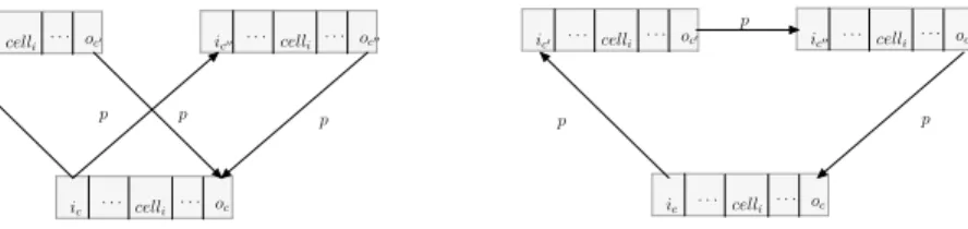
Figure 1 illustrates the functioning of rules of types (2) and (3). We denote by RM,x
the set containing all the rules defined above4. The above rules (where input and output positions are removed) simulate the run of a PSPACETM [12].
The following property formalizes the reduction and establishes its correctness.
ic . . . celli oc . . . ic0 . . . celli . . . oc0 ic00 cell oc00 i . . . . ic celli oc . . . . ic0 . . . celli . . . oc0 ic00 cell oc00 i . . . . p p p p p p p
Fig. 1. Existential (left) and universal (right) gadgets
Property 7. Let M be an alternating PSPACETuring machine, and let α be an atom of chase(IM,x,RM,x) representing a configuration c(α). Then c(α) is an accepting
configuration of M if and only if there is a path in chase(IM,x, RM,x) from i(α) to
o(α) whose label belongs to p∗.
Proof. (⇐) Let α ∈ chase(IM,x, RM,x) represent a configuration c(α), and let Cα
be the restriction of chase(IM,x, RM,x) to α. We show by induction on the number of
atoms of Cαthat the required path exists. Note that the induction is well-founded as the
Skolem chase is finite (recall that the considered Turing machines terminate).
– If Cαcontains one atom, then there can be no path in chase(IM,x, RM,x)
witness-ing p∗(i(α), o(α)). Suppose then that Cαcontains two atoms. In this case, the only
atom in Cαother than α must be p(i(α), o(α)). The only way to derive such an
atom is to apply a rule of the form (1), which is applied if and only if c(α) is in an accepting state, hence c(α) is an accepting configuration of M.
– Next assume that the result holds for any atom α such that Cαhas less than n atoms,
and let α be an atom such that Cαcontains n atoms. We distinguish two cases:
• Case 1: the state of c(α) is existential. Then, since the rules of type (2) must be satisfied, Cαcontains atoms α1and α2representing the successor
configu-rations of c(α). The existence of a path from i(α) to o(α) implies that there is either a path from i(α1) to o(α1) or a path from i(α2) to o(α2). To see why,
observe that every p-atom involving i(α) or o(α) is added either by the same rule application as created α or by a rule of type (2) applied to α. Only atoms of the second kind (refer to Fig. 1, left) can belong to a shortest path from i(α) to o(α), as atoms of the first kind have i(α) (resp. o(α)) as second (resp. first) ar-gument. If we have a path from i(α1) to o(α1), then we can apply the induction
assumption to α1to get that c(α1) is an accepting configuration, which implies
that c(α) is also accepting. We can proceed analogously if we have path from i(α2) to o(α2).
• Case 2: the state of c(α) is universal. As the rules of type (3) must be satisfied, the existence of a path from i(α) to o(α) implies the existence of a path from i(α1) to o(α1) and a path from i(α2) to o(α2), where α1 and α2 represent
the successor configurations of c(α) (refer to Fig. 1, right). By the induction assumption, c(α1) and c(α2) are both accepting configurations, which means
that c(α) is also accepting.
(⇒) We prove the other direction by induction on the number of transitions that need to be performed to prove that c(α) is accepted by M.
– If no transitions are required, this means that c(α) is in an accepting state. Thus, Rule (1) is applicable, and p(i(α), o(α)) is present in chase(IM,x, RM,x).
– Assume the result holds up to n required transitions. We distinguish two cases: • Case 1: the state of c(α) is existential. As c(α) is accepting, this means that one
of its two successor configurations, say c(α1), is accepting. Moreover, the
num-ber of transitions required to accept c(α1) is strictly smaller than for c(α). By
the induction assumption, p∗(i(α1), o(α1)) is present in chase(IM,x, RM,x).
As p(i(α), i(α1)) and p(o(α1), o(α)) are also present (since the rules of the
form (2) generate them), this proves that p∗(i(α), o(α)) is present as well. • Case 2: the state of c(α) is universal. As c(α) is accepting, this means that
its two successor configuration are also accepting. By the induction assump-tion, this means that p∗(i(α1), o(α1)) and p∗(i(α2), o(α2)) are present in
chase(IM,x, RM,x). As the rules of the form (3) also generate p(i(α), i(α1)),
p(o(α1), i(α2)), and p(o(α2), o(α)), this proves that p∗(i(α), o(α)) is present
in chase(IM,x, RM,x). ut
Now let M be an alternating PSPACE Turing machine, x be an input to M, and α be the unique atom in IM,x. Then by Property 7, c(α) is an accepting configuration
of M if and only if IM,x, RM,x |= p∗(i(α), o(α)). This, together with known results,
yields the following lower bounds:
Theorem 2. RPQ Answering in the presence of linear existential rules is NL-hard in data complexity,PTIME-hard in combined complexity with bounded arity andEXPTIME -hard in combined complexity without arity bound, even for a fixed RPQ.
Note that the preceding reduction can be easily adapted to show that atomic query answering under rulesets containing linear rules and transitivity rules is EXPTIME-hard. Assuming EXPTIME6=PSPACE, this result is in contradiction with Theorem 5 in [2], which purports to show a PSPACEupper bound. Indeed, after reexamining the proofs, the authors of the latter work have identified the flaw, which occurs in the analysis of the combined complexity of their rewriting-based decision procedure. It turns out that the procedure runs in exponential time, rather than in polynomial space (the NL upper bound in data complexity remains valid). Combining our lower bound with their procedure shows that the problem is EXPTIME-complete in combined complexity.
5
Conclusion and Future Work
In this paper, we have investigated the complexity of evaluating regular path queries un-der linear existential rules. We have shown that it is NL-complete in data complexity, PTIME-complete in combined complexity when the predicate arity is bounded, and EX
-PTIME-complete otherwise. This behavior is somewhat surprising with respect to prior work: indeed, for DL-LiteR, the combined complexity of RPQ answering is lower than
for CQs, whereas we observe just the opposite in the linear case (recall CQ answering is PSPACE-complete under linear rules). The upper bound was shown by adapting an existing decision procedure for DL-Lite, using a refined definition of type. The lower bound builds upon a PSPACE-hardness result for CQ answering under linear rules.
There are two natural ways to extend the present work: either investigate more ex-pressive forms of path queries (with conjunction and/or nesting) over linear rules, or consider the effect of moving to more expressive decidable classes of existential rules.
Acknowledgements. This work was supported by the ANR project 12 JS02 007 01.
References
1. Baget, J., Leclère, M., Mugnier, M., Salvat, E.: Extending decidable cases for rules with existential variables. In: Proc. of IJCAI. pp. 677–682 (2009)
2. Baget, J., Bienvenu, M., Mugnier, M., Rocher, S.: Combining existential rules and transitiv-ity: Next steps. In: Proc. of IJCAI. pp. 2720–2726 (2015)
3. Bienvenu, M., Calvanese, D., Ortiz, M., M.Šimkus: Nested regular path queries in descrip-tion logics. In: Proc. of KR (2014)
4. Bienvenu, M., Ortiz, M.: Ontology-mediated query answering with data-tractable description logics. In: Reasoning Web. pp. 218–307 (2015)
5. Bienvenu, M., Ortiz, M., Simkus, M.: Regular path queries in lightweight description logics: Complexity and algorithms. J. Artif. Intell. Res. (JAIR) 53, 315–374 (2015)
6. Bourhis, P., Krötzsch, M., Rudolph, S.: How to best nest regular path queries. In: Proc. of DL. pp. 404–415 (2014)
7. Calì, A., Gottlob, G., Kifer, M.: Taming the infinite chase: Query answering under expressive relational constraints. In: Proc. of KR. pp. 70–80 (2008)
8. Calvanese, D., Eiter, T., Ortiz, M.: Answering regular path queries in expressive description logics: An automata-theoretic approach. In: Proc. of AAAI. pp. 391–396 (2007)
9. Calvanese, D., Eiter, T., Ortiz, M.: Regular path queries in expressive description logics with nominals. In: Proc. of IJCAI. pp. 714–720 (2009)
10. Calvanese, D., Eiter, T., Ortiz, M.: Answering regular path queries in expressive description logics via alternating tree-automata. Inf. Comput. 237, 12–55 (2014)
11. Florescu, D., Levy, A., Suciu, D.: Query containment for conjunctive queries with regular expressions. In: Proc. of PODS (1998)
12. Gottlob, G., Papadimitriou, C.H.: On the complexity of single-rule datalog queries. Inf. Com-put. 183(1), 104–122 (2003)
13. Grau, B.C., Horrocks, I., Krötzsch, M., Kupke, C., Magka, D., Motik, B., Wang, Z.: Acyclic-ity notions for existential rules and their application to query answering in ontologies. J. Artif. Intell. Res. (JAIR) 47, 741–808 (2013)
14. Johnson, D.S., Klug, A.C.: Testing containment of conjunctive queries under functional and inclusion dependencies. J. Comput. Syst. Sci. 28(1), 167–189 (1984)
15. Kostylev, E.V., Reutter, J.L., Vrgoc, D.: XPath for DL ontologies. In: Proc. of AAAI (2015) 16. Maier, D., Mendelzon, A.O., Sagiv, Y.: Testing implications of data dependencies. ACM
Trans. Database Syst. 4(4), 455–469 (1979)
17. Marnette, B.: Generalized schema-mappings: from termination to tractability. In: Proc. of PODS. pp. 13–22 (2009)
18. Ortiz, M., Rudolph, S., Šimkus, M.: Query answering in the Horn fragments of the descrip-tion logics SHOIQ and SROIQ. In: Proc. of IJCAI (2011)
19. Stefanoni, G., Motik, B., Krötzsch, M., Rudolph, S.: The complexity of answering conjunc-tive and navigational queries over OWL 2 EL knowledge bases. J. of Art. Intell. Res. (JAIR) 51, 645–705 (2014)