HAL Id: hal-02978834
https://hal.archives-ouvertes.fr/hal-02978834
Submitted on 7 Nov 2020HAL is a multi-disciplinary open access archive for the deposit and dissemination of sci-entific research documents, whether they are pub-lished or not. The documents may come from teaching and research institutions in France or abroad, or from public or private research centers.
L’archive ouverte pluridisciplinaire HAL, est destinée au dépôt et à la diffusion de documents scientifiques de niveau recherche, publiés ou non, émanant des établissements d’enseignement et de recherche français ou étrangers, des laboratoires publics ou privés.
Design of a new electrical model of a ferromagnetic
planar inductor for its integration in a micro-converter
Rabia Melati, Azzedine Hamid, Thierry Lebey, Mokhtaria Derkaoui
To cite this version:
Rabia Melati, Azzedine Hamid, Thierry Lebey, Mokhtaria Derkaoui. Design of a new electrical model of a ferromagnetic planar inductor for its integration in a micro-converter. Mathematical and Com-puter Modelling, Elsevier, 2013, 57 (1-2), pp.200 - 227. �10.1016/j.mcm.2011.06.014�. �hal-02978834�
DESIGN OF A NEW ELECTRICAL MODEL OF A FERROMAGNETIC PLANAR
INDUCTOR FOR ITS INTEGRATION IN A MICRO CONVERTER
1
Melati Rabia, 2Hamid Azzedine, 3Thierry Lebey, 4Derkaoui Mokhtaria
Faculty of electrical Engineering - University of Science and Technology (USTO), Oran 31000
4
Université Paul Sabatier- Toulouse cedex 9 - France.
1
mel_ati@hotmail.fr, 2hamidazdean@yahoo.fr, 3thierry.lebey@laplace.univ-tlse.fr
Abstract
This paper presents a new electrical model of a ferromagnetic planar inductor with opposite entry and exit. Our aim is the monolithic integration of this type of inductor in a buck micro- converter.
Initially we choose the geometry of the planar spiral inductor which gives the highest inductance value; and by using the software FEMLAB3.1 we also simulate the electromagnetic effects in two types of inductors, one with a ferromagnetic core, and the other with- out, in order to choose the type of inductor which has better electromagnetic compatibility with the components of vicinity. A dimensioning of the geometrical parameters is carried out following a predimensioning.
By inspiring on the model of Yue and Yong, we design the new electrical model which highlights all parasitic effects generated by the core and the substrate, and allows calculation of the technological parameters. This model is much simpler than the model of Yamaguchi and takes into account some parasitic effects which were neglected by Yue and Yamaguchi.
To validate the results of dimensioning as well as the operation of the dimensioned inductor, we use PSIM6.0 software.
Keywords:
DC-DC Power converter, Integration, Ferromagnetic inductor, Geometrical parameters, Technological parameters, New electrical model1. Introduction
The power converters cover more and more scopes of application, This imply different environments of operation, starting from the domestic uses (general public), to the high applications to requirement for reliability (aeronautical); According to the application for which the converter is dedicated, one or more objectives of dimensioning are often specified and must be optimized.
The integration of various components of a static converter is actually the principal stake in the field of Power Electronics. Indeed, considering the development of distributed architectures or ―Systems-On-Chip‖, new technics must be developed to reduce size and reach better efficiencies. Even if much progress have been done in this field, some technological obstacles still prevent reaching powerful supply in a smaller place.
Planar spiral inductors are widely used in monolithic integrated circuits (MIC) for commercial wireless communications. However, these inductors often take up a large portion of the chip area, far more space than the active devices. In a typical amplifier MMIC (Monolithic Microwave Integrated Circuits) up to 80% of chip area is occupied by inductors. This is why the compact miniature inductors are highly desirable for low-cost, highly integrated MIC.
In integration, the choice of the topology and configuration of the inductor has a great importance, because it must make it possible to reach strongest possible values of inductance, with negligible losses on a minimal
section, and must have a good electromagnetic compatibility with the other components of vicinity. Its realization is also a parameter which must be taken into account.
The study of the literature on this subject, shows that spiral planar inductors are the most studied [1-10]; they are realized either on a magnetic core and a semiconductor substrate or only on a semiconductor substrate or between two layers of magnetic materials.
In the design of this type of passive components, for applications of power, the objective is to obtain an inductor having the following performances:
- High operating frequency (beyond the MHz), - Low resistances DC and AC,
- Low Compactness.
- A good electromagnetic compatibility with the close components.
The realization of a good compromise proves to be difficult, because the integration of such a component introduces additional disturbing elements compared to a regular coil, the substrate and the magnetic core; by their properties respectively semi-conductive and conductive, they cause additional losses of energies to high frequencies which will degrade not only the factor of quality, but also the operating frequency of inductor. The passive components concerned with this study are spiral planar ferromagnetic inductors that we will name ―Inductor MOFS‖ (Metal_ Oxide _ Ferrite _ Semi-conductor), and our aim is the monolithic integration of this type of component in a micro-converter.
This study does not relate to only the dimensioning of the geometrical parameters of the inductor, but takes into account the electromagnetic effects and the parasitic effects generated by stacking of various materials. To dimension the geometrical parameters with a minimum of energy losses, we use a new approach [11], and to calculate the technological parameters, we conceive a new electrical model of an inductor MOFS, this model highlight all the parasitic effects generated by the core, the substrate and the conductor.
By using software PSIM6.0, we visualize the waveforms of the currents and voltages in the micro-converter and at the boundaries of the integrated inductor, the form of these signals gives us a clear idea on the operation of the inductor and the micro-converter.
2. Possibilities of integration
Due to the increase in request, the research efforts in integration multiplied, and gave rise to several technologies. There exist today two integrations types of power: Monolithic integration and hybrid integration. Monolithic integration consists in realizing on the same substrate of the specific functions of power and of circuits or systems traditional which fulfill the functions of filtering (Figure 1), protection and even of order, and their interconnections.
In the hybrid approach, the component will result from the association of several functions in only one block, either by stacking, or by regrouping of functions (Figure 2), among the hybrid components, there exist the filters, the transformers, converters … etc. Whose advantages are: the reduction of the costs and dimensions, a simpler assembly…etc.
Fig.2: Principle and example of a converter developed by J.A. Ferreira.
3. Methodology of optimized design of integrated inductor
The dimensioning and the realization of an integrated inductor is a big step in the realization of a power converter. The optimization of the inductance value for a given surface will thus depend on several big factors. The dimensioning of an inductor, whatever the type of application for which it is intended, includes three stages:
_ Magnetic dimensioning, _ Electric dimensioning,
_ Mechanical and thermal dimensioning.
Magnetic dimensioning depends on the good choice of the magnetic material which makes it possible to store the quantity of wanted energy, of dimensions of the electrical circuit, and depends also of relative permeability and induction of saturation of the selected material.
A good magnetic dimensioning guarantees the obtaining value of the wished inductance, the limitation of the losses energy, and especially avoids saturation of the component.
Electrical dimensioning strongly depends on the geometrical parameters of inductor; its purpose is to minimize the losses by Joule effects in the conductor, and mitigate the capacitive, resistive and inductive effects which disturb the good performance of inductor.
The choice of the semi-conductor constituting the substrate is also a crucial factor in the optimization of a planar inductor, because it must not to be only compatible with the realization of the active circuits which compose the micro-converter, but it must also generate a minimum of energy losses.
4. Presentation of the micro converter
We choose a Buck micro-converter continuous-continuous step-down (Figure 3). The inductor that we want to integrate will thus be dimensioned for this type of application. We will choose the schedule of conditions according to:
Input Voltage: Vin5V
Cyclic report = 0.5
Output Voltage: Vout2,5V
Average output current : Isavg0,38A
Maximal current : IL max0, 6A
Operation frequency f1,5Mhz
Fig.3: Schematic diagram of the Buck converter.
The voltages and concerned currents are relatively weak. To increase the output of the micro converter, it is imperative to reduce to the maximum the energy losses inside this converter.
5. Needs and applications
The inductor that we wish to integrate falls under a general orientation tending towards the miniaturization and the total integration of the systems of small power. The applications concerned are the portable electronics, whose tendency always goes towards the reduction of the size and the number of components. Thus we will register this study in the field of the small power and more particularly that of the energy conversion.
Because of ease of its realization compared to other planar inductors, and the presence of experimental results cited in the literature, and thanks to its good electromagnetic compatibility, we focused our studies on the modelling of planar spiral inductor
.
6. Different geometries of planar spiral inductors
The planar spiral inductors are presented in different geometrical shapes, circular, square, octagonal, and hexagonal; they are all characterized by the same geometrical parameters: the number of turns n, the internal diameter din, the external diameter dout of inductor, the width w and the thickness t of the rectangular coil, and
the spacing inter-whorls s (Figure 4).
Before making our choice, we will study the influence of the geometry on the value of the inductance.
7. Choice of the geometry
We will choose now the geometry of the planar inductor that we wish to integrate. In the literature, we find several analytical expressions such as the formula of Bryan [12-13], the formula of wheeler [14] the formula of Mohan and al [15]… etc. These expressions enable us to make a comparison of the value of inductance for various spiral geometries: square, circular, hexagonal or octagonal.
7.1. Wheeler’s Formula
Wheeler’s expression allows an evaluation of the inductance of an hexagonal, octagonal or square reel carried out in a discrete way.
A simplification can be operated in the integrated planar case [14]. Inductance Lmw given by the method of Wheeler has as an expression (1):
2 avg mw 1 0 r 2 m
n d
L
k
1 k A
(1)Where "Am" is the factor of form, defined by expression (2):
out in m out in d d A d d . (2) And davg is the average diameter of coil winding defined by the internal diameter din , and the external
diameter dout by relation (3):
avg in out d d d 2 (3) 1
k and k2are two coefficients which depend on the used geometrical form . The values of these two coefficients are given in table1.
Table.1: Values of the coefficients used in formula of Wheeler.
Form k1 k2
Square 2,34 2,75
Hexagonal 2,33 3,82
Octagonal 2,25 3,55
We can consider in the Wheeler’s formula, that the value of inductance is proportional to ratiok k1 2 (Table 2). Table.2: Values of ratio
1 2
k k according to the geometry.
Geometry square hexagonal octagonal
Rapport 1 2
k k 0.85 0.82 0.63
The greatest value of ratio k k1 2is allotted to the square geometry
7.2. Monomial’s Formula
The expression of Monomial [16] used to calculate the inductance is based on the relation (4):
1 2 3 4 5
mon out avg
1 2 3 4 5
, , , , ,
: are Coefficients which depends on the geometrical form of the planar spiral inductor The values of these coefficients are given in Table3.
Table.3: Values of the coefficients used in formula of Monomial.
Geometry Square Hexagonal Octagonal
1,62 10-3 1,28 10-3 1,33 10-3 1 -1,21 -1,24 -1,21 2 -0,147 -0,174 -0,163 3 2,4 2,47 2,43 4 1,78 1,77 1,75 5 -0,03 -0,049 -0,049 1, 2 and 5
having negative values. We can consider that the value of the inductance is proportional to the
ratio
3 4
1 2 5
(Table 4).Table.4: Values of ratio
3 4
1 2 5
according to the geometry.Geometry Ratio
3 4
1 2 5
Square 1296,9472
Hexagonal 529,313
Octagonal 586,23
We also notice that the greatest value of ratio
3 4
1 2 5
is allotted to the square geometry.7.3. Mohan’s Formula
The expression given by Mohan for the calculation of inductance is expressed by relation (5) [15]:
2 0 avg 1 2 2 3 4 n d c c L ln c c 2 (5) Where ρ is the factor of form expressed by formula (6):
out in out in d d d d (6) 1 2 3 4
c , c , c , c are coefficients given according to the geometrical form (Table 5).
Table.5: Values of the coefficients used in formula of Mohan.
Geometry c1 c2 c3 c4
Square 1.27 2.07 0.18 0.13
Hexagonal 1.09 2.23 0 0.17
Octagonal 1.07 2.29 0 0.19
Circular 1 2.46 0 0.20
In Mohan’s formula, we consider that the value of inductance is proportional to the product
1 2 3 4
c ln(c ) c c .
Table. 6: Values of product
1 2 3 4
c ln(c ) c c According to the geometry.
Geometry Product c ln(c ) c1
2 3 c4
Square 1,299
Hexagonal 1,0594
Octagonal 1,0614
Circular 1,100
The four tables show that the square spiral geometry gives the greatest value of inductance, so will opt of a square spiral planar inductor.
8. Influence of the magnetic core in a planar inductor
A magnetic core in a planar inductor, not only allows to increase the value of inductance, to channel the magnetic flux, to store energy or to transmit it, but it also enables to decrease strongly the number of whorls, which mitigates the inter- whorls capacitive effect, as well as the capacitive effects due to the substrate and magnetic core; consequently it facilitates the realization of the inductor.
The choice of the used magnetic material determines the size of the component and confines the magnetic flux in the inductor, moreover containment of the lines of magnetic field is advantageous, because it attenuates the electromagnetic disturbances (EMI) of which the effects are accentuates with the increase of frequency; this causes an increase flow through the cross-section of the component (Figure 5) and notably an increase of the inductance value (by 10% to 100%) (Figure 6) for the same number of turns and the same occupied surface.
a) With magnetic layer
b) Without magnetic layer
Fig.5: Distribution of the magnetic flux of same intensity in a plan of transverse section of a planar spiral
with and without magnetic core.
102 104 106 108 0 0.5 1 1.5 2 2.5 3 3.5 4 4.5 5x 10 -6 Fréquence (Hz) In d u c ta n c e ( H )
L avec le noyau magnétique Lo sans le noyau magnétique
(a) (b)
Fig.6: Variation of inductance according to the frequency with and without magnetic core.
9. Simulation 3D of the different electromagnetic effects in a planar spiral inductor.
By using FEMLAB 3.1 software, we studied the electromagnetic compatibility of a planar inductor with the other micro converter’s components. Firstly we visualized the electromagnetic phenomenon in a planar inductor without (Figures 8 and 9) and with a magnetic core (Figures 11 and 12).
Fig.7: Planar inductor to be simulated without
magnetic core.
Fig.8: Propagation of magnetic field lines in a planar
inductor without magnetic core (front view).
Fig.9: Propagation of magnetic field lines in a planar inductor without magnetic core (view of profile).
Fig.10: Planar inductor to be simulated with a magnetic
core: front view.
Fig.11: Propagation of magnetic field lines in a planar
Fig.12: Propagation of magnetic field lines in a planar inductor with a magnetic core (front view).
We observe in Figures 8 and 9 the propagation of the magnetic field lines in all directions, that disturb the operating close components, while in Figures 11 and 12 , the majority of the magnetic field lines are concentrated at the walls of the magnetic block, there are only some lines which overflow of the other part of the spiral. Thus the electromagnetic disturbance with respect to the close components is very attenuated, but another problem emerges; we note the presence of a current which flows in the mgnetic core. this current is generated by capacitive effect and by the eddy currents (Figure13).
Fig.13: Eddy currents and displacement current in the core and substrate
induced by the flow of current in inductor.
To circumvent this problem we proceed as follows :
To attenuate the eddy currents; we cut out the magnetic core in plates according to our choice, vertically (Figure 14) or horizontally (Figure 15); and the currents due to the capacitive effects will be attenuated thanks to a good dimensioning of the electrical circuit and magnetic circuit of the inductor (it is the objective of our work).
It should be noted that the two directions of flaking do not present a difference from the magnetism point of view. On the other hand, we must choose the solution which facilitates the realization, and most adapted to planar technology.
We conclude finally, that to have a good electromagnetic compatibility of the inductor with the close components, it is preferable to insert a magnetic or ferromagnetic layer as an inductor's core.
10. Predimensioning of a planar inductor
Different geometrical parameters of inductor directly influence the inductance and resistance values, in the case of integrated inductor using planar technology: conductor’s width thickness, spacing, external and internal diameters, and number of turns.
Predimensioning in power electronics makes it possible to trim the design problem of the power converters. It especially makes it possible to ensure the functionality wished, as well as the respect of the principal specifications described in the schedule of conditions. So before carrying out a geometrical dimensioning, it is preferable to make a predimensioning.
10.1. Influence of the section of the conductor
For power applications, the conductor section (w.t) is an important factor, because it is this parameter which determines the mean levels of maxima current in front of being supported by the component. In addition, the study of the literature shows that if the conductor thickness has little influence on the value of inductance, it on the other hand will be determining on the value of resistance series. The reduction of the conductor’s width increases the value of inductance but at the price of an increase of the current density and consequently heating of the inductor. For this reason, the section of the conductor must be considered, firstly for the execution of a schedule of conditions; it is then fixed according to the maximum density of current tolerated by the structure. Once the section will be fixed, it remains to played only on the inter-whorls spacing ―s‖, and the number of turns ―n‖. To illustrate this study we choose a planar spiral inductor with an external diameter fixed at 900 µm and a frequency of operation equal to 1, 5 MHZ.
The skin effect is a phenomenon of electromagnetic origin, which exists for all conductors crossed by an alternative current and depends strongly on the frequency (Figure16): it causes the decrease of the current density while going far from periphery of the conductor to its center. It results an increase from the conductor’s resistance (Figure17); what leads to more important losses by Joule effect.
100 102 104 106 108 1010 0 0.5 1 1.5 2 2.5 3 Fréquence (Hz) R é si st a n c e ( o h m )
Fig.16: Variation of skin thickness according
to the frequency.
Fig. 17: Variation of resistance according
to the frequency. 0 2 4 6 8 10 x 106 0.2 0.4 0.6 0.8 1 1.2 1.4 1.6 1.8 2 2.2x 10 -4 Frequency (Hz) S ki n t h ickn e ss (m )
The skin thickness determines the width of the zone where the current concentrates in a conductor (Figure 18). The skin thickness is represented by relation ( 7):
f
(7)
With
μ μ μ
0 r (μ0 4π107H/m), µr is the relative permeability of material used as conductor.So that the current flows in the entire conductor, it is necessary that one of the following conditions be filled:
w 2 Or t 2 .
If the two conditions can be filled at the same time, it is the ideal, but in the case where only one condition
w 2 or t 2 can be realized; it is preferable to have the thickness "t" more important, or its width "w"?
Fig.18: Useful volume in a conductor delimited by the skin effect.
To slice, we will study the influence of the width ―w‖ (Figure 19) as well as the influence of the thickness ―t‖
(Figure 20) on the ratio R/L, with constant external and internal diameters.
Fig.19: Variation of ratio R/L for different values of the
width w.
Fig.20: Variation of ratio R/L for different values of the
thickness t.
The analysis of Figures 19 and 20 shows that the widening of the conductor as well as the increase of the conductor thickness, for a constant internal and external diameters, involve the reduction of the ratio R/L. but they cause a stressing of the capacitive effects.
10.2. Influence of the number of turns “n” and spacing “s”
For an occupied surface, fixed by the authorized maximum external diameter, the number of turns ―n‖ is finished. It remains to be seen if it is preferable to have an inductor with a strong rate of filling, or on the contrary to privilege a winding with few turns.
0 2 4 6 8 10 0 0.05 0.1 0.15 0.2 0.25 0.3 0.35 R a ti o R /L ( O h m .H -1 ) Number of turns w1=80µm w2=100µm w3=120µm 0 2 4 6 8 10 0 0.01 0.02 0.03 0.04 0.05 0.06 R a ti o R /L ( O h m .H -1 ) Number of turns t1=20µm t2=40µm t3=60µm
Figures 19 and 20 show that when the number of turns increases, for tending towards a maximum filling, the ratio R/L decreases, but, an important number of turns in a planar inductor, accentuates capacitive effects, as the inter-turns capacitive effect whose influence appears when the operating frequency increases.
It should be noted that figures 19 and 20 are traced for fixed internal and external diameters, therefore if the conductor width "w" increases, implies automatically decreasing of spacing inter-whorls ―s‖, and also decreasing of ratio R/L. But a narrow spacing between the turns is also in favour of the accentuation of parasitic effects. .
For this geometrical study, it emerges that:
The maximum surface that must occupy a planar spiral inductor is determined by the volume of the substrate (or of the magnetic core in the case of a ferromagnetic inductor), the determination of a set of geometrical parameters suitable ensuring the lowest ratio R/L, must answer several rules. By studying the variations of the ratio R /L, according to the various geometrical parameters, several conclusions arise in order to establish a methodology of predimensioning.
Thus, it is first of all necessary to translate the constraints imposed by a given current fixing in a final way the
section of the conductor ―w.t‖. In the same way, minimum ratio R/L can be reached by decreasing spacing
―s‖ as much as possible, while making sure that the rate of filling of the spiral is maximum; but a narrow
spacing accentuates the capacitive effect inter-turns which degrades the performances of the inductor. To circumvent this problem, we choose the condition t 2 instead of w 2 , because by decreasing the thickness ―t‖ we mitigate the inter-turns capacitive effect.
From this geometrical study, we will dimension a square planar spiral inductor for its integration in a micro- converter.
This inductor is made up of a copper winding, a magnetic core which is an alloy of 20% of iron and 80% of nickel (N fi e) and a semi-conductor substrate of silicon.
11. Dimensioning of the inductor
The steps for the design of planar spiral inductor are represented by the following algorithm (Figure21).
11.1. Dimensioning of the magnetic circuit
From schedule of conditions, we define the specifications of the micro converter which constitutes the starting point for the dimensioning of the inductor. By taking into account of selected electric and magnetic characteristics, we evaluate the volume of the magnetic core, which enables us to define the section on which we will put the electrical circuit of the inductor; then we will evaluate the dimensions of this circuit allowing to answer the specifications of the converter in terms of magnetic storage of energy and losses in materials. The following equations enable us to calculate the value of the necessary inductance for the realization of the micro converter; the voltage across the inductor depends on the variation of current flowing in this latter (Equation 8). L e dI V L dt (8) During the state on, the current which flows through the reel increases according to relation (9):
At the end of the state on, the current IL increased:
on L max Lm in
I I I
(9) The operating process is imposed by the average output current Isavg .
savg Lavg Cavg
I I I
(10)
Cavg
I 0A
since the average current in the condenser is null in permanent mode, thus: isavg iLavg
L max L min
Lavg L min savg L max
I I I I 2I I 2 (11) L min
I 0,16A,Ion0, 44A and IL max 0, 6A
Thus the micro converter functions in mode of continuous conduction, i.e. that the current in the reel is always positive and never cancels itself (Figure 22).
Fig.22: Evolution of the voltages and currents with time in an ideal buck converter
operating in continuous mode.
Duration of the period T during which the switch M1 is closed (Figure 3), leads to an increase in energy stored in the inductor, this duration represents the cyclic ratio α; for a step-down we have:
out in
V
0,5
V
(12)e on V (1 ) I L f (13) The undulation of currentIonis maximum for 0, 5. Knowing the values of the frequency, input voltage
and undulation of currentf1,5 MHz, Vin 5Vand Ion0, 44A, we can calculate the value of the
inductance L: e on V (1 ) L 1,89 H I f (14)
Thus we must carry out a micro reel whose value of inductance will be 1,89µH, this value makes it possible to determine the stored energy and consequently the volume of magnetic circuit, which enables us to evaluate the external diameter of inductor; The diameter being fixed, we can calculate the other geometrical parameters (Figure4) which are: the number of turns ―n‖, the internal diameter ―din‖ of inductor , the width ―w‖ and the thickness ―t‖ of the rectangular coil, and the spacing inter-turns ―s‖. Evaluation of these parameters is the subject of our study.
An insulator is placed between the core and the conductor on the same level in order, to isolate the electrical circuit from the magnetic circuit of the inductor.
11.1.1. Calculation of the volume of the core
The value of inductance being given; it is possible to calculate the maximum energy to be stored in this component by relation (15) 2 max LI 2 1 W (15) For an inductance of 1,89µH, crossed by a maximum current of 0,6 A, the inductor can store 0,34 µj.
To determine the volume of ferrite necessary to this stocking, we must know the voluminous density of energy characterizing this material. This density is given by equation (16)
2 max v max 0 r B W 2 (16) The necessary volume to store energy will be fixed by the maximum magnetic induction Bmax which can support the material, and its relative permeability µr. 0is the magnetic permeability of the free space
( 7 1
0 4 10 Hm
). In the case of an alloy Ni-Fe (80% of nickel and of iron 20%) and without air-gap whose
characteristics are: r 800 and Bmax 0, 6 T, we obtain: 3
v max
W 179Jm . The volume of the ferromagnetic
core is given by relation 17.
9 3 v max W Vol 1,9.10 m W (17)
1, 9 mm3 of Ni-Fe is necessary to store 0, 34 µj.
Let us note here that more the magnetic permeability will be raised, more the volume of the magnetic circuit will be important, for a given maximum induction.
12. Dimensioning of the electrical circuit of inductor
The volume of the ferromagnetic core being evaluated to 1,9 mm3 , We will make a game of dimensions, we
consider the core as a block having a thickness of 1,6 mm, what gives a square section equal to 1,1875 mm2
that we name Amag it is the section on which we will put the spiral coil, each of its sides is equal to 1,089 mm; if we leave on each side a distance of 95 µm, the external diameter will of the inductor be equal to 900 µm.
The calculation of the values of other geometrical parameters of the electrical circuit is based on quite precise conditions.
12.1. Calculation of the number of turns
We find in the literature several formulas which allow us to calculate the number of turns according to the value of inductance, such as the formula of Bryan, the formula of wheeler, the formula of Mohan and formula of Monomial. If we calculate the number of turns with the three formulas, the results will be almost identical. So we are forced to choose one method. We chose the method of Wheeler; it allows an evaluation of the inductance of an hexagonal, octagonal, square reel, carried out in a discrete way. A simplification can be operated in the integrated planar case [14]. Inductance given Lmw by the method of Wheeler has as an expression (18): 2 avg mw 1 0 r 2 m
n d
L
k
1 k A
(18)The coefficients k1 and k2 are defined for each geometry, for a spiral square, k12,34 and k22,75
.
While putting: in out d c d we obtain formula (19):
2
2 0 r 1 ou t 2L (1 c) k (1 c) n k d (1 c) (19)We choose as report c0, 25
,
so with the external diameter dout900 m,
the internal diameter will be ind 225 m and we obtain a number of turns: n 1,95 2
.
12.2. Calculation of the thickness “t” and the width “w" of the conductor
The calculation of these two parameters depends on the skin thickness.
To circumvent this problem, let us calculate the width ―w‖ and the thickness ―t‖ of the conductor according to the skin thickness, and to the surface density of current which flows in this last. For a rectangular conductor, the formulas are as follows [18]:
x ix 0 j(x) j e e , and x 0 j(x) j e (20) With f
The average value of the surface current density is:
t 2 0 avg j e 1 j 2 (21) For copper 8 1,7.10 m and r 1we have 0 r, 7 1 0 4 10 Hm , and frequency f 1,5 MHz we will obtain after calculation 53,57µm
So that the current flows in the entire conductor, it is necessary that one of the following conditions is carried out: w 2 or t 2 .
We impose one of the two values ―t‖ or ―w‖; from the predimensioning it is preferable to give the smallest
value to the thickness ―t‖. In putting t 50 m we can calculate the width ―w‖. In order that a maximum current I0,6A can flow in the coil conductor, it is necessary that the section S of this conductor meets the conditions (22):
avg
IS j with Sw.t (22)
It should be noted that the acceptable current density in a planar inductor is higher than that in the large reels, because the losses by Joule effect which overheat the conductor are proportional to its volume. In the majority of cases, micro-conductors are in contact with substrates having good properties of temperature conduction.
According to dimensions and the form, the densities of current from 3
10 to 104 (A / mm )2 are then possible.
What enables us to put as conditions to boundaries: 3
2
9
2
0
j 10 Amm 10 Am .
After calculation, the average current density and the section of the rectangular conductor are estimated at:
9 2
avg
j 0,313.10 Am and S 1914,79 m 2
.
1914,76 m2 represents the minimal conductor’s section which makes flow a maximum current of 0.6 A with an average current density of 0.313.109 Am-2, which gives a minimal width w=38,29m
.
Since theconditiont 2 is respected. We can increase the value of w. We thus put a width w= 130m
.
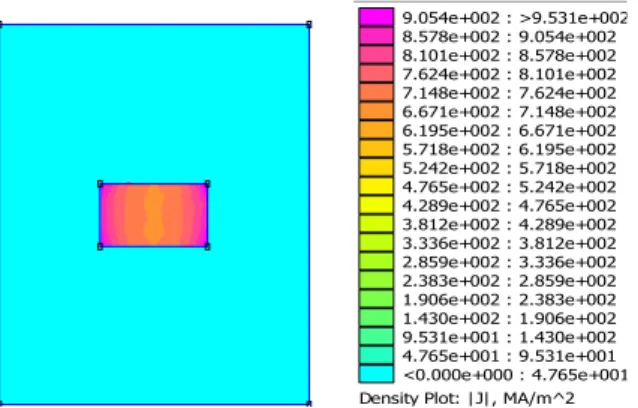
12.2.1. Simulation of the section of the conductor.
By using software FEMM 4.2, we simulate the dimensioned conductor of the inductors, in order to ensure us that the skin effect is completely circumventing; the result is given by figure 23.
Density Plot: |J|, MA/m^2 9.054e+002 : >9.531e+002 8.578e+002 : 9.054e+002 8.101e+002 : 8.578e+002 7.624e+002 : 8.101e+002 7.148e+002 : 7.624e+002 6.671e+002 : 7.148e+002 6.195e+002 : 6.671e+002 5.718e+002 : 6.195e+002 5.242e+002 : 5.718e+002 4.765e+002 : 5.242e+002 4.289e+002 : 4.765e+002 3.812e+002 : 4.289e+002 3.336e+002 : 3.812e+002 2.859e+002 : 3.336e+002 2.383e+002 : 2.859e+002 1.906e+002 : 2.383e+002 1.430e+002 : 1.906e+002 9.531e+001 : 1.430e+002 4.765e+001 : 9.531e+001 <0.000e+000 : 4.765e+001 Density Plot: |J|, MA/m^2
9.054e+002 : >9.531e+002 8.578e+002 : 9.054e+002 8.101e+002 : 8.578e+002 7.624e+002 : 8.101e+002 7.148e+002 : 7.624e+002 6.671e+002 : 7.148e+002 6.195e+002 : 6.671e+002 5.718e+002 : 6.195e+002 5.242e+002 : 5.718e+002 4.765e+002 : 5.242e+002 4.289e+002 : 4.765e+002 3.812e+002 : 4.289e+002 3.336e+002 : 3.812e+002 2.859e+002 : 3.336e+002 2.383e+002 : 2.859e+002 1.906e+002 : 2.383e+002 1.430e+002 : 1.906e+002 9.531e+001 : 1.430e+002 4.765e+001 : 9.531e+001 <0.000e+000 : 4.765e+001
Fig. 23: Representation of the conductor after circumventing of skin effect.
The dimensioning of the conductor's section gives an encouraging result, because Figure 23 shows that at a frequency of 1.5MHZ, this section is completely crossed by the current, and there is not any deserted part, therefore the problem of increase in resistance series and heating of the ribbon conductor is eliminated.
12.3. Calculation of inter-turns spacing
From the geometry of the square inductor, we establish formula (23):
out in out in d d 2wn d d 2wn 2s(n 1) s 2(n 1) (23)
12.4. Calculation of the average conductor length.
The average length of the coil conductor in a square spiral inductor is deduced from the expression (22):
avg out
l 4n d (n 1)s nw s (24)
12.5. Results of dimensioning of electrical circuit
The essential parameters of planar inductor that we want to integrate are gathered in the table 7.
Table 7 shows that the computed values of the geometrical parameters are in the standards of integration, thus the result of dimensioning is encouraging.
13. Modeling of a spiral planar inductor
13.1. Planar inductor without magnetic core
After Nguyen and Meyer in 1990 [19-20] which were the first with proposed a simple model in ―π‖ to describe the behaviour of a planar inductor integrated on silicon. An improved model was developed later by Ashby and Al [20-21]. However the parameters of the model need to be adjusted starting from the experimental curves, rather than to have a physical significance. More recently Yue and Yong [22] brought back a similar model (Figure 25) but with parameters more appropriate to the geometry of inductor. The electric diagram of a spiral planar inductor is deduced starting from its transverse section (Figure24).
Fig.24: Transverse section of a spiral planar
inductor.
Fig.25: Model in ―π‖ of a spiral planar inductor developed by Yue
and Yong [22].
13.2. Planar inductor with magnetic core
When a magnetic metal layer is built above (or below) of the inductor, the model becomes considerably complicated because of the interactions between layers stacking (Coil - Magnetic core - Substrate) constituting the inductor. The first equivalent diagram (Figure 26) was proposed by Yamaguchi and al [23].
Table. 7: Results of the dimensioning of geometrical parameters
Geometrical parameters Results of dimensioning
Number of turns: n 2
Average length: lavg 4,418 mm
Width: w 130 µm
Thickness: t 50 µm
Spacing inter-turns: s 78 µm
External diameter : dout 900 µm
Fig.26: Model in ―π‖ of a ferromagnetic planar inductor [23].
This model takes into account the parasitic capacities CSm1 and CSm2 between the magnetic layer and the
inductor which are due to the potential differences between the coil and the magnetic layer. Such capacities Cpm1 and Cpm2 also exist between the magnetic plan (potential floating) and the substrate (potential with the
mass). These capacities are associated with resistances Rpm1 and Rpm2 which correspond to the losses associated
by Joule effect in silicon. Another Cmag capacity is also added in series with the main inductance (Lmag) if the
magnetic material is split into separate components, this corresponds then to the capacity of these magnetic elements. This Lmag inductance corresponds to the fraction of inductance (LS) increased by the presence of the
magnetic layer with strong permeability. It is also accompanied by a series resistance type Rmag which takes
into account the Joule effects in the magnetic layer and the losses in Lm inductance due to the presence of this
conducting magnetic layer.
14. New electrical model of a ferromagnetic inductor
In a physical model each circuit element is related directly to the physical layout. This property is very important when designing new inductors or transformers where measurements data are not available. The key to accurate physical modeling in this way is the ability to describe the behaviour of the inductance and the parasitic effects. Each lumped element of the model should be consistent with the physical phenomena occurring in the part of structure it represents. In a pure physical model the value of electrical lumped elements is only determined by the geometry and material constants of the structure.
During modeling, we have to be prudent about the accuracy and limitations of the model.
Inspired by the model of Yu and Yong, we design a new electrical model of a spiral planar inductor with a ferromagnetic core and a silicon substrate. The aim of this new model is to minimise the number of components in the equivalent circuit. The basic idea is to model the whole winding as one lumped physical element with two ports. Accordingly, the inductance and all parasitics just relate to one physical element. The Figure 28 shows the equivalent circuit resulting from the transverse section (Figure 27). It represents an almost symmetrical pi-circuit with ports on both sides. We gave to this type of inductance the name MOFS ―Metal-Oxide-Ferrite-Semi-conductor‖.
Fig.28: New Model of a ferromagnetic inductor ―MOFS‖. 14.1. Discussion and interpretation
If we manage to integrate a planar inductor in an electronic device, this inductor must have two connections, one at its entry and an other at its exit. In literature, the exit of the spiral is carried out through a conductor buried in the insulator which is placed at the lower part of winding. Neither the model of Yue, nor the model of Yamaguchi took into account the parasitic effects which generates the buried conductor. In this work, we present a new electrical model of planar spiral ferromagnetic inductor in which entry and exit are opposites (Figure 32). The electrical model corresponding at a ferromagnetic spiral planar inductror where the entry and the exit are on the same side is in reference [11].
Fig.29: Planar inductor of which entry and the exit are in the same direction
(a) Front view, (b) View of profile.
Fig.30: Planar inductor with opposite entry and exit
14.2. New electrical model of ferromagnetic planar inductor with opposite entry and exit
Starting from the transverse section of the ferromagnetic spiral planar inductor (Figure 31), we posed the corresponding electrical model with opposite entry and exit (Figure 32).
Fig.31: Transverse section of the ferromagnetic spiral planar inductor ―MOFS‖
with opposite entry and exit.
Fig.32: New Model of an inductor ―MOFS‖ with opposite entry and exit
15. Calculation of Technological parameters
Before passing to the realization of an inductor following a dimensioning such as that described above, new elements must be taken into consideration in order to determine if the beforehand fixed geometrical parameters will induce a correct frequential behavior of the component. For that, we must be interested in other parasitic elements, which are mentioned in Figure 32.
First of all, by construction a planar inductor has an inter-turns capacity Cs expressed by relation (25); whose
influence appears when the use frequency of the component increases.
avg s 0
t l
C
s
(25) ε0 is the permittivity of free space.The series resistance of the winding conductor is also a crucial problem in the design of inductors. Moreover, when inductor works at dynamic mode, the metal line suffers from skin effects and proximity effects, and series resistance R becomes function of the frequency. s
avg avg s l l R S w t (26) When w 2 and t 2 , Rs will be expressed by relation (27) :
avg s eff l R w t (27) Where teff is function of the conductor thickness ―t― and the skin thickness ―δ‖:
t / eff
t (1 e ),
ρ is the resistivity of the cooper 8
copper 1,7.10 m
.
The inductor which we wish to integrate being of type MOFS, an oxide is essential to ensure an electrical insulation between the electrical circuit and the ferrite, which is in its turn put on a semi-conductor substrate. This piled structure generates various parasitic elements which imply increasingly important losses of energy when the frequency increases. The study of the literature provides several expressions allowing the calculation of some of these parasitic elements. In this regard, the most cited reference work is those of Yue [22].
The substrate and ferrite resistances Rsub and Rmag represent respectively the ohmic losses in the substrate
and the core (ferrite). They are caused by the current flowing between the winding conductor and the ground contact. Although the winding is put on a non-conducting dielectric, a current flows through the capacitive coupling between winding and substrate, and between the ferrite and ground contact. An appropriate expression for the substrate resistance is derived from reference [24].
The substrate resistance calculation is based on the area where the capacitive coupling acts on the substrate. This area depends on the width ―w‖ and the average length ―lavg‖of the winding. These parasitic effects
degrade the performances of inductor.
The succession Metal-Oxide-Semi-conductor creates an oxide capacity C , in the same way the substrate ox
material block between two ideal conductor plates, is represented by an electrical equivalent circuit of a physical configuration which consists of the resistance Rsub and the shunt-capacitor Csub in parallel.
If the internal port of inductor is brought back towards outside by a buried contact, the potential difference between the whorls and the buried conductor can induce stray capacities. We also consider that the capacity
v1
C is equivalent to the sum of the capacities of covering between the buried conductor and the different whorls, capacity Cv 2is between the buried conductor ant the core (Figure 31).
The circuit in “π” being symmetrical (without capacities C and v1 Cv 2), we have:
ox ox1 ox 2 C C C 2 (28) sub sub1 sub2 C C C 2 (29)
sub1 sub2 sub
R R 2R (30)
mag1 mag2 mag
R R 2R (31) We model usually the capacities in an integrated inductor starting from the concept of capacity with parallel plates: ox1 0 ox ox 1 A C 2 t (32)
sub1 0 si sub 1 A C 2 h (33) avg s 0 t l C s (34)
2 v1 0 ox 1 2 n 1 w C t (35) v2 0 ox 2 3 [nw (n 1)s d]w C t (36)It should be noted that the width of the buried conductor is equal to the width ―w‖. The suitable expressions for the substrate and ferrite resistances are given by relations (37) and (38):
sub sub1 Si h R 2 A (37) mag mag1 NiFe h R 2 A (38)
The resistance of the buried portion of the conductor ribbon is expressed as follows:
b [nw (n 1)s d] Rb w h (39) Where hsub, hmag, tox and h represent respectively thickness of substrate Si ,ferrite Nb iFe, the oxide of silicon
SiO2 ,and the buried conductor of copper; 1 2
t and t2 3 are respectively distances between the spiral and the buried conductor, and between the buried
conductor and the ferrite, A represent the conductor section which is in contact with insulator (Alavg.w) and
d is the distance left from each side on the section Amag.
si 18,5 m
and 8
NiFe 20.10 m
are the respective resistivities of silicon and ferrite NiFe,
1 0
( 8,85 pF.m ) ,
si 11,8
and ( ox 3,9) are the respective relative permittivities of free space, of the silicon and of the oxide, ―lavg‖ represents the average length of the coil , ―w‖ its width, ―n‖ is the number ofturns.
mag
h =1,6 mm. In puting hsub= 50 µm,
t1-2= t2-3=20µm tox= 60 µm , hb=20µm, and d=95µm The results are grouped in Table 8.
Table.8: Results of technological parameters of a ―MOFS‖ inductor with opposite entry and exit.
Technological parameters Calculated values
Cs (pF) 0,025 Cox1 (pF) 0,17 Csub1 (pF) 0,6 Cv1 (pF) 0,03 pF Cv2 (pF) 0,097 PF Rs(Ω) 0,017 Rb(Ω) 113.10-5 Rmg1(MΩ) 56.10-5 Rsub1(KΩ) 2,05.10-3
The following Table 9 gives the results of technological parameters of the ―MOFS‖ inductor where the entry and the exit are on the same direction [ 20].
It is noted that the values of these parameters are calculated with the same schedule of conditions as the precedent Table 8.
Table.9. Results of technological parameters of an inductor ―MOFS‖ with entry and exit at the same direction.
Technological parameters Calculated values Cs (pF) 0,025 Cox1 (pF) 0,17 Csub1 (pF) 0,6 Cv1 (pF) 0,056 Cv2 (pF) 0,17 Rs(Ω) 0,017 Rb(Ω) 205.10-5 Rmg1(MΩ) 56.10-5 Rsub1(KΩ) 2,05.10-3
16. Interpretation of results
The aim of this work is to minimize the losses of energy in the inductor, i.e. to mitigate the capacitive and resistive effects due to the induced currents and the eddy currents; for that, the values of the capacitances C , ox
sub
C , C and v1 C must be as weak as possible, to avoid all infiltrations of currents in the substrate and in the v2
magnetic core; on the other hand the values of resistances Rmag and Rsub must be as high as possible to avoid
the passage of the currents induced by capacitive effect in the substrate and the core; but resistances Rb and s
R must be very low to facilitate the flow of current in the conducting ribbon.
The computed values of the technological parameters which strongly depend on the geometrical parameters are in agreement with the wished objectives.
The values of resistances R and s R are negligible, the values of the capacities b C , ox Csub, C and v1 C are v2 very weak; on the other hand the resistance Rmag is too low, therefore it facilitates the infiltration of the induced current towards the substrate, but the resistance Rsub is sufficiently strong to make barrier with this
current.
17. Simulation of the electrical circuit of the integrated inductor
To test the results of the dimensioning of the planar spiral ferromagnetic inductor, we use the PSIM6.0 software.
To validate the results of our work, we simulate with software PSIM6.0 the equivalent electrical circuit of the micro-converter containing the electrical circuit of the dimensioned square spiral planar inductance. This simulation is carried out using the results of Tables 8 and 9, and values of micro-converter capacitance and a load resistance.
This simulation enables us to make sure that the values allotted to the geometrical and technological parameters after dimensioning do not disturb the operation of the inductor. And also allows us to see that the integration of this inductance in the micro-converter ensures a good performance of this last.
At the first time, we simulate the electrical circuit of a micro-converter containing an ideal inductor without any parasitic effects, to be sure of the good operating micro-converter (Figures 34 and 35).
At the second time, we simulate the electrical circuit of a micro-converter containing a dimensioned ―MOFS‖ inductor with all its parasitic effects,once, the ―MOFS‖ inductor with entry and exit on the same direction (Figures 36 and 37); and another once the ―MOFS‖ inductor in with opposite entry and exit (Figures 38 and 39).
After visualization of the waveforms of currents and voltages in the micro-converter, we record at two diffrent moments , the minimal and maximum values of these latters.
The comparison of the waveforms of voltages and currents, resulting from the three simulations, as well as their measered values , will be carried out thereafter.
To simulate the electrical circuit of the micro-converter, we must calculate the value of the capacitance as well as the value of the load resistance.
17.1. calculation of the value capacitance of the micro-converter
We want a constant voltage at the exit of the micro-converter , but in practice this is not the case.
The output current Is being almost constant, the great variation of the inductor current IL can be absorbed only
by thecondenser.
The current flowing in the condenser (Ic= IL-Isavg) is a triangular current, The voltage Vc on its terminal
is thus made up of parabola arcs (figure33) .
out
1
Vc V Idt
C
(40) At the moment 1 ( Figure 33) the voltage is minimal, it goes up then and reaches its maximum when the totalsufrace marked in red is added (Moment 3). The undulation amplitude is the surface of this triangle that is to say (0,5x base x Height).
out out 2 in V 1 1 T I 1 ( ) V 1 C 2 2 2 8Lf C V (41) Where out out in 2 out V V 1 V C 8Lf V (42) The capacitance value is inversely proportional to the undulation of the output voltage; thus we can exploit the value of capacitance C to attenuate this undulation and to have a more or less constant output signal.
By choosing an undulation of the output voltage of about 5% of the average value of Vout, we obtain a value of capacitance: C=0,29µF.
R being the output load, we have:
out savg
R= V /I ; R= 6,57 Ω
17.2. Simulation of a micro-converter circuit with an ideal inductor.
Fig.34: Micro-converter circuit with an ideal reel.
Fig.35: Waveforms of the currents and voltages of a micro-converter containing an ideal reel. Table.10: Maximum and minimum values of voltages and currents
Time (s) 1.97793e−5 2.01404e−5
VL −9.97817e−1 1.83677e+0 IL 4.85022e−1 3.86323e−1 VC 2.59393e+0 2.40003e+0 IC 5.27001e−2 −1.36812e−2 VS 2.59393e+0 2.40003e+0 IS 4.32322e−1 4.00004e−1
The waveforms of Figure 35 reflect those of a Buck converter , the current at the boundaries of the reel is corrugated and never itself cancels, therefore the continuous conduction mode is respected; the terminals voltage of the capacitor and the output voltage are similar and continuous, with a light undulation. We also notice a continuous output current, and a transitory mode during the first micro seconds.
17.3. Simulation of a micro-converter circuit with a MOFS inductor with entry and exit at the same direction.
Fig.36: Micro-converter circuit with a dimensioned MOFS inductor with entry and exit at the same side.
Fig.37: Waveforms of the currents and voltages of a micro-converter containing MOFS inductor
Table.11. Maximum and minimum measured values of voltages and currents
Time (s) 2.01003e−5 1.98195e−5
VL 6.55253e−1 −2.42465e+0 IL 2.70421e−1 3.83511e−1 VC 2.14187e+0 2.26420e+0 IC −8.65580e−2 6.14400e−3 VS 2.14187e+0 2.26420e+0 IS 3.56979e−1 3.77367e−1
The waveforms of figure 37 are also similar to those of a Buck converter; we must now check if the dimensioning of the inductor is perfect or not, for that, we will draw up a summary table which contains results of three simulations, then we compare the results of the two last with those of the first.
17.4. Simulation of a micro-converter circuit with a MOFS inductor with opposite entry and exit
Fig.38: Micro-converter circuit cwith a dimensioned MOFS inductor with opposites entry and exit.
with opposites entry and exit.
Table.12. Maximum and minimum measured values of voltages and currents. Time (s) 1.98195e−5 2.01404e−5
VL −2.42540e+0 2.00926e+0 IL 3.83657e−1 3.31348e−1 VC 2.26495e+0 2.13595e+0 IC 6.16592e−3 −2.46442e−2 VS 2.26495e+0 2.13595e+0 IS 3.77491e−1 3.55993e−1
We notice in figure 39 that the waveforms are respected and reflect those of a Buck converter, we thus conclude that if we change the exit of the inductor in order to have entry and the exit in opposed directions, the operation of the latter will not be disturbed. We conclude finaly that the proposed new electrical circuit of a ferromagnetic inductor with opposite entry and exit functions perfectly.
17.5. Interpretation of results.
The table 13 gathers the results of the three simulations.
Table.13: Table of results comparison of a three simulations. T.I
C.V I.I I.OEE I. EESD SV
ILmax 0,48502 0.38365 0.38351 0.6 ∆IL 0.09869 0.05231 0.11309 0.16 Isavg 0,41616 0.36674 0.36717 0.38 ∆Is 0.03231 0.02149 0.02039 / Vs.avg 2.49698 2.2005 2.20303 2.5 ∆Vs 0.09695 0.129 0.12235 0.125
T.I: Type of Inductor C.V: Current and Voltage I.I: Ideal Inductor
I.OEE: Inductor with Opposite Entry and Exit
I. EESD: Inductor with Entry and Exit at the Same Direction.
To interpret the results of these simulations, we calculate the relative errors of the voltages and the output currents (Table 14).
. Table.14: Relative errors of currents and voltages.
R.E: Relative Error.
T.I
R.E
T.I I.I I.OEE I.SEE S.V
Is Is 7.76℅ 5.85℅ 5.55℅ 5℅ Vs Vs 3.88℅ 5.86℅ 5.55℅ 5℅
The average value of the output current in the inductor in which entry and the exit are at the same direction is very close to the desired value: 0.36717 A instead of 0.38 A, with a relative error of 5.55℅. The inductor in which entry and exit are opposed, comes in the second place with the same relative error and an average value of the output current from 0.36674 A instead of 0.38 A. while the ideal inductor presents a relative error of 7,76℅, and an average value of the output current slightly higher than the desired value.
If we take into account the voltages, the ideal inductor has the best results with an output voltage (we can say) equal to the wished output voltage , and an undulation relative error of 3,88 ℅ better than the desired relative error.
The two integrated inductors also present an output voltage, close to the desired value, 2.2005 V for the inductor with opposite entry and exit and 2.20303 V for the inductance in which entry and the exit are the samedirection, instead of 2.5V which is the desired value.
The undulation relative error is slightly larger than the desired error 5,5℅ instead of 5℅.
In conclution we can say that the new electrical circuit of an integrated ferromagnetic inductor with opposite entry and exit, that we conceived, respects the waves form currents and voltages, exactly like that of an ideal reel . It is a encouraging point.
Concerning the dimensioning of the ferromagnetic inductor, the results are very encouraging, because the average values of the tensions and currents at the output of the micro-converter, are very close to the desired values. but we can have better results.
To adjust the average value of the output current Iavg, we can exploit the value of the load resistance , while
respecting the continuous conduction mode.
To attenuate the undulations of the output voltage Vout, we can exploit the value of the capacity of the micro-converter, while respecting the integration values for a condenser.
And finally, to have more exact value of the output voltage, we can play on dimensions of the conductor width and of the spacing inter-whorls, so to mitigate to the maximum the capacitive and resistive effects in the ferromagnetic core, and substrate.
18. Comparison and Interpretation
The study of the literature about the losses of energies in a planar inductor enabled us to define the causes of these losses and to establish relations with the component geometry;
To circumvent this problem, we proposed a new approach as well as a new electrical model of a spiral planar inductor with a ferromagnetic core and a semiconductor substrate which enable us to dimension the inductor and mitigate all parasitic effects. This dimensioning is carried out by taking account of the acceptable current by inductor and of the electromagnetic characteristics of used materials.
Several papers in literature treat the problem of dimensioning of planar inductors, but the majority of these papers are based on a set of dimensions.
For example, the dimensioning suggested by Alain Salles rests on a successive research of the value of inductance and resistance by modification of a set of geometrical parameters.
He regards as set of dimensions, the external diameter of inductor (3000µm), the conductor width (15µm), the spacing inter whorls (1µm) and the conductor thickness (15µm).
By studying the variations of the inductance and the series resistance of the inductor according to its geometrical parameters (n, w, t and s); Alain presents his methodology of dimensioning. By using those parameters, he determines the optimal performances of an inductor; but various iterative calculations are then necessary .
The dimensioning of the technological parameters which are due to the parasitic effects generated by the core and the substrate was neglected. We can also say that the model presented by Allain Salles is limited because it provides the values of inductance and resistance only in low frequencies
Troussier also treats the problem of dimensioning of a planar inductor, but it carries out only the dimensioning of the core and neglects completely the dimensioning of the spiral, although the geometrical parameters of the
conductor play a crucial role in attenuation of the parasitic effects due to stacking of different materials of inductor.
Troussier studies only the parasitic effects related to the conductor (effect of skin and effect of proximity) by estimating the conductor dimensions to a section of 100µm X 100µm and a length of 15cm, but a length of 15cm is far from being integrable.
The work presented in this paper is not based on a set of dimensions, but on the dimensioning of each geometrical parameter of inductor. This dimensioning is carried out according to the operating frequency of the micro-converter and of the maximum acceptable current by the inductor; the obtained results are in agreement with integration.
The technological parameters are extracted thanks to the design from a new electrical model of a spiral planar inductor with a ferromagnetic core and a semiconductor substrate.
Inspired by the model of Yue and Yong, we design this new electrical model which highlights the parasitic effects
generated by the core and the substrate, and allows us to calculate the technological parameters which are strongly related to the geometrical parameters. The calculation of the technological parameters gives us a clear idea on the validity of the dimensioning of geometrical parameters.
The innovation in this electrical model is summarized at the following points: 1_ This model is much simpler than the model of Yamaguchi.
2_This model takes into account some parasitic effects which were neglected by Yamaguchi and Yue, these effects represent the capacitive effects between the spiral and the buried conductor, and between this last and the magnetic core, as well as the resistive effect of the buried conductor.
3_ this model is designed to function in high and very high frequencies.
The simulation of the currents and voltages in the micro-converter and integrated inductor allowed us to validate the good dimensioning of the geometrical and technological parameters, as well as the good performance of this electrical model.
The new approach that we present in this work associated with the new electrical model of MOFS inductor, opens the way with integration and consequently the realization of new magnetic components necessary for the next generations of structures of power conversion; Because in a micro converter, the value of inductance depends on the specifications of this last, it means that each specifications require a value of quite precise inductance.
Starting from this approach, we can work out a computer program which calculates all geometrical and technological parameters for each value of inductance, it means, the dimensioning a ―MOFS‖ inductor for each category of converter.
If we manage to conceive a technique who facilitates the integration of the other components of the micro-converter (Transistor, Diode, Condenser and Resistance) in the semiconductor substrate of the integrated inductance, we will obtain a new component of energy conversion ―the Integrated Micro Converter‖ which can be marketed in the form of integrated circuit..
19. Conclusion
The aim of our work is the dimensioning of a ferromagnetic square spiral planar inductor for its monolithic integration in a micro-converter.
We first determine the volume of the magnetic core necessary for the storage of energy, and following a predimensioning; we calculate the geometrical parameters while taking account of the maximum area that must occupy the planar inductor and the maximum allowable current in the coil. The good dimensioning allows reducing strongly the losses energy in the inductor.
To extract the technological parameters, we conceive a new electrical model of a ferromagnetic spiral planar inductor in which entry and exit are opposites.
This model is much simpler than the model of Yamaguchi, and takes into account the capacitive and resistive effects generated by the buried conductor, these effects are not mentioned in the electrical model of Yamaguchi.