Modelling the Mediterranean marine ecosystem as a whole: addressing the challenge of complexity

HAL Id: hal-01920631

https://hal.umontpellier.fr/hal-01920631

Submitted on 8 Jun 2021

HAL is a multi-disciplinary open access

archive for the deposit and dissemination of

sci-entific research documents, whether they are

pub-lished or not. The documents may come from

teaching and research institutions in France or

abroad, or from public or private research centers.

L’archive ouverte pluridisciplinaire HAL, est

destinée au dépôt et à la diffusion de documents

scientifiques de niveau recherche, publiés ou non,

émanant des établissements d’enseignement et de

recherche français ou étrangers, des laboratoires

publics ou privés.

Distributed under a Creative Commons Attribution| 4.0 International License

Chiara Piroddi, Marta Coll, Jeroen Steenbeek, Diego Macias Moy, Villy

Christensen

To cite this version:

Chiara Piroddi, Marta Coll, Jeroen Steenbeek, Diego Macias Moy, Villy Christensen. Modelling the

Mediterranean marine ecosystem as a whole: addressing the challenge of complexity. Marine Ecology

Progress Series, Inter Research, 2015, 533, pp.47 - 65. �10.3354/meps11387�. �hal-01920631�

INTRODUCTION

Marine ecosystem models have been progressively employed worldwide to investigate the structure and functioning of marine systems and the effects of anthropogenic pressures such as fishing, climate change and pollution on marine ecosystems (Chris-tensen & Walters 2004, Shin et al. 2004, Fulton 2010). Understanding the mechanisms behind diverse eco-logical networks (e.g. trophic interactions and flows) and the roles of human activities on marine structure

and function is critical when managing marine resources (Cury et al. 2003). The development of eco-system models to explore ecoeco-system functions and responses to anthropogenic and/or environmental changes has been driven by the so called ‘ecosystem-based management’ (EBM) approach, which aims at managing the whole ecosystem rather than focusing on a single resource, helping researchers and policy makers to answer questions for responsible resource management decisions (Pikitch et al. 2004). Cur-rently, among the most used ecological modelling © The authors 2015. Open Access under Creative Commons by Attribution Licence. Use, distribution and reproduction are un -restricted. Authors and original publication must be credited. Publisher: Inter-Research · www.int-res.com

*Corresponding author: cpiroddi@hotmail.com

Modelling the Mediterranean marine ecosystem as

a whole: addressing the challenge of complexity

Chiara Piroddi

1, 2,

*, Marta Coll

2, 3, 4

_{, Jeroen Steenbeek}

4

_{, Diego Macias Moy}

1

_,

Villy Christensen

4, 5

1_{European Commission, Joint Research Centre, Institute for Environment and Sustainability, Via Fermi 2749, 21027 Ispra, Italy} 2_{Institute of Marine Science (ICM-CSIC), Barcelona, Spain}

3_{Institut de Recherche pour le Développement, UMR MARBEC (MARine Biodiverity Exploitation & Conservation),}

Avenue Jean Monnet, BP 171, 34203 Sète Cedex, France

4_{Ecopath International Initiative Research Association, Barcelona, Spain}

5_{Institute for the Oceans and Fisheries, University of British Columbia, 2202 Main Mall, Vancouver BC V6T 1Z4, Canada}

ABSTRACT: An ecosystem modelling approach was used to understand and assess the Mediter-ranean marine ecosystem structure and function as a whole. In particular, 2 food web models for the 1950s and 2000s were built to investigate: (1) the main structural and functional characteristics of the Mediterranean food web during these 2 time periods; (2) the key species/functional groups and interactions; (3) the role of fisheries and their impact; and (4) the ecosystem properties of the Mediterranean Sea in comparison with other European regional seas. Our results show that small pelagic fishes, mainly European pilchards and anchovies, prevailed in terms of biomasses and catches during both periods. Large pelagic fishes, sharks and medium pelagic fishes played a key role in the 1950s ecosystem, and have been replaced in more recent years by benthopelagic and benthic cephalopods. Fisheries showed large effects on most living groups of the ecosystem in both time periods. When comparing the Mediterranean results to those of other European regional seas modelling initiatives, the Mediterranean stood alone in relation to the type of flows (e.g. Mediterranean Sea, flow to detritus: 42%; other EU seas, consumption: 43−48%) driving the sys-tem and the cycling indices. This suggested higher levels of community stress induced by inten-sive fishing activities in the Mediterranean basin. This study constitutes the first attempt to build an historical and current food web model for the whole Mediterranean Sea.

KEY WORDS: Ecopath model · Food web · Ecosystem modelling · Network analysis · Fishing impact · Mediterranean Sea

O

PEN

PEN

tools for EBM in the aquatic environment is the soft-ware package ‘Ecopath with Ecosim’ (EwE, Chris-tensen & Walters 2004; www.ecopath.org). EwE models have been widely used to describe the struc-ture and functioning of marine ecosystems, evaluate the effects of anthropogenic activities and environ-mental changes and explore fishing management policy options (Coll et al. 2009a, Piroddi et al. 2011, Heymans et al. 2012). Here we applied the EwE approach to describe and assess the Mediterranean marine ecosystem structure and functioning as a whole.

The Mediterranean Sea is a semi-enclosed basin with unique characteristics: it is oligotrophic (Barale & Gade 2008), highly diverse in species richness (Coll et al. 2010) and yet is considered a sea ‘under siege’ due to multiple uses and stressors (Coll et al. 2012). Twenty-one countries in Europe, Asia and Africa sur-round and share this enclosed sea. Their different cultural, social and economic characteristics pose significant challenges to sustainable management of Mediterranean marine resources. As a consequence of this complexity and lack of management strategies that take this complexity into account, the Mediter-ranean ecosystem has degraded, and many marine species are over-exploited or depleted (Papaconstan-tinou & Farrugio 2000, Lleonart & Maynou 2003, Col-loca et al. 2013, Tsikliras et al. 2013b, Vasilakopoulos et al. 2014). Thus, there has been an urgent need to employ EBM as a complementary management framework to address current and future threats to the Mediterranean marine ecosystems.

Several research activities have already been con-ducted in the region to address this issue at the basin scale. In particular, Coll et al. (2012) and Micheli et al. (2013) investigated the cumulative impacts of spe-cific anthropogenic threats to Mediterranean marine biodiversity. Here, we applied a different approach, that is, the description of the structure and function-ing of the whole Mediterranean ecosystem in terms of trophic linkages, trophic flows and biomasses, and between 2 post-World War II decades. Compared to Coll et al. (2012) and Micheli et al. (2013), who used spatial analysis and expert knowledge to assess the impacts on the ecosystem, our study quantifies the trophic interactions and effects of pressures (e.g. in this case fishing) occurring in the whole area, using the best available data to date. A recent study by Coll & Libralato (2012) highlighted that more than 40 EwE models describing local or regional Mediterranean ecosystems exist (including lagoons, marine reserves and coastal and shelf areas), but none of these past efforts focussed on the Mediterranean Sea as a

whole. This is likely due to the complexity of building such an ecosystem model while being able to capture the differences in environmental and biological char-acteristics of the Mediterranean region, and due to difficulties regarding data mining and integration. Therefore, our study is the first attempt to compre-hensively model the Mediterranean basin. Studies like this one become critically important in support of policies like the Marine Strategy Framework tive (MSFD; 2008/56/EC), the main European Direc-tive on marine waters that requires the assessment of all European seas at regional scales in relation to their ecosystem status and associated pressures, and the establishment of environmental targets (through the use of indicators) to achieve ‘Good Environmen-tal Status’ by 2020 (Cardoso et al. 2010).

Specifically, in this study we investigated (1) the main structural and functional characteristics of the Mediterranean food web during 2 different time periods, i.e. the 1950s and 2000s; (2) the key species/ functional groups and interactions for both time peri-ods; (3) the role of fisheries and their effects; and (4) the ecosystem properties of the Mediterranean Sea in comparison with other European regional seas, namely the North Sea, Baltic Sea and Black Sea, which have already been modelled at the regional basin scale (Tomczak et al. 2012, 2013, Akoglu et al. 2014, Mackinson 2014).

MATERIALS AND METHODS

Mediterranean Sea

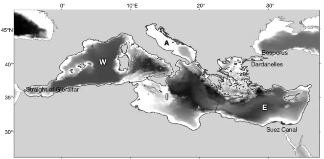
The Mediterranean Sea extends from 30° to 45° N and from 6° W to 36° E, and constitutes the world’s largest (2 522 000 km2_{) and deepest (average 1460 m,} maximum 5267 m) enclosed sea. It is connected to the Atlantic Ocean via the Strait of Gibraltar in the west, to the Black Sea via the Bosporus and the Dar-danelles in the north-east, and to the Red Sea via the Suez Canal in the south-east (Fig. 1). Overall, the basin is considered oligotrophic with some excep-tions along coastal areas due mainly to river dis-charges (Barale & Gade 2008) and frontal mesoscale activity (Siokou-Frangou et al. 2010). Phosphorus, rather than nitrogen, is the limiting nutrient, espe-cially towards the eastern basin (Krom et al. 1991). Biological productivity decreases from north to south and west to east, whereas an opposite trend is ob -served for temperature and salinity. In particular, the mean sea surface temperature varies between a min-imum of 14−16°C (west to east) in winter and a

max-imum of ca. 20−26°C (west to east) in the summer (with the exception of the shallow Adriatic Sea, where the range is between 8−10°C in winter and 26−28°C in summer) (Barale & Gade 2008). Evapora-tion greatly exceeds precipitaEvapora-tion, and river runoff de creases from west to east, causing sea surface height to decrease and salinity to increase eastward (Coll et al. 2010). The Mediterranean Sea has a topo-graphically diverse continental shelf that generally varies from south (mainly narrow and steep) to north (wider areas). In some instances, however, narrow shelves can also be found on some coasts of Turkey, in the Aegean, Ligurian and northern Alboran Seas, while extended shelves are also present on the Tunisian shelf and near the Nile Delta (Pinardi et al. 2006). Shelf waters represent 20% of the total Mediterranean surface, and the rest is open sea (Coll et al. 2010).

Mediterranean marine species richness is rela-tively high; to date, approximately 17 000 species have been recorded in the Mediterranean Sea, with a gradient of species richness that decreases from northwest to southeast (Bianchi & Morri 2000, Coll et al. 2010, 2012). Of these 17 000 species, at least 26% are prokaryotic (Bacteria and Archaea) and eukary-otic (protists) marine microbes. The phytoplankton community is composed predominantly of coccolitho-phores, dinoflagellates and Bacillariophyceae and includes more than 1500 species. Among microzoo-plankton, foraminiferans comprise the main group, with more than 600 species. However, the majority of species are described within the Animalia (~11 500

species), with the greatest contribution coming from the Crustacea (13.2%) and Mollusca (12.4%) (Coll et al. 2010). Among the vertebrates, 650 species of mar-ine fishes have been recorded, of which approxi-mately 80 are elasmobranchs and the rest are mainly actinopterygians (86%) (Coll et al. 2010). Nine spe-cies of marine mammals (5 Delphinidae, 1 Ziphiidae, 1 Physeteridae, 1 Balaenopteridae and 1 Phocidae) and 3 species of sea turtles (the green turtle Chelonia mydas, the loggerhead Caretta caretta and the leath-erback Dermochelys coriacea) are encountered regu-larly in the Mediterranean Sea. Among seabirds, 15 species frequently occur in the Mediterranean Sea, including 10 gulls and terns (Charadriiformes), 4 shearwaters and storm petrels (Procellariiformes) and 1 shag (Pelecaniformes) (Coll et al. 2010).

Ecosystem modelling approach

Two food web models of the entire Mediterranean Sea were constructed using the EwE software ver-sion 6 (Christensen et al. 2008) representing annual average biomasses and trophic flows for the 1950s and the 2000s. The analysis was restricted to Ecopath, the static component of the software that de -scribes the ecosystem and its resources at a precise period in time (Christensen & Walters 2004). In Eco-path, all principal autotroph and heterotroph species can be represented either individually or aggregated into functional groups considering their ecological roles.

Fig. 1. Mediterranean Sea, showing depth profile (darker shading indicates greater depth) and the 4 Marine Strategy Frame-work Directive (MSFD) areas: Western Mediterranean Sea (W); Adriatic Sea (A); Ionian and Central Mediterranean Sea (I);

The EwE model is based on 2 main equations. In the first one, the biological production of a functional group is equal to the sum of fishing mortality, preda-tion mortality, net migrapreda-tion, biomass accumulapreda-tion and other unexplained mortality as follows:

(1) where P/B is the production to biomass ratio for a cer-tain functional group i, Biis the biomass of a group i,

Yiis the total fishery catch rate of group i, (Q/B)jis the

consumption to biomass ratio for each predator j, DCji

is the proportion of group i in the diet of predator j, Ei

is the net migration rate (emigration − immigration), BAiis the biomass accumulation rate for the group i,

EEiis the ecotrophic efficiency, and (1 − EEi)

repre-sents mortality other than predation and fishing. In the second equation, the consumption (Q) of a functional group (i) is equal to the sum of production (P), respiration (R) and unassimilated food (GS × Q).

Qi= Pi + Ri+ GSi× Qi (2)

The implication of these 2 equations is that the model is mass balanced; under this assumption, Eco-path uses and solves a system of linear equations (1 for each functional group present in the system) esti-mating the missing parameters.

To ensure the mass balance, we applied a manual mass-balanced procedure following a top-down ap-proach, adjusting the input parameters of those groups ‘out of balance’ (EE > 1), occurring when total energy demand placed on those groups either by predation or fishing exceeds total production. In particular, we changed those parameters associated with higher un-certainty, i.e. diet matrix, P/B and, to a lesser extent, biomass (Christensen & Walters 2004). The ecological models were considered balanced when (1) estimated EE values were <1; (2) gross food conversion efficiency (P/Q) was < 0.5; and (3) respiration over assimilation (R/A) was <1 (Christensen & Walters 2004).

Parameterization and functional groups

Two food web models were constructed for the decades of 1950 and 2000, respectively. The reason for choosing these 2 time periods was related to best data collection in the case of the last decade and available catch time series (starting in the 1950s) and biogeochemical/stock assessment model outputs (e.g. biomasses for phytoplankton and fish stocks) for the first decade. To best represent the entire

Medi-terranean Sea ecosystem, while still considering sub-regional differences in environmental and bio-logical characteristics, both models were divided in 4 sub-models following the 4 sub-regional divisions defined by the Marine Strategy Framework Directive (MSFD; 2008/56/EC): (1) Western Mediterranean Sea (W); (2) Adriatic Sea (A); (3) Ionian and Central Mediterranean Sea (I); (4) Aegean and Levantine Sea (E) (Fig. 1). To separate each MSFD area within the full single Mediterranean model, we assigned a habi-tat area which corresponds to the fraction of the total area where the functional groups occur. In particular, if a functional group occurs throughout the total Mediterranean Sea, the biomass is scaled by a factor of 1; otherwise biomass is scaled by the fraction of the Mediterranean Sea area occupied (see Tables S1 & S2 in the Supplement at www. int-res. com/ articles/ suppl/ m533 p047_ supp. pdf).

To define functional groups, we used all available data to parameterize the model and ecological traits of species to establish the groups (see Tables S1−S4 in the Supplement).

We divided marine mammals into ‘piscivorous ceta ceans’ (mainly dolphins), ‘other cetaceans’ (mainly whales) and ‘pinnipeds’ (monk seal Mona chus monachus).

Fishes were divided into ‘sharks’, ‘rays and skates’, ‘deep-sea fishes’ (mainly mesopelagic, bathypelagic and bathydemersal), pelagic fishes and demersal fishes. Pelagic and demersal fishes were further divided in ‘small’ (common total length <30 cm), ‘me -dium’ (30− 89 cm) and ‘large’ (≥90 cm) following a similar approach used by Christensen et al. (2009), which simplified the definition of the fish groups (e.g. piscivores, benthivores and herbivores) in the model parameterization but still considered fish based on their asymptotic length, feeding habitats and vertical distribution characteristics. Invertebrate species were separated into ‘benthopelagic’ and ‘benthic cepha lo -pods’, ‘bivalves and gastro-pods’, ‘crusta ceans’, ‘jelly-fishes’, ‘benthos’ and ‘zooplankton’. Primary produc-ers were divided in ‘phytoplankton’ and ‘seagrass’. Each MSFD area had the same functional group cate-gories except for highly migratory species such as the ‘other cetaceans’ group, the ‘large pelagic fishes’ (e.g. tuna species and swordfish Xi phi as gladius) and the ‘sea turtles’ that were allowed to move and feed in all 4 areas. ‘European hake’ Merluccius merluccius, ‘Eu-ropean pilchard’ Sardina pilchardus and ‘Euro pean anchovy’ Engrau lis encrasicolus were considered in-dividually due to their importance as commercial spe-cies, and thus individual groups were created to rep-resent these species within the model. A total of 103

P B B Y B Q B DC E BA P B B EE i i i j j ji i i i i i j ( / ) ( / ) ( / ) (1 )

∑

× = + × × + + + × −

functional groups were described to represent the whole Mediterranean Sea model.

For each group, 5 input parameters were estimated: biomass (B), production rate per unit of biomass (P/B), consumption rate per unit of biomass (Q/B), diet composition (DC) and fisheries catch rate (Y). The bio -mass of each functional group, expressed as tonnes (t) of wet weight per km2_{, was obtained from field} sur-veys, estimated from empirical equations of popula-tion reconstrucpopula-tion or assessed by biogeochemical models. For the scope of this work, we searched mainly for data available at regional scales (either from survey campaigns or from other model outputs), and when this information was not available, local case studies were used instead (e.g. ‘seagrass’ bio-mass; see Tables S1 & S2 in the Supplement). For the 1950s model, which lacked surveyed data, the bio-masses of commercially important groups (functional groups 6 to 21 in Table 1) were estimated from stock as sessments (e.g. International Commission for the Conservation of Atlantic Tunas (ICCAT; https:// www. iccat.int/en/pubs_CVSP.htm for the large pelagic fishes) or by applying a logistic growth model (Schaefer 1954) as in previous studies (Walters et al. 2008, Piroddi et al. 2010). In particular, this last method, also called surplus production model, expressed as:

Nt +1= Nt+ rNt(1 − Nt/k)− Ct (3)

allows estimating the size of a given population/stock (N ) at certain time (t) knowing the historical catch time series (Ct), the intrinsic rate of population

growth (r; obtained from Fishbase, Froese & Pauly 2010) and the carrying capacity (k).

‘Phytoplankton’ biomass was taken from the out-puts of a biogeochemical model developed for the entire Mediterranean Sea (Macias et al. 2014), while ‘zooplankton’ was obtained from a global database available from the National Oceanic and Atmo -spheric Administration (www.st.nmfs.noaa.gov). For the other functional groups, information was avail-able either through the literature (e.g. ‘pinnipeds’ and ‘sea turtles’) or reconstructed from global databases (e.g. seabird biomass from the Sea Around Us Pro-ject; www.seaaroundus.org). The P/B and Q/B ratios were estimated using empirical equations (Chris-tensen et al. 2008) or taken from the literature and were expressed as annual rates (t km−2_yr−1_{) (Tables} S1 & S2 in the Supplement). A diet composition matrix was constructed using either field studies (e.g. stomach contents) or diet data obtained from the lit-erature for the same species in similar ecosystems (Table S3 in the Supplement). For highly migratory species (‘large pelagic fishes’, ‘other cetaceans’ and

‘sea turtles’) and ‘seabirds’ groups, we accounted for a percentage of the diet being outside the marine ecosystem, assuming that those species also move outside the studied system for feeding (Coll et al. 2006, 2007, Christensen et al. 2008, Piroddi et al. 2010). In some instances, we integrated parameters (B, DC, P/B and Q/B) from previously built EwE models for different areas of the Mediterranean Sea (Adriatic Sea: Coll et al. 2007, 2009c; Catalan Sea: Coll et al. 2006, 2008, Tecchio et al. 2013; Ionian Sea: Piroddi et al. 2010, 2011, Moutopoulos et al. 2013; Aegean Sea: Tsagarakis et al. 2010; Gulf of Lions: B˘anaru et al. 2013; Tunisia: Hattab et al. 2013). In particular, the output of these models was used as a starting point for the reconstruction of those parameters for which information was lacking. Detailed descriptions of the functional groups and data used to parameterize the model are given in Tables S1−S5 in the Supplement. No. Functional groups/fisheries Abbreviation 1 Piscivorous cetaceans PC 2 Other cetaceans OC 3 Pinnipeds PI 4 Seabirds SB 5 Sea turtles ST 6 Large pelagic fishes LP 7 Medium pelagic fishes MP 8 European pilchard EP 9 European anchovy EA 10 Other small pelagic fishes SP 11 Large demersal fishes LD 12 European hake HK 13 Medium demersal fishes MD 14 Small demersal fishes SD 15 Deep-sea fishes DF 16 Sharks SK 17 Rays and skates RS 18 Benthopelagic cephalopods BPC 19 Benthic cephalopods BC 20 Bivalves and gastropods BG 21 Crustaceans CR 22 Jellyfish JF 23 Benthos BE 24 Zooplankton ZO 25 Phytoplankton PH 26 Seagrass SE 27 Discards DS 28 Detritus DE 29 Trawlers TR 30 Dredges DR 31 Mid-water trawlers MT 32 Purse seiners PS 33 Long liners LL 34 Artisanal fisheries AR 35 Recreational fisheries RC Table 1. Functional groups and fisheries included in the

The official landing data by species and by country were taken from the United Nation’s Food and Agri-culture Organization (FAO) database (FishStat: http:// data.fao.org/database?entryId=babf3346-ff2d-4e6c-9a40-ef6a50fcd422) and available from 1950 to 2010. This time series was then complemented with data (available per country) from the Sea Around Us data-base (www.seaaroundus.org) to assign species to fishing fleet. We considered 6 commercial fisheries de -fined by gear types: bottom trawlers, bottom dredges, mid-water trawlers, purse seiners, long liners and the artisanal fisheries. Species were assigned to the fol-lowing gear types by assuming the same proportion per year as observed in the Sea Around Us database (data accessed in November 2013). In the case of Italy, which is surrounded by 3 of the 4 MSFD areas, we used a de tailed reconstruction of catches (Piroddi et al. 2014) available for sub- regional seas ([MFSD area 1] Ligurian; [2] Northern, Central and Southern Tyrrhen-ian; [3] IonTyrrhen-ian; [4] Northern, Central and Southern Adriatic Sea; [3] Sicilian; and [4] Sardinian waters), while for Greece, which has waters both in the Ionian and in the Eastern Mediterranean Sea, we used the same proportions as calculated by Tsikliras et al. (2007, 2013a). A recreational fishery was also included in the analysis using data coming from the Sea Around Us database (in the case of Italy and Spain) and from literature reviews (Anagno poulos et al. 1998, Gordoa et al. 2004, Pawson et al. 2007, Cis-neros-Montemayor & Sumaila 2010). We estimated the percentage of discards and the species discarded using reports and scientific papers available in the lit-erature (Megalofonou 2005, EC 2011, Vassilopoulou 2012, Tsagarakis et al. 2013) and data from previous EwE Mediterranean models available cited above. Fisheries landings and discards, expressed as annual rates (t km−2_yr−1_{), for both mo dels and for each} sub-region are shown in Tables S8− S11 in the Supplement. A list of functional groups and fisheries included in both models, to gether with their abbreviations, is given in Table 1 and in Table S5.

Pedigree index and model quality

The pedigree of the data refers to the uncertainty associated with the input values of the model. In gen-eral, higher pedigrees are associated with higher lev-els of data quality and with data coming from the study areas. Ecopath can take the pedigree values for all of the data entered in the model (e.g. biomass, P/B, Q/B, diets) into account and can calculate an overall pedigree index, ranging from 0 to 1. Lower

pedigree values imply a model constructed with low-precision data and with data coming from areas out-side the studied region, while higher values indicate a model constructed with locallyderived data (Moris -sette 2007, Christensen et al. 2008). Thus, to assess the quality of our input data, we calculated the over-all pedigree index for both models. In addition, the pedigree was also used to guide the balancing proce-dure of both models, such that the lower pedigree inputs were the first to be modified while balancing the models.

Model analysis and indices

Trophic flows in terms of total production, consump-tion, respiraconsump-tion, catches and flow to detritus were esti-mated to represent ecosystem structure and exploita-tion status (Odum 1969, Ulanowicz 1986, Christensen & Pauly 1993). In particular, the following indicators were evaluated: (1) Total system throughput (TST), calculated as the sum of all flows as an indication of the whole ecosystem size. (2) Total primary production/ total system respiration (TPP/ TR) and total primary production/total biomass (TPP/ TB), as a metric of sys-tem maturity. (3) Finn’s cycling index (FCI), as the per-centage of flows recycled in the food web (Finn 1976), and the predatory cycling index (PCI), as the percentage of production recycled after the removal of de -tritus (Christensen et al. 2008). (4) Ascendancy (A), as a measurement of system growth and development of network links (Monaco & Ulanowicz 1997). (5) Over-head (O), as the energy in reserve of an ecosystem that reflects the system’s strength when it experiences un-expected perturbations (Ulanowicz 1986). (6) System omnivory index (SOI), based on the average omnivory index (OI), which is calculated as the variance of the trophic levels (TLs) of a consumer’s prey groups indi-cating predatory specialization (Christensen & Pauly 1993). (7) Mean transfer efficiency (TE), as the effi-ciency in which energy is transferred between TLs. The mean TE is calculated as the geometric mean of TE for each of the integer TLs II to IV. (8) TL of each functional group expressed as:

(4) where j is the predator of prey i, DCjiis the fraction of

prey i in the diet of each predator j, and TLiis the TL

of prey i. By definition, TL I is attributed to primary producers and detritus, TL II to herbivores, TL III to first-order carnivores and TL IV to second-order car-nivores. (9) TL of the catches (TLC), as:

TLj DCji TL i n i 1 1

∑

= + ⋅ =

(5)

where Yirefers to the landings of species (group) i.

(10) Primary production required (PPR) to sustain the catch, to evaluate the sustainability of fisheries (Pauly & Christensen 1995).

To better represent trophic flows, TLs and bio-masses of the Mediterranean marine ecosystem, we used 2 different graphical representations: a flow diagram and a Lindeman spine (Lindeman 1942, Ula -no wicz 1995). In the Lindeman spine, primary pro-ducers and detritus (both with TL = 1) were separated to better represent the different flows going to the different compartments. To highlight differences in total biomass and mean TL of the community, we also plotted these 2 variables for each MSFD area for the 2 time periods.

Mixed trophic impact and keystone species analyses

The mixed trophic impact (MTI) analysis, ex -pressed as:

MTIij= DCij− FCji (6)

where DCijis the diet composition term expressing

how much j contributes to the diet of i, and FCjiis the

proportion of predation on j that is due to i as a pred-ator, allows the quantification of the impacts that a theoretical change of a unit in the biomass of a group (including fishing activities) would have on other groups in the ecosystem (Christensen et al. 2008). It can assess both direct and indirect trophic impacts in the food web, which are either positive or negative, indicating an increase or de crease in the quantity of the affected group. Here we looked at the MTI for each MSFD area and for the 2 different time periods. In addition, and building from the MTI analysis, the keystoneness index (KS) assesses the potential roles of each functional group as keystones in the system. Normally, keystone species are species with a rela-tive low biomass but whose biomass changes would have a disproportionately large effect on the ecosys-tem structure (Power et al. 1996). Here, for both time periods, we used the index proposed by Libralato et al. (2006):

KSi= log(εi× 1/pi) (7)

where εiis the overall effect expressed as the square

root of the sum of mijsquare (with mijbeing the

rela-tive impact of a slight increase in biomass of impact-ing group i on biomass of impacted group j), and piis

the contribution of the functional group to the total biomass of the food web.

Comparison with other European regional seas models

In an effort to support the MSFD, we compared a selection of ecological, fishing and network analysis indicators derived from the Mediterranean Sea model with those obtained from Ecopath models built for other European regional seas: the North Sea (Mackinson 2014), the Baltic Sea (Tomczak et al. 2012, 2013) and the Black Sea (Akoglu et al. 2014). This comparative analysis was done to obtain an overview, at the European scale, of similarities and differences between these exploited ecosys-tems. We are aware that a few limitations in con-fronting these models may occur due to differences in model criteria and construction (e.g. definition of certain groups, time periods), and for this reason we present model results with structural differences of the models for a better interpretation of the analysis. In addition, only those indicators more robust to model configurations (e.g. TST, mean TL of the catch, PPR to sustain fisheries, ascendancy and overhead; see Table 2 for the complete list of indicators), as previously assessed by Moloney et al. (2005) and Heymans et al. (2014), were used for the comparison.

RESULTS

Functional group input, data quality and mass balancing

Each MSFD area had 26 living groups (i.e. exclud-ing detritus and discards), if we also consider the 3 migratory groups as part of each area. Of those 26 groups, the main mass-balancing problems were en countered among ‘other small’ and ‘medium’ pe -lagic fishes, ‘small’ and ‘medium’ demersal fishes, ‘European pilchard’ and ‘an chovy’, ‘bentho pe la gic cephalopods’, ‘crustaceans’, ‘benthos’ and ‘zooplank-ton’, with EE values >1. To obtain mass balance for these groups, we primarily adjusted the diet matrix as the data source with higher uncertainty. For instance, the predation caused by ‘large pelagic fish’ on ‘European pilchard’ and ‘anchovy’, ‘medium’ and ‘other small’ pelagic fishes and ‘bentho pelagic

TL TL Y Y C i i i n i i i n 1 1

∑

∑

= ⋅ = =

cephalo pods’ was too high and was reduced. Similarly, the consumption of ‘other ceta ceans’, ‘bentho pelagic’ and ‘benthic ce pha lo pods’, ‘large’ and ‘me -dium demersal fishes’, ‘sharks’ and ‘rays and skates’ on the ‘crusta ceans’ group was overestimated and was reduced by redistributing the proportions in the predators’ diets. Biomasses of ‘crusta ceans’ and ‘bi -valves and gastropods’ were the only biomasses that were modified from the original input data. The bio-masses of these groups were indeed too low and had to be increased. This is a common problem in pre-balanced EwE models, where invertebrate biomass estimates are frequently too low to support predation mortality (Christensen et al. 2008).

Once balanced, EE values were high for the major-ity of the functional groups, indicating that total mor-tality in the system was mainly driven by predation and fishing. The gross food conversion efficiency (P/Q) and the respiration over assimilation (R/A) were within the expected ranges (Christensen et al. 2008). The resulting output parameters and the final diet matrix are shown for each model in Tables S1−S4 in the Supplement.

Pedigree indices were different for each time period and increased from the 1950s (0.391) to the 2000s (0.594). Individual results of the pedigree index can be found in Table S7 in the Supplement.

TLs and flows

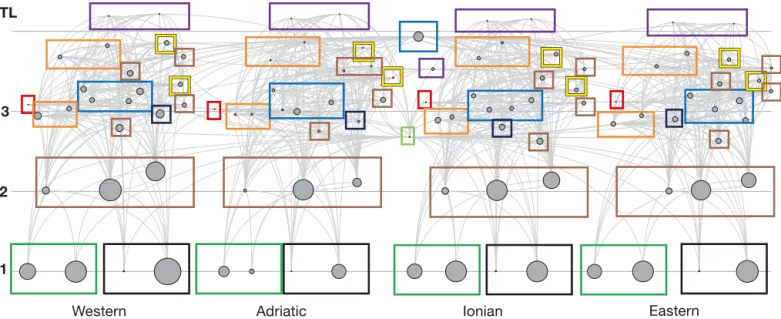
Trophic flows, TLs and relative biomasses of the Mediterranean Sea ecosystem for the 2000s model are represented in Fig. 2 andin Table S6 (flow

dia-grams) in the Supplement. In the latter, flow

dia-grams are separated for each MSFD area. Functional groups are illustrated by their TLs ranging from 1 (primary producers) to 4.22 (marine mammals); the highest TLs were found for ‘piscivorous cetaceans’ and ‘monk seals’ (TL ≥ 4). The other marine mammal group, ‘other cetaceans’, showed a TL of 3.53 (mainly because of the presence of ‘zooplankton’ and ‘ben-thopelagic cephalopods’ in their diet). ‘Seabirds’, despite being considered a top predator, showed a relatively low TL due to the presence of discards (mainly small pelagic fishes, Oro & Ruiz 1997, Boz-zano & Sardà 2002) in their diet. Similarly, ‘sea tur-tles’ might have a higher TL than estimated by the model, but their diet also includes discards (Tomas et al. 2001, Gómez de Segura et al. 2003, Casale et al. 2008), and thus, they presented a fairly low TL (2.68) in the model. This is an artifact of EwE that considers discards as a detritus group with TL = 1 and thus tends to lower the TL of those groups that feed con-siderably on discards (Christensen et al. 2008), as previously seen in other food web models of

Mediter-TL

3

2

1

Western Adriatic Ionian Eastern

Fig. 2. Flow diagram of the Mediterranean Sea ecosystem (in the 2000s) with the Western part being at the far left followed by the Adriatic, the Ionian and the Eastern (see Fig. 1). Each functional group is shown as a circle whose size is approximately pro-portional to the log of its biomass. All functional groups are represented by their trophic levels (TL; y-axis) and linked to each other by predator−prey relationships expressed as light grey lines. Coloured boxes define the main functional groups: marine mammals (purple); pelagic fishes (blue); demersal fishes (orange); sharks/rays and skates (yellow); deep-sea fishes (dark blue); seabirds (red); invertebrates (brown); sea turtles (light green); primary producers (dark green); detritus groups (black). Individ-ual flow diagrams of the 4 Marine Strategy Framework Directive (MSFD) areas are presented in Table S6 in the Supplement at

ranean areas (Coll et al. 2006, 2007, Piroddi et al. 2010). For the fish groups, ‘large pelagic fishes’ showed a relatively high TL (3.94), followed by ‘European hake’ (between 3.86 and 3.73), ‘large demersal fishes’ (between 3.68 and 3.56), ‘sharks’ (be tween 3.85 and 3.64) and ‘rays and skates’ (between 3.41 and 3.27). ‘Medium’ and ‘other small’ pelagic fishes were given a TL between 3.28 and 3.19 and be tween 3.14 and 2.89, respectively. ‘European pil chard’ and ‘European ancho vy’ had TL values ranging between 3.25 and 3, while the lowest TLs were observed for ‘medium’ and ‘small’ demersal fishes and ‘deep-sea fishes’ (be tween 3.04 and 2.80). Of the remaining functional groups, ‘benthopelagic’ and ‘benthic cephalopods’ and ‘jellyfish’ reached TL >3, ‘crustaceans’ showed values between 2.79 and 2.63, and ‘zooplankton’, ‘bivalves and gastropods’ and ‘benthos’ had TL values close to 2.

Looking at the 4 MSFD areas, comparing total bio-mass and mean TL of the community, the Adriatic and the Western Mediterranean Sea were the areas with the highest total biomass, followed by the Ionian and Eastern Seas (Fig. 3). During the 2000s, the mean TL of the community (TLco) differed considerably whether calculated using TLco ≥ 1 or TLco > 1 (i.e. excluding detritus and primary producers). For TLco ≥ 1, the Adriatic was the area with highest mean TLco (1.86) followed by the Ionian (1.56), Eastern (1.5) and Western Mediterranean (1.49). For TLco > 1, the Western had the highest TLco (2.36), followed by the Eastern (2.34), Ionian (2.28) and Adriatic Seas

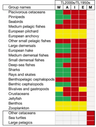
(2.18) (Fig. 3). Several differences in TLs were also found between the 2 modelled time periods, with declines observed particularly in the Ionian and East-ern Mediterranean Sea in the 2000s compared to the 1950s (Fig. 4). However, to be able to assess changes in TL of the community in the Mediterranean Sea, a more accurate analysis is needed (such as fitting the model to time series data that will reduce the noise around the parameters; Christensen & Walters 2004). In the Lindeman spine analysis (Fig. 5), similar pat-terns were observed for both time periods. Most trophic flows fell within TL I, II and III, and TL I was the pool that generated the majority of the total sys-tem throughput (1950s: 78.4% and 2000s: 79.3%) fol-lowed by TL II, with 20.2% for the 1950s and 19.6% for the 2000s. In both time periods, primary produc-ers and TL II organisms had the highest biomasses, and comparing the 2 decades, a decline in biomasses was observed in the 2000s versus the 1950s particu-larly for those groups having TLs higher than III. In both systems, exports as catches were mainly con-centrated within TL III.

Fig. 3. Total biomass and mean trophic level of the commu-nity (TLco) with and without detritus and primary producers (TLco > 1) for each MSFD area (see Fig. 1) for the 2000s. Total biomass is shown as a circle whose size is proportional

to the area of the MSFD

Fig. 4. Changes in trophic levels (TLs) between the 1950s and the 2000s for each functional group for each Marine Strategy Framework Directive (MSFD) area (W: Western; A: Adriatic; I: Ionian/Central; E: Aegean/Levantine) and the whole Mediterranean Sea (M: Mediterranean). Green cells represent increased TLs (> 0), yellow cells indicate stable TLs (=0), and red cells show decreased TLs (< 0).

Trophic impact and keystone species

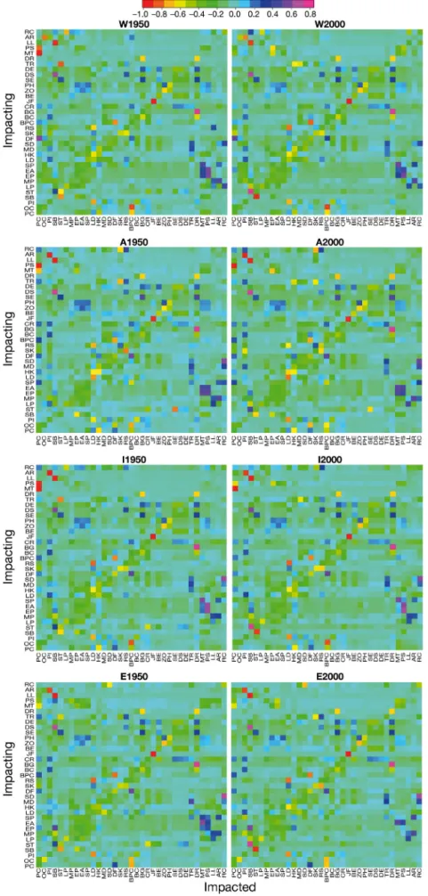
For a better interpretation of the MTI analysis, re-sults are presented separating each MSFD area (Fig. 6). Several general patterns can be observed in all 4 areas. Among all MSFD areas, most predators had a direct negative impact on their prey through their diet preferences; functional groups negatively impacted themselves due to cannibalism/ within-group competition; demersal functional within-groups had a greater impact (either negatively or positively) on the majority of the other groups than pelagic functional groups, and ‘zooplankton’ and ‘phyto plankton’ groups most positively affec ted all other groups in the system (e.g. through a bottom-up effect).

MTI analysis in both time periods re vealed changes in the role of ‘pinni peds’ in the West, Adri-atic and Ionian Seas, with a higher impact in the food web during the 1950s and almost no impact in the 2000s. In the Eastern Mediterranean, where the spe-cies still oc cur red in greater numbers, the im pact on the food web was greater in 2000s than in the other 3 MSFD areas but still reduced compared to the 1950s. Similar trends were observed for ‘piscivorous ceta -ceans’ in all MSFD areas, where the group had a large effect in the 1950s but because of their reduced biomass, only had a limited effect in the 2000s. For fishes, ‘European anchovy’ and ‘European pilchard’

similarly affected the Mediterran-ean food web with greater positive impact on top predators, pelagic fishes and fisheries (particularly mid-water trawlers and purse sein-ers). Interestingly, ‘sharks’ were negatively impacting marine mam-mals either through direct competi-tion for the same resources or niche overlap. Overall, lower TL organisms, namely ‘benthos’, ‘crusta -ceans’ and particularly ‘seagrass’, positively affected the rest of the food web.

Results also revealed that the role of fisheries in the different MSFD areas has changed with time, grow-ing in impact from 1950s to 2000s, and affecting several groups in the different food webs. In general, if only the commercially exploited functional groups were considered, results showed a greater impact of bottom trawlers, mid-water trawlers and purse seiners (Fig. 7b). More specifically, bottom trawlers and dredges had large negative impacts on targeted demersal species (mainly demersal fishes and ‘molluscs’) and on ‘sea turtles’ (incidental catches), while longline fisheries had large negative impacts on ‘large pelagic fishes’ (target species) and, through incidental catches, on ‘sea turtles’, dolphins and ‘seabirds’. Mid-water trawlers and purse seiners showed negative impacts on targeted small pelagic fishes and, through direct competition for the same resources, on marine mam-mals and ‘seabirds’. When all functional groups in the ecosystem were included in the analysis, arti-sanal fisheries seemed to be the fleets with greater negative impact, particularly in the Western, Ionian and Eastern Mediterranean Seas (Fig. 7a). Recre-ational fisheries had a negative impact on ‘large pelagic fishes’ and ‘sharks’ in the Western, Adriatic and Ionian Seas and on ‘medium’ and ‘small’ demer-sal and ‘medium‘ and small pelagic fishes in the Eastern Mediterranean.

The results obtained from the keystoneness analysis (Fig. 8 and Table S6 in the Supplement) revealed that in the 1950s ecosystem, ‘large pelagic fishes’ had the highest overall keystoneness role followed by ‘sharks’ and ‘medium pelagic fishes’ groups, whereas in the 2000s ecosystem, ‘medium pelagic fishes’ were re-placed by ‘benthic’ and ‘bentho pelagic cephalopods’. Interestingly lower TL groups (e.g. ‘zooplankton’,

P

40.78 18.43 519.0

II

20.16 22.29 0.0371 267.7 44.41 0.0628

III

1.268 5.200 0.187 28.25 4.617 0.108

IV

0.135 1.037 0.0230 3.004

D

37.64 20.76 913.2 396.0 11.47 1.195 1322 189.1

P

41.47 16.03 613.7

II

19.60 21.23 0.0920 263.2 39.91 0.0526

III

1.031 4.446 0.511 24.13 4.033 0.114

IV

0.108 0.905 0.0526 2.532

D

37.78 20.18 996.6 457.9 11.36 1.125 1467 147.4

TL

TST(%) Biomass

Exports and catches

Respiration Consumption Predation TE Flow to detritus Flow to detritus

a

b

Fig. 5. Lindeman spine representation of trophic flows (t km−2 _yr−1_{) and biomasses (t}

km−2_{) for the entire Mediterranean Sea}

ecosys-tem for (a) the 1950s and (b) the 2000s. P: pri-mary producers; D: detritus (both TLI). TST%: total system throughput; TE: transfer efficiency

‘phytoplankton’ and ‘benthos’) were also identified in both time periods as keystone groups, probably caused by their overall low biomass and high P/B (characteristic of oligotrophic systems) and important role in the ecosystem. In both time periods, marine mam-mals, in particular ‘pinnipeds’ and ‘pisci vorous cetaceans’, appeared within the least important keystone groups.

Comparison among European regional seas

The statistics and main indicators calculated from the whole Mediter-ranean Sea ecosystem model repre-senting the 2000s were compared with other modelled European re -gional seas for the same or similar period (Table 2). The TST revealed that the main flows driving the Medi-terranean Sea were flow to detritus (42%) and exports (39%) followed by consumption (15%) and respiration (5%). In the Baltic, North and Black Seas, on the other hand, consumption seemed to be the flow with the high-est importance (around 43−48%) fol-lowed by flow to detritus (22−30%), respiration (20−23%; in the Black Sea, this flow constituted the second most important flow, with 29%) and exports (1−6%).

Looking at ecological indicators ad-dressing community energetics and cycling of nutrients, under Odum’s theory (Odum 1969), our results

sug-Fig. 6. Mixed trophic impact relationships between functional groups and fisheries in the 4 different Marine Strategy Frame-work Directive (MSFD) areas (W: Western; A: Adriatic; I: Ionian/Central; E: Aegean/ Levantine). Positive values (from light blue to purple) indicate positive impacts; nega-tive values (from light green to red) indi-cate negative impacts. The colors should not be interpreted in an absolute sense: the impacts are relative, but comparable be-tween groups. For group abbreviations,

gest that the Mediterranean Sea eco-system is at an early developmental stage. This was visible, for example, in the ratio between total primary

pro-duction (PP) and total respiration (R)

(Odum 1969, Christensen 1995) or in the primary production/biomass ratio (PP/B). On the other hand, the indica-tors from the other European Seas suggested that systems fell within an intermediatelow level developmen -tal stage. For the SOI, despite the low general values, the Mediterranean Sea showed the highest value, while in relation to the 2 cycling indices, the Mediterranean basin had the highest values in PCI and the lowest in FCI. For each European regional sea, as-cendancy was relatively low, whereas –0.75 –1.75 –1.55 –1.35 –1.15 –0.95 –0.75 –0.55 –0.35 –0.15 0.05 –0.65 –0.55 –0.45 –0.35 –0.25 –0.15 –0.05 0.05 Trawlers W Dredges W Mid-water trawlers W Purse seiners W Long liners W Artisanal W Recreational W Trawlers A Dredges A Mid-water trawlers A Purse seiners A Long liners A Artisanal A Recreational A Trawlers I Dredges I Mid-water trawlers I Purse seiners I Long liners I Artisanal I Recreational I Trawlers E Dredges E Mid-water trawlers E Purse seiners E Long liners E Artisanal E Recreational E Impact 1950 Impact 2000

b

a

Fig. 7. Cumulative impact (either direct or through a cascade effect) of each fishing gear on (a) all functional groups of the eco-system and (b) all commercially important species/groups of the ecoeco-system (see Table 1, numbers 6 to 14 and 16 to 21), in the different Marine Strategy Framework Directive (MSFD) areas (see Fig. 1) and for each studied period. The cumulative impacts were calculated from the mixed trophic impact calculations. Negative values on the x-axis represent negative impact to a

positive change in fishery harvest

Fig. 8. Relative total impact (εi) versus

key-stoneness (KSi) showing the role of

spe-cies/groups in the ecosystem for both time periods (1950s and 2000s). The size of the circles is proportional to the species/group biomass. Functional groups that showed a decline in their keystone role in com -parison to the 1950s are shown in red. For

overhead was high. The mean TE observed in the Mediterranean Sea was similar to the Baltic Sea but was lower in comparison to values calculated for the Black and North Seas. As for fishing indicators, the PPR% of the Mediterranean was 0.81%, the lowest among the other seas, while TLcwas 3.04 in the

Medi-terranean Sea, similar to the Black Sea and lower in comparison to the other European Seas with higher TL values (between 3.3 and 3.7).

DISCUSSION

This study constitutes the first attempt to build an historical and current food web model for the whole Mediterranean Sea with the challenging effort to integrate available spatial and temporal (in terms of comparing the 1950s and 2000s) biological data and modelling outputs in a coherent manner. We acknowl edge that data gaps still exist, for example on temporal changes in diet composition, temporal estimates of discards and biomasses of non-commer-cially important species and deep-sea organisms. Thus, further efforts should be made to reduce this uncertainty and increase the quality of these models.

Quality of the models

As expected, the 1950s model showed a lower pedigree index, scoring in the lower range (0.164− 0.676) when compared to the 150 balanced EwE models previously assessed globally by Morissette (2007). This is because the 1950s model was con-structed using mainly data obtained from other mod-elling approaches (e.g. biogeochemical models to estimate phytoplankton biomasses and stock recruit-ment models to estimate biomass of fish stocks; refer to Table S5 in the Supplement for details of each functional group). Models that have tried to repre-sent the past have always been associated with higher uncertainty, as was observed in other studies (Coll et al. 2008, 2009c, Piroddi et al. 2010, Chris-tensen et al. 2014, Macias et al. 2014), and their out-puts should be always taken with caution. To limit this uncertainty, we tried to use models for which outputs have been tested and when possible vali-dated (Macias et al. 2014), or that have been widely utilized to assess temporal biomasses as done for fish stocks (e.g. surplus production models; Walters et al. 2008, Piroddi et al. 2011). In contrast, the 2000s model, due to its higher data quality, showed a rela-Indicators Mediterranean North Sea Baltic Sea Black Sea Units Sea (Mackinson (Tomczak (Akoglu

(this study) et al. 2014) et al. 2012) et al. 2014)

Main ecosystem features

Area 2512000 570000 240000 150000 km2

Studied period 2000s 1991 2000s 1995−2000 Year Functional groups 103 68 21 10 No. Main indicators

Sum of all consumption 923 6157 3435 4500 t km−2 _yr−1

Sum of all exports 1320 105 476 490 t km−2_yr−1

Sum of all respiratory flows 290 2658 1851 2990 t km−2_yr−1

Sum of all flows into detritus 1467 3867 2246 2230 t km−2_yr−1

Total system throughput 4000 12786 8007 10210 t km−2_yr−1

Mean trophic level of the catch 3.08 3.7 3.30 3 Gross efficiency (catch/net primary production) 0.00026 0.00226 0.0016 0.001 Total primary production 1610 2609 2434 3483 t km−2_yr−1

Total primary production/total respiration 5.55 0.98 1.26 1.16 Primary production required to sustain fisheries 1.46 5.88 52.57 28.93 %

(PPR, considering primary production)

Total primary production/total biomass 37.67 4.71 22.54 90 Total biomass (excluding detritus) 42.74 554 108 38.7 t km−2

Connectance index 0.10 0.22 0.22 2.5 System omnivory index 0.27 0.23 0.15 0.116 Predatory cycling index 10.96 – 0.41 – % Finn’s cycling index 4.98 20.24 6.98 15.01 % Mean transfer efficiency 9.2 30.2 12 7.4 % Ascendancy 42.9 20.6 30.82 31.7 % Overhead 57.1 79.4 69.18 68.3 % Table 2. Summary statistics for the Mediterranean Sea food web model in comparison with the North Sea, Baltic Sea and

tively higher pedigree. This was due to the availabil-ity, in more recent years, of survey data (e.g. trawl surveys such as the MEDITS campaign) and the increase in biodiversity assessments (e.g. Coll et al. 2010) that have improved the level of knowledge in the basin. Nevertheless, data deficiencies exist, particularly in African and Arabic countries, where survey data remain either inaccessible or absent. Despite these limitations, the models developed in this study represent an important step towards an integrated understanding of the Mediterranean Sea marine ecosystem structure and function.

Biomasses, trophic flows and TLs

Results presented here show how the Mediterran-ean Sea is mainly dominated, in terms of biomass, by lower TL organisms, particularly ‘benthos’, ‘zoo-plankton’ and ‘phyto‘zoo-plankton’. These groups domi-nate most of the system flows and, as ob served at smaller scales in other Mediterranean food web models (Coll et al. 2006, 2007, Tsagarakis et al. 2010, Moutopoulos et al. 2013, Torres et al. 2013), con-stantly appear as important key species. This is prob-ably because of the relatively low biomass at higher TLs and a relatively high mean TE overall in the food web, in line with previous studies (Pauly & Christensen 1995, Coll & Libralato 2012). This pheno -menon is called the ‘Mediterranean paradox’ for the fact that despite the oligotrophic condition of the basin that constrains the reproduction and feeding of zooplankton, the ecosystem is capable of producing a relatively high fish abundance (Sournia 1973, Macias et al. 2014). In addition, the high TEs have been sug-gested as a sign of overexploitation of the Mediter-ranean Sea due to high production exports (Coll et al. 2009b).

Marine mammals and large pelagic fishes, on the other hand, are the top predators of the ean marine ecosystem. In particular, the Mediterran-ean monk seal Monachus monachus is the species with the highest TL followed by ‘piscivorous ceta -ceans’ and ‘large pelagic fishes’. These outcomes are very interesting since the Mediterranean monk seal and several dolphin populations (e.g. the short-beaked common dolphin Delphinus delphis) have dramatically declined over the centuries because of a variety of anthropogenic pressures (e.g. fisheries interactions, habitat loss and pollution) and are now classified either as Critically Endangered (the Medi-terranean monk seal is almost extinct), Endangered, or Vulnerable by the International Union for

Conser-vation of Nature (IUCN) Red List of Threatened Ani-mals (UNEP/MAP 1994, Johnson & Lavigne 1998, Reeves & Notarbartolo di Sciara 2006, Bearzi et al. 2008, Piroddi et al. 2011).

Large pelagic fishes (mainly tuna species and swordfish), the main keystone group in our model-ling ap proach, have consistently been exploited for thousands of years in the Mediterranean Sea, and these species are also at low levels of abundance (Abdul Malak et al. 2011). This severe decline in bio-diversity at the top of the food web particularly in recent decades (Briand 2000, Bearzi et al. 2008, Coll et al. 2008, 2009c, Piroddi et al. 2010, 2011, Lotze et al. 2011), as also shown in our study by their reduced biomass levels, could have induced a cascade effect throughout the food web, with effects on the com-plexity, connectivity and robustness of the system against further species loss (Briand 2000, Heithaus et al. 2008, Lotze et al. 2011, Piroddi et al. 2011). De -fined as umbrella, sentinel, keystone or flagship spe-cies, they reflect ecosystem changes and degradation over time, as is also clear from our keystone and MTI analysis, and ensuring their survival would lead to ways of enhancing marine ecosystems and ensure sustainable human activities (Bossart 2006, Boyd et al. 2006, Trites et al. 2006, Sergio et al. 2008).

Ecological role of species and changes with time

The results of our keystone analysis for both time periods also revealed changes over time in other important keystone species. After ‘large pelagic fishes’, ‘sharks’ and ‘medium pelagic fishes’ have played a key role in the past ecosystem, replaced in more recent years by ‘benthopelagic cephalopods’. This is not the first time that cephalopods have been identified as a keystone group in Mediterranean food webs (Coll et al. 2006, Tsagarakis et al. 2010, B˘anaru et al. 2013, Hattab et al. 2013, Torres et al. 2013). This functional group, the role of which in the overall structure and functioning of marine ecosystems remains poorly understood, has an important trophic position (being both predator and prey), and because it can proliferate in highly exploited ecosystems, it constitutes a key element of present marine food webs (Pierce et al. 2008, Coll et al. 2013). As for ‘sharks’, particularly large predatory sharks, several studies have pointed at strong declines in species over the last centuries mainly due to intensive over-exploitation (both for consumption and as discarded species; Megalofonou 2005, Ferretti et al. 2008, May-nou et al. 2011, Coll et al. 2014a). The present study

suggests that these species were important in the past Mediterranean ecosystem and confirms a dimin-ishing role within the current food web as a conse-quence of a reduction in their abundance.

Small and ‘medium’ pelagic fishes, both with high biomasses and high proportions in catches, show an important role in the Mediterranean ecosystem as structuring species of the food web (Coll et al. 2006, 2007, Piroddi et al. 2010, Tsagarakis et al. 2010). Yet, our results highlight how these organisms, despite being essential for transferring energy from lower to higher TL organisms (Cury et al. 2000, Pikitch et al. 2014), have diminished considerably be tween the 2 time periods and between sub-regions, causing a reduction in their ecological role.

Fishing impact and the quality of data

From the MTI analysis, bottom trawling and dredges were the fisheries with the widest impact on the food web, particularly on the demersal commu-nity. This has been observed in sub-areas of the Mediterranean Sea representing continental shelf and upper slopes (Coll et al. 2006, 2007, B˘anaru et al. 2013, Hattab et al. 2013). Therefore, our results high-light the effect of bottom trawlers and dredges on marine resources and ecosystems of the Mediterranean Sea as an important issue that should be ad -dressed if sustainable management of fisheries is to be achieved within the region (Puig et al. 2012). The impacts of artisanal fisheries on the ecosystem have also increased over time, particularly in the Ionian and Eastern Mediterranean Seas, and are probably caused by increased fishing effort in the EU, north-ern Afri can and Arabic countries (Anticamara et al. 2011). This also has clear implications for the man-agement of marine resources in the Mediterranean Sea be cause the artisanal fleet dominates the fishing activity in many Mediterranean countries but is poorly monitored.

Overall, our results show that over time, fisheries have exerted a negative pressure on the food web as a consequence of increased and intensive over-exploitation. Yet, several interpretations of these results could be drawn: first, fisheries might not display a greater negative impact (than the one presented here) on commercially important species be cause of the inclusion in the analysis of develop-ing countries (e.g. North African and Arabic coun-tries) and developed countries together. Completely different spatiotemporal patterns/trends character-ize these 2 sides of the Mediterranean Sea that

might lead to a masking effect scenario. A reflection of this is visible in the increased impact of artisanal fisheries in the Ionian and Eastern Mediter ranean Seas, possibly as a consequence of increased fishing effort in southern Mediterranean countries. This distortion might also be caused by discards, which we kept constant in time due to lack of information, and by Illegal, Unregulated, and Unreported IUU) activities that, despite being a serious issue in the Mediterranean Sea (Ulman et al. 2013, Coll et al. 2014b), were not included in this study due to the lack of a global estimate for the Mediterranean Sea. Also, recreational catches are not included in national fishery statistics, and only re cently a Euro-pean Union legislation (Council Regulation [EC] No. 1224/2009) has required the survey of recre-ational fishing activities. Since only few sources of information exist, which have been incorporated into the model, catches may well have been under-estimated. Using fisheries statistics supplied to the FAO by individual countries could be another limit-ing factor. Several studies have indeed confirmed that most of these statistics largely underestimate their likely true catch by a factor of 2 or more (Zeller & Pauly 2007, Pauly et al. 2014). This could be particularly true for the Southern Mediterran-ean, where mechanisms to collect fisheries data are less available (FAO 2010) and for some Mediter -ranean countries where this factor is even higher (Pauly et al. 2014). An unrealistic scenario is also observed regarding mid-water trawling in the East-ern Mediterranean Sea, where this gear shows an impact on marine resources, despite the fact that it does not operate in most of the Eastern Mediter -ranean countries (Sacchi 2011). Obviously this is an error in the Sea Around Us project database, which at the time it was accessed was still under development.

These caveats represent the major weaknesses of the Mediterranean fisheries data, and some caution should be taken when interpreting the data. Cur-rently, a database on global fisheries reconstruction from 1950 to 2010, which aims at looking at all types of fisheries removals (from reported and unreported landings to recreational landings and discards) is being constructed, including Mediterranean coun-tries (Le Manach et al. 2011, Ulman et al. 2013, Coll et al. 2014b, Pauly et al. 2014). In the near future, this information on catch reconstructions could be inte-grated in modelling efforts to reduce the limitations explained above, and to capture better the fishing pressure on current and past Mediterranean marine ecosystems.

Similarities and differences among European regional seas

The relative total biomass per km2_{and per each} in-dividual sea reveals that the Adriatic and Western Mediterranean are the areas with the highest biomass followed by the Ionian and Eastern Mediterranean. This confirms a decrease gradient of richness from west to east, as observed in other studies (Bosc et al. 2004), influenced by changes in environmental pa-rameters (e.g. productivity, temperature and salinity) that define and characterize the Mediterranean Sea. Comparing our results to other European seas illus-trates that European regional seas are quite diverse. In particular, the Mediterranean Sea stands alone in relation to the type of flows that drive the system and the cycling indices that suggest higher levels of com-munity stress induced by intensive fishing activities, as previously illustrated (Costello et al. 2010).

In regards to ecosystems development, the Medi-terranean Sea appears to be in an early development stage, different from the other systems, probably because the ecosystem has been perturbed continu-ously over a long period of time. Indeed, when eco-systems develop, biomasses and complexity tend to increase and mature, whereas when they are dis-turbed, e.g. by fishing, they show the opposite trend and stay ‘young’ (Odum 1969).

One similarity with the other EU ecosystems is given by the TLs of the catches, which are low in the Mediterranean Sea, in the Black Sea and recently in the Baltic Sea (e.g. herrings and sprats have replaced the collapsed Eastern Baltic cod Gadus morhua in the landings; Tomczak et al. 2012), highlighting the im -portance of small pelagics in the fisheries activities of these areas. Although differences may have oc cur red in the way models were constructed (such as the number of functional groups and links), these out-comes are in line with other studies that pointed at differences in physical and biological features (from highly eutrophic with frequent hypoxia events to moderately eutrophic and productive or relatively oligotrophic regions; Coll et al. 2010, Tomczak et al. 2012, Mackinson 2014) as the reasons for these dif-ferences in diversity among European regional seas (Barale & Gade 2008, Narayanaswamy et al. 2013).

Concluding remarks

Overall, our study is the first to provide a basis for understanding and quantifying the structure and functioning of the whole Mediterranean Sea

ecosys-tem, including main marine organisms, from low to high TLs, and considering fishing activity. This is also the first Ecopath model that tries to integrate sub-regions within a unified model to take into consider-ation differences in biological and environmental characteristics. The construction of 2 food web mod-els (for the past and for current years) enabled us to assess changes in the food web and impacts (in this case fishing) affecting the system. However, further developments of spatial and temporal hind- and forecast analysis are necessary to further model the dynamics of the ecosystem (such as movements of species within and between areas and large migra-tions) and evaluate the exploitation status of the Mediterranean Sea and explore different manage-ment policies and future scenarios. Temporal simula-tions to hindcast food web dynamics have been developed in regional areas of the Mediterranean Sea such as the Catalan Sea (Coll et al. 2008), the Adriatic Sea (Coll et al. 2009c) and the Ionian Sea (Piroddi et al. 2010). Quantifying the impact of im -portant threats (e.g. climate change and fishing pres-sure) on a system that is considered ‘under siege’ (Coll et al. 2012) becomes critically important for ensuring the sustainability of marine resources and the services they provide to humans, and the conser-vation of this vulnerable ecosystem. This is a step further for the regional assessment of the Mediter-ranean Sea ecosystem.

Acknowledgements. M.C. was partially supported by a Marie Curie CIG grant — PCIG10-GA-2011-303534 — to the BIOWEB project and the Spanish Research Program Ramon y Cajal. V.C. acknowledges support from NSERC. We thank the 3 anonymous reviewers for their valuable comments and suggestions on the manuscript. We acknowledge all those colleagues from the Joint Research Centre (JRC) who pro-vided essential technical advice to the development of this work. Special thanks go to F. Somma, C. Liquete and L. Gur-ney for constructive comments on model construction and the draft manuscript; to S. Libralato and S. Heymans, who kindly advised on model development; to G. Notarbartolo di Sciara, A. Canadas, M. Rosso who provided data and/or important insights on marine mammals functional groups; and to M. Tomczak, E. Akoglu and C. Lynam, who provided European regional seas model-derived indicators.

LITERATURE CITED

Abdul Malak D, Livingstone SR, Pollard D, Polidoro BA and others (comps) (2011) Overview of the conservation sta-tus of the marine fishes of the Mediterranean Sea. IUCN, Gland

Akoglu E, Salihoglu B, Libralato S, Oguz T, Solidoro C (2014) An indicator-based evaluation of Black Sea food web dynamics during 1960−2000. J Mar Syst 134: 113−125

➤ ➤