by Yuan Cheng
M.S., Mechanical Engineering (1998) Massachusetts Institute of Technology
Submitted to the Department of Mechanical Engineering in Partial Fulfillment of the Requirements for the Degree of
Doctor of Philosophy in Mechanical Engineering at the
Massachusetts Institute of Technology December, 2000
Ci
00
@2000 Massachusetts Institute of Technology All rights reserved
Signature of Author
Certified by
Accepted by
I~
I
Department of Mechanical Engineering /December, 2000
C.Forbes Dewey, Jr. Professor of echanical Engineering Thesis Supervisor Ain A. Sonin OFTECHNOLOGY JUL 1 6 ?001
LIBRARIES
BARKER
by Yuan Cheng
Submitted to the Department of Mechanical Engineering on December 3 1st, 2000, in Partial Fulfillment of the
Requirements for the Degree of
Doctor of Philosophy in Mechanical Engineering
Abstract
Approaches to achieve three dimensional (3D) reconstruction from 2D images can be grouped into two categories: computer-vision-based reconstruction and tomographic reconstruction. By exploring both the differences and connections between these two types of reconstruction, the thesis attempts to develop a new technique that can be applied to 3D reconstruction of biological structures. Specific attention is given to the reconstruction of the cell cytoskeleton from electron microscope images.
The thesis is composed of two parts. The first part studies computer-vision-based reconstruction methods that extract 3D information from geometric relationship among images. First, a multiple-feature-based stereo reconstruction algorithm that recovers the 3D structure of an object from two images is presented. A volumetric reconstruction method is then developed by extending the algorithm to multiple images. The method integrates a sequence of 3D reconstruction from different stereo pairs. It achieves a globally optimized reconstruction by evaluating certainty values of each stereo reconstruction. This method is tuned and applied to 3D reconstruction of the cell cytoskeleton. Feasibility, reliability and flexibility of the method are explored.
The second part of the thesis focuses on a special tomographic reconstruction, discrete tomography, where the object to be reconstructed is composed of a discrete set of materials each with uniform values. A Bayesian labeling process is proposed as a framework for discrete tomography. The process uses an expectation-maximization (EM) algorithm with which the reconstruction is obtained efficiently. Results demonstrate that the proposed algorithm achieves high reconstruction quality even with a small number of projections. An interesting relationship between discrete tomography and conventional tomography is also derived, showing that discrete tomography is a more generalized form of tomography and conventional tomography is only a special case of such generalization.
Thesis Committee:
C. Forbes Dewey, Jr., Professor of Mechanical Engineering and Bioengineering Eric Grimson, Professor of Computer Science and Engineering
David Gossard, Professor of Mechanical Engineering
I am very proud of having the most important part of my life associated with the world's most prestigious engineering school, MIT. I am more grateful for the helps and supports that I received during this period of time from so many wonderful people around me.
First and foremost, I would like to thank my advisor, Professor C. Forbes Dewey for bringing me into his group and showing confidence in me and my work. His continuous encouragement, patience and guidance have shaped my research and helped me to overcome hurdles one after the other. I also thank him for a number of inspiring and productive discussions on the way to and back from Royal East.
I am thankful to my thesis committee members: Professor Eric Grimson, Professor David Gossard and Professor John Hartwig. It has been my special honor to have these world-known scientists in my thesis committee. I thank them for their presence, their support and numerous suggestions that they made towards my work. Special thanks to Professor Hartwig for tolerating my near ignorance of cell biology and helping me in preparing the
specimen.
I am also grateful to my present and past lab-mates for their helps. My improvement in English, if any, largely attributes to them. I would also like to thank Ms. Donna Wilker for her helps in past years and for her successful attempts to balance my research life by lending me her movie collections.
Finally, I dedicate this thesis to my parents who supports me unconditionally with their hearts and also to my loving wife Yan Feng who has always stood by me and sacrificed so much so that I could fulfill my dream. I am fortunate to have them as part of my life.
Table of Contents
TITLE ... 1
ABSTRA CT ... ... 2
A CK NO W LED G EM EN TS ... 4
TABLE O F C O N TEN TS ... 5
LIST O F FIG URES... 8
CHAPTER 1 BACKGROUND AND INTRODUCTION... 10
1.1 Origin of Research ... 10
1.2 The W orld of 3D Reconstruction... 11
1.2.1 Computer Vision ... 12
1.2.2 Tomography ... 15
1.2.3 Electron Tom ography ... 21
1.3 Bayesian Estim ation... 23
1.3.1 Conditional Probability and Bayes' Rule ... 23
1.3.2 Bayesian Estimation M ethods... 25
1.3.3 M arkov Random Field (M RF) ... 27
1.4 Overview and Contributions... 30
CH A PTER 2 ALIG NM ENT ... 33
2.1 Overview ... 33
2.2 Iterative A lgorithm ... 34
2.3 Perform ance Studies ... 38
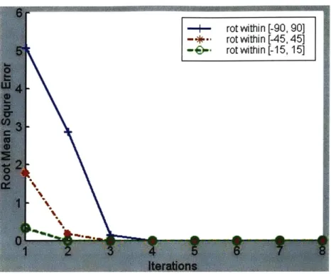
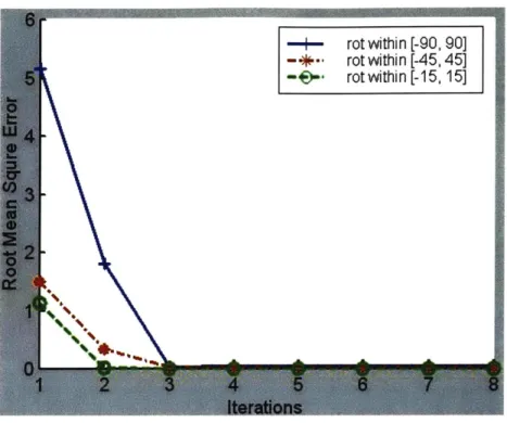
2.3.1 W ide range of rotation angles a... 38
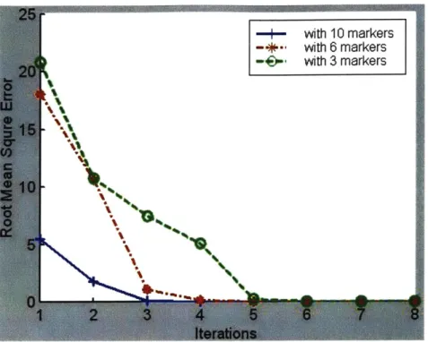
2.3.3 N um ber of m arkers ... 41
2.4 Sum m ary ... 42
CHAPTER 3 RECONSTRUCTION FROM TWO IMAGES... 43
3.1 Introduction... 43
3.2 Geom etry of the Im aging System ... 44
3.3 D escription of M ethod ... 46
3.3.1 Feature representation... 46
3.3.2 Stereo m atching ... 49
3.3.3 D isparity refinem ent ... 51
3.3.4 H ierarchical coarse-to-fine strategy... 52
3.4 Experim ent and Results ... 54
3.5 D iscussion and Conclusion... 57
CHAPTER 4 RECONSTRUCTION FROM MULTIPLE IMAGES... 59
4.1 Introduction... 59
4.1.1 Related Work... 60
4.1.2 Overview ... 62
4.2 D escription of M ethod ... 63
4.2.1 M oving Stereo Reconstruction... 63
4.2.2 Integration Process... 72
4.3 Experim ent and Results ... 76
4.3.1 Reconstruction Result ... 79
4.3.2 N um ber of Im ages ... 83
4.4 D iscussion and Conclusion... 84
CHAPTER 5 DISCRETE TOMOGRAPHY... 87
5.1 Introduction and Overview ... 88
5.2 Review of Statistical Reconstruction ... 91
5.3 D escription of M ethod ... 93
5.3.1 N otations ... 93
5.2.3 EM Algorithm Development ... 98
5.3.4 An Efficient Algorithm for Linear Equation ... 100
5.4 Algorithm Implementation... 102
5.4.1 A Priori Probability Model... 102
5 .4 .2 In itia liza tio n ... 1 04 5.4.3 Estimation of Unknown Class Values... 104
5.5 E xperim ent and R esults ... 105
5.6 Discussion and Conclusion... 107
CHAPTER 6 CONCLUSIONS AND FUTURE DIRECTIONS ... 109
APPENDIX A JAVA GUI PROGRAM FOR IMAGE PAIR ALIGNMENT AND RECONSTRUCTION ... 111
A . 1 A lignm ent Program ... 111
A.2 Manual Stereo Reconstruction Program ... 114
APPENDIX B STATISTICAL MEASUREMENTS OF CELLS CHARACTERISTICS... 116
B. 1 Cell Alignment Direction and Eccentricity... 116
B.2 Probability Function Estimation... 117
B .3 E xperim ent and R esults... 118
B .4 C o n clu sion s ... 12 0 REFERENCES... 121
List
of Figures
Figure 1 An example of cell cytoskeleton image from electron microscope ... 11
Figure 2 Parallel axis stereo geom etry... 14
Figure 3 Projection imaging geometry of tomography... 16
Figure 4 Duality relationships between algebraic method and direct method... 20
Figure 5 Performance on different range of rotation angles ... 39
Figure 6 Performance on imperfect tilt angles... 40
Figure 7 Performance on different number of marker points ... 42
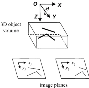
Figure 8 Geom etry of the im aging system ... 45
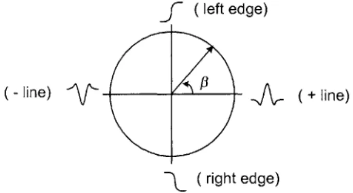
Figure 9 A representation of the local phase P as a complex vector ... 48
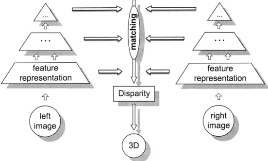
Figure 10 Hierarchical architecture of the computation ... 53
Figure 11 Example of electron microscope stereo images (400x400 in pixels) of cell cytoskeleton which were taken at ±100 of tilt angles: (a) left image; (b) scale bar; (c) right image. The reconstruction is performed on the region indicated by the white box (320x240 in pixels)... 55
Figure 12 Reconstructed 3D cytoskeleton structure visualized by isosurface method... 56
Figure 13 Procedures of the reconstruction from multiple images... 63
Figure 14 The image sequence is obtained by a rotational motion... 65
Figure 15 Projection and backprojection of an object point ... 66
Figure 16 Illustration of the generation of the correlation between two images ... 70
Figure 17 Different-valued objects have different-valued projections in the image ... 75
Figure 18 Selected cell cytoskeleton images taken on IVEM ... 79
Figure 19 The Z-slices of the reconstructed volume with 22 images ... 82
Figure 20 Visualization of the reconstructed volume by ray-casting method ... 82
Figure 21 The quality improves as more images are used for reconstruction. ... 84
Figure 22 A binary lattice and its row and column projections... 89
Figure 24 A synthetic discrete-valued phantom ... 106
Figure 25 Reconstruction and comparison: (a,b,c) reconstructions using filtered backprojection (FBP) from projections of 10, 20, 30, respectively; (d,e,f) reconstructions done by our algorithm from projections of 10, 20, 30, respectively. ... 1 0 6 Figure 26 RMSE measure of reconstructions by proposed algorithm and FEB method 107 Figure A. 1 Screen shot of GUI for alignment program... 112
Figure A . 2 a screen shot of anim ation window ... 113
Figure A. 3 a screen shot of stereo reconstruction program ... 114
Figure A. 4 a screen shot of 3D visualization window ... 115
Figure B. 1 The cells exhibit the morphological changes under different conditions: (a) situation A without fluid shear stress and (b) situation B with extem fluid shear stre s s ... 1 1 9 Figure B. 2 Probability distribution function of cell directions: (a) no dominant direction in situation A; (b) dominant direction is 30.00 in situation B. (red line is estimated prob ability function .) ... 119
Figure B. 3 Probability distribution functions of cell size measured in length of major and minor axes: (a) ratio estimation is about 1.04 in situation A; (b) ratio estimation is about 1.86 in situation B. (red line is estimated probability function.) ... 120
This thesis is intended to summarize the research in which I have participated over the past four and half years. The goal of my project mainly aims to explore and develop a new technique that is capable of reconstructing structural information from 2D electron microscope images and furthermore to provide quantitative measurements about some biological structures, e.g., the cell cytoskeleton. This Chapter gives an overview of the thesis and some background that this thesis will rely on.
1.1 Origin of Research
The motivation of this project originated from the need to obtain 3D cellular structural properties in our studies of cell cytoskeleton. The cytoskeleton of eucaryotic cells is primarily composed of three types of polymers: actin filaments, microtubules and intermediate filaments. Actin filaments are the most abundant components and they are arranged into a 3D structural network that gives the cytoplasm its shape, form, and mechanical properties. Considerable effort has gone into defining the structural and biochemical properties of the 3D polymer systems that comprise the cytoskeleton. One technique that has been widely applied to understanding this architecture is electron microscopy (EM). Figure 1 exhibits an example of cell cytoskeleton image. The images (or micrographs) taken from EM provide information on the length, geometry, and interaction and location of various cytoskeletal components. However, the images are only a 2D representation of 3D objects. Structural studies are often hampered by the inability to faithfully obtain the complicated 3D geometric relationships made by actin filaments as they course throughout the cytoplasmic space. Over the past years, 3D information is obtained largely by manual measurements. Not only is such manual work
tedious, but also the measurements are very subjective and inaccurate. Therefore, it is very desirable to develop a compute-automated system that reconstructs the 3D structures from 2D images by computer and ultimately makes the measurements on the reconstructed structures. The thesis will mainly focus on the first part of the problem, i.e., the reconstruction of 3D structures from given 2D images.
Figure 1 An example of cell cytoskeleton image from electron microscope
1.2 The World of 3D Reconstruction
3D reconstruction from 2D images in general has been of interest in a number of fields, including computer vision, robotics, medical imaging, structural biology, etc. The methods used for 3D reconstruction can roughly be categorized into two groups: one is a computer vision approach and the other is a tomographic approach. This separation is mainly due to their different treatments of the imaging function. The imaging function is defined as a function that maps the relationship between image and object. It describes how the brightness or intensity value in the image is related to the object value or some property value of the object in 3D space. The tomographic approach focuses on the
reconstruction in which the image records the transmission or emission property of the object. The imaging function is relatively simple. For instance, in linear tomography, the value in the image is represented as the integral of the object's property values along the imaging direction. On the other hand, the computer vision approach often deals with the reconstruction problem in which the image primarily describes the reflectance of the object, e.g. an image taken by a camera. The related imaging function is usually very complicated, which may involve the object's shape, its reflectance properties, position,
and illumination.
1.2.1 Computer Vision
Computer vision has emerged over the years as a discipline that attempts to enable the machine or computer to sense and interact with the environment. Major efforts have been directed towards the reconstruction of 3D structure of objects using machine analysis of images (Dhond and Aggarwal 1989). However, unlike the tomographic reconstruction, there is no mathematically sound inverse reconstruction method. This is mainly because computer vision has much more complicated relationship between image and object than tomography does. This complexity involves the object's shape, its reflectance properties, position, light sources, etc. The imaging function is sometimes very difficult to obtain.
In computer vision, the understanding of 3D structure is primarily extracted from the geometric relationships between images (Grimson 1980; Grimson 1985; Dhond and Aggarwal 1989; Faugeras 1993; Okutomi and Kanada 1993; Kanada and Okutomi 1994). The images of a 3D object are typically taken at the different locations. The positions of the object in the images are therefore different. This difference, termed disparity, is directly related to the position of the object in 3D space. In other words, the 3D information about the object is embedded in the images in the form of disparity. For instance, Figure 2 illustrates a famous stereo vision model of parallel axis geometry. The camera is simply represented by a pin-hole model. Let us denote (X,Y,Z) as a point on an object in 3D world coordinates with origin at 0. Its positions in two images are denoted by (xi, y') and (Xr, yr) with respect to their own image coordinate system. Letf be the focal
length of both cameras and d be the baseline distance between two camera. By simple triangulation, we have x1 X+d12x 1 X~d/2(1.1) f Z Xr -X-d/2 (1.2) f Z -- -r - (1.3) f f Z
Solving for (X,Y,Z) gives:
X d(x, + Xr) (1.4) 2(x -Xr) Y= d(y,+ Yr) (1.5) 2(x,- x,) Z= df (1.6) (x1 -xr)
where (xr-xr) in the equations are often referred as the disparity. The equations indicate that if we know the object's projection positions in two images, we can fully determine the object position in 3D space. The implication is very powerful. The reconstruction problem is therefore simplified to find the object's projection positions in images. However, finding the corresponding projection position in images, called matching, is usually not trivial. Over the years, a number of matching techniques have been developed. We will discuss them in details in Chapter 3. Also in Chapter 3, we will study a different type of imaging model that results in a completely different set of equations but the concept remains the same.
One of the advantages of this reconstruction method is that we don't need to worry about the complicated imaging function between the image and the object. The reconstruction can be applicable to any type of imaging systems. However, since no imaging function is used, the exact values of the object cannot be obtained. The obtained reconstruction only provides the locations or the shapes of the 3D object. In other words, we may only tell whether there exists an object or not. We cannot know what value the object may take.
The tomographic reconstruction that will be discussed later is completely different in this point. It can give both location of the object and the value of the object because the reconstruction is derived from the given imaging function.
(XYYZ)
(X1 ,(X
Left Right
Camera Cm
Figure 2 Parallel axis stereo geometry
Besides the reconstruction from disparity, there are several other 3D reconstruction techniques in computer vision. For example, shape from shading (Horn 1986; Horn and Brooks 1989), which requires a manageable imaging function, reconstructs 3D surface from 2D images with different shades. The technique is based on the observation that under different illumination conditions the image brightness responds differently based on the surface orientations. There have been some successful stories of this technique but its use is still very limited because controlling illumination condition and surface properties are practically very difficult. Interested readers are referred to related literature (Horn 1986; Horn and Brooks 1989). Another alternative reconstruction method in computer vision is optical flow (Horn 1986). Optical flow provides a reliable approximation to the image motion. Barron et al (Barron, Fleet et al. 1994) did a very good review on various optical flow algorithms and their performances. Optical flow can be used to estimate the disparity map between images. With disparity map, 3D surface or object may be recovered via geometric relationships such as Equations (1.4) ~ (1.6). This two-step procedure is often referred as indirect method. In contrast, Horn and Weldon (Horn and Weldon 1988) developed a direct method for scene reconstruction using
optical flow. Shashua and Stein (Shashua 1995; Stein and Shashua 1996; Stein 1998; Stein and Shashua 2000) further expanded the approach to three views. In both the direct and the indirect method, the optical flow approach is based on a fundamental assumption: the constant brightness assumption. It assumes that the brightness pattern of the object remains the same between images even though their positions may change. In order for this assumption to be applicable, there are some strict requirements, such as Lambertian surface, uniform illumination, etc. These conditions are normally hard to satisfy in practice.
As a summary, due to the complexity of the imaging function in computer vision, there is no direct inverse reconstruction from the image to 3D object. The reconstruction is primarily obtained by establishing the geometric relationship between image and object. Reconstruction from disparity is one of the most used methods in computer vision because it shields us from the complexity of the imaging function. Other methods, such as shape from shading and structure from motion (optical flow), are alternative methods of reconstruction in computer vision, applicable to some controlled conditions.
Note that in this thesis we will mainly focus on the method of the reconstruction from disparity.
1.2.2 Tomography
Tomography solves a special reconstruction problem in which the imaging function is known and has a strict form. The reconstruction can be derived mathematically via an inverse mapping function. 3D reconstruction in tomography can be considered a simple extension of the 2D tomographic reconstruction. In most situations, 3D reconstruction is obtained by stacking a series of 2D reconstructed slices. Let us begin our discussion on 2D reconstruction first.
The fundamental problem that needs to solve is the reconstruction from projections. The solution to this problem is tomography. Over the past 40 years, it has seen its rapid
developments and applications expanding into a large number of scientific, medical, and technical fields. Of all the applications, probably the greatest impact has been in the areas of diagnostic medicine (Herman 1980). It earned itself two Nobel prizes: one in 1979 for computerized tomography (CT) and the other in 1982 for electron tomography (which will be discussed separately in next subsection). In recent years, some newly emerged technologies in medicine, such as MRI (Magnetic Resonance Imaging), SPECT (Single Photon Emission Computed Tomography) and PET (Positron Emission Tomography) are all based on tomography.
x
Figure 3 Projection imaging geometry of tomography
Interestingly, as early as 1917, Radon derived mathematical theories of Radon transform and inverse Radon transform, which turned out to be the underlying fundamentals of tomography. In linear tomography, the imaging function is defined as follows: the value in each projection is the integral of the object values along projection direction. Figure 3 illustrates a 2D case of the projection geometry. The relationship is expressed as:
g(p,O)= ff(x,y)du (1.7)
U
where u is the projection direction and 5(.) is a Dirac delta function (impulse function). The projections g(p,O) can be re-organized into an image with p and 0 as two coordinates, and often called a sinogram. Therefore, the goal in tomography is to reconstruct the object functionj(xy) from its sinogram g(p,0). Equation (1.8) is actually the exact form of Radon transform. The objectJ(xy) can therefore be obtained by inverse Radon transform. Inversion of the Radon transform can be done in several ways. One standard algorithm is based on the projection-slice theorem (Mersereau 1973; Jain 1989). The theorem indicates that the one-dimensional Fourier transform of the projection g(p,0) with respect to p is equal to the central slice, at angle 0, of the two-dimensional Fourier transform of the objectf(x,y), i.e.,
G(4,0)=F,(4,O) ,(1.9)
where capital names, such as G or F, represent the function in Fourier domain and 4 is the coordinate in Fourier space. Subscript p means the variables are in the polar
coordinate system, such as Fp. If we fill the whole Fourier domain at any angle with corresponding projection, the object is then obtained by inverse Fourier transform. Mathematically, it can be derived as follows (Jain 1989; Toft 1996). The inverse Fourier transform is given by:
f(x, y) = f f F(,, 4,) exp [j2 (4,x + ,y)] d4,d (1.10) -00 -00
When written in polar coordinates in Fourier domain, Equation (1.10) gives:
f (x, y) =f F(4, 0)exp
[j27r
(x cos0 + y sin0 )] d4 d(1.11) fJf G(4,0) exp[j22r4(x cos0 + y sin0)]d4dA
= g(x cos0 + y sin 0,0)d0 , (1.12)
0
where
Equation (1.13) is an inverse Fourier transform of function |4IG(4, 0), which can be considered a filtered version of G(4, 0) with the high-pass filter 1
I
in Fourier domain. Equation (1.12) is called back-projection. In fact, these two equations, Equations (1.12) and (1.13) form the famous filtered-backprojection (FBP) method, which involves two steps. First, each projection g(p,0) is filtered by the one-dimensional filter whose Fourier transform is |4| (which is Equation (1.13)). The result, g(p,0), is then back-projected to yieldJ(x,y) (which is Equation (1.12)).It is also possible to make the backprojection before the filtering (Herman 1980; Jain 1989). The method is called filtering after backprojection (FABP), as well as rho-filtered layergram in some early literature. In this method, a different filter must be used. The procedures are given as follows:
7r
f(x, y) = g(x cos0 + y sin0,0)dO (1.14)
0
f (x, y ) =
J(,,
+ ) exp(j2)T
(4xx + y ) dCxd4, (1.15)-00 -00
where F(4,, ,) is the Fourier transform of f(x, y). The filter is a two-dimensional filter with the form of 4 + in Fourier domain. Although FABP method is not used as popularly as FBP method in practice, it achieves comparable performance to FBP (Suzuki and Yamaguchi 1988). In Chapter 5 of the thesis, we will come back to FABP method which helped us to derive an efficient algorithm for discrete tomography. One common property of both FBP and FABP methods, as indicated in Equation (1.12) or (1.14), is that they require a full range of projections (0 from 0 to 7r). The incomplete projections may lead to incorrect reconstruction.
In practice, perfect reconstruction described by the above methods can not be achieved because we cannot obtain an infinite number of projections for the integral operation in Equations (1.12) and (1.14). Furthermore, the methods have to be implemented in the computer and all operations are approximated by their discrete versions. Therefore, each
method has its reconstruction limit. The resolution is typically dependant on the angle between adjacent projections (AO) and the point resolution in each projection (Ap).
Besides the direct inverse formulas above, inversion of the Radon transform can also be obtained via some iterative methods, such as algebraic reconstruction techniques (ART) (Gordon, Bender et al. 1970) or expectation maximization (EM) methods (Shepp and Vardi 1982; Green 1990). In comparison to the direct reconstruction method, iterative methods are usually very expensive in computation. However, they may achieve better reconstruction quality. More importantly, iterative methods offer a great deal of flexibility and robustness. They can deal with situations like incomplete projection data, uneven-sampled projections, noise-deteriorated projections, reconstruction with constraints, etc. None of the direct inverse methods can easily handle these common but difficult situations. It is because of these advantages that iterative methods have gained a lot of attention and popularity in many medical applications, such as PET and SPECT. We will review some of the well-known iterative reconstruction techniques later in the thesis. Those iterative methods form the basis to our algorithm for discrete tomographic reconstruction.
One important observation worthy of mentioning is the duality between linear algebraic operations and the Radon / inverse Radon transforms. In discrete implementation, the linear projection of Equation (1.7) can be represented by the sum of the object points along the projection path. If we represent the all object points in a vector form denoted by x and all projection points in a vector form denoted by b, the projections can then be written in a matrix vector formulation:
b = Ax (1.16)
where A is coefficient matrix containing the weighting factors between each of object points and projection direction. With this linear algebra formula, the reconstruction problem becomes to solve the linear equation of Equation (1.16). Since matrix A is non-square, one approach to solve Equation (1.16) is to form a normal equation:
ATb = A
where AT is the transpose of A, and ATA is a square matrix. If we assume A A is invertible, the solution of the linear equation is given by:
x = (ATA)-'Ab. (1.18)
Let us draw some analogy between this linear algebraic form and the direct inverse Radon transform (Kawata and Nalcioglu 1985; Toft 1996). Equation (1.16) corresponds to the Radon transform, which does the forward projection. Thus, Equation (1.18) essentially represents the inverse Radon transform. More interestingly, if matrix A is considered a projection operator, its transpose A is actually a backprojection operator. Therefore, Equation (1.18) can be interpreted as filtering after backprojection (FABP) with A representing backprojection and (ATA)l representing the filter. This filter corresponds to the one given in Equation (1.15). Similarly, filtered backprojection (FBP) can be matched to a different form of linear equation solution:
x = (ATA)-1ATb (1.19)
= (A T A)-1 AT (AAT )(AA T )-' b = A T (AA T )-'b .(1.20)
In Equation (1.20), (AAT)l corresponds to the high-pass filter in Equation (1.13). The backprojection AT is performed after filtering. In summary, Figure 4 lists these duality mappings. Ax = b A A T x = A T (AA T )-1b (AAT )y x = (A T A)-' AT b (A T A)-1 b is projection projection operator backprojection operator FBP method filter in FBP method FABP method
filter in FABP method Figure 4 Duality relationships between algebraic method and direct method
So far, the reconstruction from projections has been focused on 2D tomography. 3D reconstruction can simply be constructed from 2D case slice by slice. Alternatively, 3D
_4MO ~p _4M 0 _OM 1 _OWKZ -OMMEMBOO _O=M=8O _OMMEMP-@
tomography can also be obtained by 3D Radon transform and inverse 3D Radon transform (Deans 1993). Both direct inverse and iterative methods are applicable in 3D but may have a different form. Some types of 3D projection and reconstruction are
described in (Toft 1996).
1.2.3 Electron Tomography
Electron tomography specifically refers to the technique that employs an electron microscope to collect projections of an object and uses these projections to reconstruct the object (Frank 1996). It inherits all the theories developed in tomography. In structural biology, it is currently the primary approach of 3D reconstruction for macromolecular or sub-cellular level structures, such as virus or ribosome (Frank 1996). In some literature, one would prefer to exclude crystallographic methods from electron tomography, more or less for historical reasons. Crystallography specifically refers to the technique that makes use of inherent order or symmetry properties of the object in reconstruction (DeRosier and Klug 1968). Electron tomography is considered a more general theory of reconstruction that makes no assumption of the presence of the order or symmetry. Fundamentally, both crystallography and electron tomography are based on the same underlying theorem: the projection-slice theorem, developed in tomography. The goal of the reconstruction is to use projections to fill the entire Fourier space as the theorem suggests.
Unlike the tomography in medical applications, electron tomography faces a number of its own obstacles. The first is the restricted tilt angles of the electron microscope. The angular range in most electron microscopes does not exceed ±600. A significant portion of the Fourier transform is simply missing, which may result in a great deal of distortion in the reconstruction. However, crystallography is one exception. Because of the symmetries, crystallography has been very successful in dealing with this issue when reconstructing crystalline objects. Due to the same symmetries in Fourier space, the missing part of the Fourier transform can be inferred and derived from other parts of the Fourier space and the entire Fourier transform can therefore be obtained. Another special
case is some macromolecules that exist structurally identical copies in the volume considered. These identical copies typically have random orientations in each projection. The projection copies at these orientations can be used to make up the missing projection at unreachable tilt angles. Therefore, the missing part of Fourier transform can be filled as well. The current applications of Electron tomography have primarily focused on these macromolecular structures (Frank 1992; Frank 1995). However, in nature, the biological structures or entities that fit these special criteria are very limited. The development of electron tomography has been hampered greatly because of this.
The second obstacle is the strict imaging function requirement. Since both tomography and electron tomography are based on projection-slice theorem. The applicability of the theorem relies on the imaging relationship between projection and object being the form of Equation (1.7). In the case of electron-microscope imaging system, such relationship usually doesn't hold well. Some approximation has to be made. The condition for approximation is dependant on the specimen preparation, imaging conditions, etc. (Frank 1992)
Another issue is the difficulty of preserving the native structure during specimen preparation and image collection. The associated problems are two folds. One is the ability of the electron beam to penetrate the specimen. The second is the structural damages induced by multiple exposure to electron beams during imaging. The former one tends to suggest the use of intermediate to high voltage electron microscope while the latter one suggests the opposite. In addition, in order to improve the contrast, the specimen is often carefully stained or gold-labeled (Hartwig 1992; Frank 1996). However, the presence of heavy atoms in stained specimen makes the approximation of the imaging function untenable.
Notwithstanding these obstacles, electron tomographic techniques have had tremendous success and impact in structural biology. In recent years, many new developments have been witnessed. For instance, the technique of double-tilt is used to reduce the size of the angular gap (Penczek, Marko et al. 1995). However, obstacles still exist. Electron
tomography is still not generally applicable to a large number of biological structures or entities. The thesis, in some ways, attempts to explore an alternative reconstruction technique that would tackle some of these obstacles.
1.3 Bayesian Estimation
Let us look at the reconstruction problem from a different perspective. The central problem of reconstruction is to recover the object from its projections. It perfectly fits into the estimation methodology where we want to estimate the unknown input (the object) from the given output (the projections). Estimation of input from output has been a very classical problem in many areas. In statistic estimation, the problem can be approached by attempting to answer this question: what is the statistically best input that generates the given output?
In this section, we will first briefly introduce some mathematics and terminology of statistical estimation. Focus will be on discussing estimation methods under a Bayesian framework. We assume that readers are familiar with basic probability and statistics, such as random variables, random vectors, probability function, mean, variance, etc. In the thesis, a prevailing convention is adopted: probability distribution function P(.) (capital letter P) is used when the considered random variable is discrete, and probability density function p(.) (low-case letter p) is used when the random variable is continuous. Bold case is used to refer a random vector, such as x, while non-bold represents a scalar random variable, such as x.
1.3.1 Conditional Probability and Bayes' Rule
We will frequently deal with several random variables. These random variables may or may not be related to each other. If they are, we hope that they may be predictable from each other. However, the predictability is not guaranteed. For instance, when two random variables are completely independent, knowing one random variable does not help to
The relationship between random variables can be characterized by the joint distribution and conditional distribution. The joint distribution of two random variables, P(XY), describes the co-occurrence of both events X and Y. The marginal distribution, which defines the occurrence of either X or Y, can be obtained from their joint distribution:
P(X) = Z P(X, Y = y) (1.21)
P(Y) = Y P(X = x,Y ) (1.22)
XEQX~
where Qx and Q y are sample spaces of random variable X and Y, respectively.
The conditional distribution, P(XY), describes the probability of random variable X given
Y. It is defined as:
P(X I Y)P(XY) . (1.23)
P(Y)
Likewise, the conditional distribution, P(X), is given by:
P(Y X) P(XY) . (1.24)
P(X)
A straightforward extension of Equations (1.23) and (1.24) is the well-known Bayes' Rule, which inverts the conditional distributions:
P(Y I X)P(X)
P(X
I
Y) = .P() (1.25)P(Y )
When random variables are continuous variables, similar definitions are given to the probability density functions. In brief, the marginal density functions are obtained from:
P"(x) = fP,,(x, y)dy (1.26)
PY= (f p,,(x, y)dx. (1.27)
The relationship between joint density function and conditional density functions are given by:
Therefore, Bayes' Rule is easily derived from Equation (1.28): p)I (y Ix)p, (x)
px y I(Y = = p (x) .x (1.29)
p,(y)
Bayes' Rule has been very useful in decision theory, estimation, learning, pattern classification, etc. For instance, in estimation problem, Equation (1.29) can be used to find the best estimation of unknown variable x from given observations of known variable y.
Finally, we would like to stress that the above definitions and derivations hold not only for random variables but also for random vectors.
1.3.2 Bayesian Estimation Methods
In the Bayesian framework, we refer to the probability density px(x) for the vector x to be estimated as the a priori density. This is because this density fully specifies our knowledge about x prior to any observation of the measurement y. The conditional density py (yx), which fully specifies how y contains the information about x, is typically called the likelihood function. Generally, this likelihood function, pyw(ylx), is not directly given but can be inferred from the measurement model. The conditional density pxL(xLy) is called the a posteriori density because it specifies the behavior of x in accordance to the measurement y.
We refer to the estimation of x as the estimator denoted by k. Let X (y) denote the estimation of x based on measurements y. In a Bayesian framework, we choose the estimator so that it optimizes some performance criterion. For instance, a cost function
C(x, x) is often used to evaluate the cost of estimating an arbitrary vector x as .Ci. The
best estimator is defined as the one that minimizes the average cost given y:
x(y) = arg min EC(x,a) y] a
(1.30) = arg min C(x, a)pxly (x y)dx
As Equation (1.30) indicates, the a posteriori density function plays an important role in Bayesian estimation.
Consider the cost function given by:
1 1 a - a 1> e
C(a,a)= 0 otherwise (1.31)
which uniformly penalizes all estimation errors with magnitude bigger than E. Substitution of Equation (1.31) into Equation (1.30) gives:
^(y) = arg min(I - + 0,x| 0d
x amn
- :Pxy(x
I
y)dx](1.32) = arg max Jpxl,(x | y)dx
a
This estimator is called minimum uniform cost (MUC) estimation. It finds the interval of length 2E where the a posteriori density is the most concentrated. If we let E get sufficient small, MUC estimation essentially approaches the point corresponding to the peak of the
a posteriori density function. This is the so called maximum a posteriori (MAP)
estimation:
XMAP(Y) argmaxpX1 (a
I
y). (1.33)a
The MAP method has been one of the most widely used estimation techniques because of its simplicity and computability. The maximum of px,(xty) may be obtained by differentiating the function:
a
PI(I )=0(1.34)ax
p
I(
y) = 0.-(-4Furthermore, according to Bayes' Rule, substituting Equation (1.29) into Equation (1.34) leads to:
r
px(ylx)px(x) (1.35)ax p,(y)
9
Since py(y) is not a function of x, Equation is equivalent to
It is sometimes more convenient to maximize some monotonic function of a posteriori density than itself. For example, a normal log function is often used. Maximizing lnps,(x[y) is often easier than maximizing pxy(x y) directly. In this case, the MAP equation of (1.36) is rewritten as:
a
a
--In p,(y I x) + - In px (x) = 0 . (1.37)
ax ax
Equation (1.37) indicates that MAP estimation is only dependent on a priori density px(x) of x and likelihood function py jyx).
Let us consider a rather special case. If our knowledge indicates that x is only an
unknown constant (such as some parameter), instead of a random vector, the MAP method reduces to be the maximum likelihood (ML) method. Because in this situation the a priori function px(x) becomes a constant, ML estimation can then be obtained by:
a
---In pyl(y Ix) =0. (1.38)
ax
This illustrates the close relationship between ML and MAP methods. A formal derivation of ML estimation can be found in any good book on statistics (Papoulis 1991).
As a final remark, with a different cost function, we may achieve many other estimation methods, such as minimum absolute-error (MAE) estimation, minimum mean square error (MMSE) estimation, etc. Choosing a suitable method for a particular problem depends on a variety of factors, including the knowledge about the unknown x and
observation y, the importance of errors, the computability of optimization, etc.
1.3.3 Markov Random Field (MRF)
A priori information about x is very important and useful in estimating x. Intuitively, the
more a priori information we know about x, the better estimation we can expect to
obtain. In addition, as Equation (1.37) indicates, knowing the exact form of the a priori
function is necessary for MAP method to be applied. In many problems, the a priori
MRF defines a field of random variables whose relationships are represented by a neighborhood structure. In discrete case, the field is often represented by a lattice, composed of a set of sites or nodes in a graph. For example, an mxn image can be represented as an mxn lattice where each site corresponds to a pixel in the image. One of the most important properties of MRF is local characteristics, which asserts conditional independence: given its immediate neighbors, a random variable of MRF is independent of all other variables. Mathematically, this property is expressed by:
P(x, I x, Vr # s) = P(x, I x, VrE Ns) (1.39) where s (a site) represent a variable under consideration and N, is its neighborhood. The left-hand side of Equation (1.39) is the conditional probability of the variable given the rest of other variables in the lattice. The right-hand side of Equation (1.39) is the conditional probability of that variable given the states of all variables in its neighborhood. The neighborhood N, is defined as a collection of "neighbors" of the site
s. Neighbors are dependent on the order of the neighborhood to be considered. For
instance, a first-order neighborhood of a pixel (i, j) in an image is composed of pixels immediately above, below, to the left and to the right of the given pixel (ij), i.e.,
NY={(i-1, ), (i, j-1), (i, j+1), (i+1, j)}. A second-order neighborhood includes the first order
neighbors as well as pixels that are diagonally across from the given pixel, i.e., NU={(i-1,
j), (i, j-1), (i, j+1), (i+1, j), (i-1, j-1), (i-1, j+1), (i+1, j-1), (i+1, j+1)}. Higher order
neighborhood can be similarly defined, but they are rarely used in practical applications. Let us introduce another term, clique. A clique c is defined as a subset of sites in S (the space of s) and neighborhood N (Li 1995). It consists either of a single site c={s}, or of a pair of neighboring sites c= {s, s'}, or of a triple of neighboring sites c= {s, s', s "}, and so
on. The collections of single-site, pair-site and triple-site cliques are denoted by C1, C2, C3, respectively:
C, = {s Is e S}
C2={{s,s'}Is e S,s'e
N,}
C2 = {{s, s', s "}Is, s', s " e S are neighbors to each other} .
(1.40) (1.41)
(1.42)
C = C, U C2U C( 1.43
The Hammersley-Clifford theorem provides us a systematic way for modeling MRF (Besag 1974; Geman and Geman 1984; Besag 1986; Li 1995). The theorem establishes equivalence between MRF and Gibbs random fields (GRF) and allows us to construct MRF using a GRF model. With this equivalence, the conditional distribution model of MRF is converted to a joint distribution model of GRF. The Gibbs distribution is given as:
P(x) = Iexp(- E(x) , (1.44)
Z T
where T is a constant called the temperature. Z is a normalizing constant, Exx
Z = Iexp(- E() (1.45)
X T
and also known as partition function. It ensures that the sum of all probabilities P(x) is equal to 1. E(x) is called the energy function and expressed as a sum of clique potentials over all possible cliques C:
E(x) = IV, (x) . (1.46)
eC
The value of Ve(x) depends on local configuration on the clique c.
In recent years, MRF has been of great interests in many areas, such as computer vision and image processing (Geman and Geman 1984; Geiger and Girosi 1991; Kapur, Grimson et al. 1998). It works particularly well when a problem involves uncertainties or constraints that are difficult to solve by other methods. MRF offers a great deal of flexibility for modeling different types of a priori information, such as local smoothness (Geman and Geman 1984; Geiger and Girosi 1991), geometric relationship (Kapur, Grimson et al. 1998), etc.
1.4 Overview and Contributions
Due to limitations of electron microscopy, a lot of biological structures can not be reconstructed directly by electron tomography. Furthermore, when a specimen is stained with heavy metals, the imaging function no longer satisfies the condition of the projection-slice theorem. Tomographic reconstruction methods won't work well in these situations. This thesis attempts to explore and develop a new reconstruction technique that can be applied to a large variety of structures, especially to ones that are intractable using electron tomography. It may serve as an alternative method to electron tomography in structural biology.
This thesis addresses reconstruction problems in a more general context, covering both computer vision based reconstruction and tomographic reconstruction. However, specific attention is given to 3D reconstruction of biological cellular structures, such as cell cytoskeleton, from electron microscope images taken at different tilt angles. The thesis is composed of two parts. At the first part of the thesis, we study reconstruction from a computer vision perspective. As mentioned earlier, the reconstruction by computer vision approaches doesn't require exact knowledge of an imaging function, and 3D information is extracted mainly from the geometric relationship between images. This shields us from complexity of the imaging function. Interestingly, computer vision based reconstruction has rarely been used in biological applications. As one of our goals, we hope that this thesis will bring computer vision based techniques to the attention of structural biology communities.
We first derive the geometric relationship that describes the imaging system of electron microscope. Then, the thesis focuses on finding structural relationships between 3D objects and 2D images. Based on a stereo vision idea, a stereo reconstruction method is presented, which reconstructs 3D structure from only two images taken at two different tilt angles. A multiple-feature matching algorithm is employed. The algorithm introduces a complex-value representation that takes into account both feature value and the certainty of this value. A volumetric reconstruction method is then developed by
extending stereo reconstruction to reconstruction from multiple images. The method integrates a sequence of 3D reconstruction from different image pair. The integration is an optimization process that attempts to find the best estimation for each location in a 3D object space. As an example of applications to biological structure, the proposed approach is tuned and applied to 3D reconstruction of cell cytoskeleton structure from multiple images taken at different tilt angles on an electron microscope. The reconstruction demonstrates the feasibility, reliability and flexibility of the proposed approach.
The second part of this thesis focuses on a special tomographic reconstruction, namely discrete tomography. Discrete tomography deals with a reconstruction problem in which the object to be reconstructed is composed of a discrete set of materials each with uniform values. Such condition or constraint is termed discreteness in this thesis. The discreteness can be confirmed from observations that each type of biological structure tends to have one uniform value in its electron microscopy images.
Discrete tomography has recently been of interest to many fields, such as medical imaging (Frese, Bouman et al. 1998; Vardi and Lee 1998; Chan, Herman et al. 1999; Herman and Kuba 1999). This thesis studies discrete tomography in a general format. The proposed approach starts with an explicit model of the discreteness constraint. within a Bayesian framework. The problem of discrete tomography is converted into a Bayesian labeling process, assigning a unique label to each object point. The formula also establishes a mathematical relationship between discrete tomography and conventional tomography, suggesting that discrete tomography may be a more generalized form of tomography and conventional tomography is only a special case of such generalization. An expectation-maximization (EM) algorithm is developed to solve discrete tomography. An efficient solution for discrete tomography is proposed in the light of the duality of tomographic reconstruction methods discussed in earlier section.
As a summary, this thesis studies 3D reconstruction from 2D images using imaging function as guidance. The thesis is primarily composed of two parts that corresponds to
two different treatments to the imaging function. In the first part of thesis, a computer vision based reconstruction is developed, which doesn't require any knowledge of the imaging function. The second part of thesis deals with discrete tomography in which an approximation of the imaging function is used and some constraints are considered.
The key contributions of this thesis are closely related to these two parts as well:
. The thesis develops computer vision based reconstruction methods for both stereo images and multiple images. The proposed volumetric reconstruction method can be applied to a large number of biological structures, demonstrated by the reconstruction of the cell cytoskeleton from multiple images. The approach offers an alternative reconstruction technique to electron tomography in structural biology.
. The thesis proposes an integrated model for discrete tomography and develops a Bayesian labeling method and an efficient algorithm. A mathematical relationship between discrete tomography and conventional tomography is established and
2.1 Overview
As described in the previous Chapter, 3D information of objects is embedded within 2D images in the form of disparities. For instance, 3D positions can be recovered by triangulation from the disparities among 2D images (Marr and Poggio 1979; Grimson 1980; Grimson 1985). However, due to inherent deviations of imaging device or movements introduced during image acquisition process, images obtained are rarely in perfect alignment with respect to each other. Disparities among images are often contaminated and contain in-plane translations, rotations, and/or even scaling change of each image with respect to the other. The alignment is a process that compensates these movements so that the images will share a common coordinate system and the disparities will truly reflect 3D information of the objects. The alignment is a necessary pre-process
before reconstruction can be conducted.
The fiducial-marker alignment method, developed by Lawrence (Luther, Lawrence et al. 1988; Lawrence 1992), is used widely in electron tomography field. It requires users to manually pick several markers from each image. In biological applications, markers are often made by embedding gold particles into specimen before taking images. Image movements, including in-plane translation, rotation and scaling, are then calculated by minimizing a least-square error between measured marker coordinates in images and their true coordinates projected from 3D space. However, this least-mean-square-error (LMSE) method results in a set of non-linear equations. Solving these non-linear equations is often computationally difficult and time-consuming.
In this Chapter, we propose a new and iterative algorithm with which the solutions for alignment can be obtained from a set of linear equations, as opposed to non-linear ones. The proposed algorithm proves to be fast and robust.
2.2 Iterative Algorithm
The proposed algorithm also adopts the idea of using fiducial-markers. Markers need to be picked manually in each image. The number of markers needed can be as few as two in each image. However, more markers improve accuracy and quality of the alignment. We have developed a graphic user interface (GUI) program to help users with this process. The program is described in Appendix A. In addition, since electron microscope imaging system is modeled by parallel projection, the scaling factor is negligible. Thus, only in-plane translations and rotations need to be computed in the alignment.
Let us assume markers have been picked from each image and denoted by (xij, yij), where
(x, y) is the coordinate in each image plane. Let i=1,2,..,m denote the ith image plane with
corresponding tilt angle 0, .Let j=1,2,...,n denote the jth marker. Denote XYZ as the common 3D coordinate reference frame where 3D objects are imaged. With a parallel projection model, the geometric relationship of a point's position in 3D space and its coordinates in the image plane is given as follows:
x,4 = Ri P T Xi + di , (i = 1, 2,..., m ; j= 1, 2,..., ) (2.1)
where xij is the image coordinate vector [Xij, yj] T (where T represents transpose) of the projection of thejth marker in the ith image plane, where T represents transpose. X1 is the
position vector [X, Y Zj] Tfthejth marker in the 3D common coordinate system. Ti is ao, 3x3 rotation matrix representing the tilting operation with tilt angle 0i. P is a 2x3 projection matrix. R is a 2x2 rotation matrix describing the in-plane rotation of the ith image plane with angle ai. d, is a two-dimensional vector representing the in-plane translation of the ith image plane. Let us assume the tilting axis is always the Y-axis and parallel to image planes. The transformation matrices in Equation (2.1) have this form:
cos 0 0 --sinO
1
-Ti 0 1 0 0 [cosai -sinai
Ti=
I0
1 0I,
P=I , Ri=I'I.
(2.2)sin 0 cos
]
L0 1 0- Cosa]There is one very important observation from Equation (2.1): the common coordinate system is translation-invariant. It means that if the common coordinate system is translated, we can always find in-plane translations di such that the image coordinates xij remains the same. Therefore, the in-plane translations di are merely relative values with respect to the common coordinate system we choose. This property holds mainly because of the parallel projection model of our imaging system.
Bearing this property in mind, let us proceed to solve the alignment. The alignment can be considered to solve an inverse estimation problem. It seeks to retrieve unknown inputs
X, and the best set of parameters, Ri 's and di 's, from known output markers' position xij
in each image plane. The LMS method is adopted to minimize the mean square error (MSE) between the measured marker coordinates in the images and their true coordinates projected from the 3D space:
MSE= (x R, P T X -d) . (2.3)
iij
To make the problem simpler, let us assume the tilt angle 0, 's are known and accurate. Furthermore, due to the translation-invariant property, the in-plane translations di in Equation (2.3) can be eliminated by choosing a proper reference point. It is easy to derive that such reference point is the centroid of the picked markers. Its projection in each image plane is also the centroid of the markers' projections in each image plane. They can be obtained by:
X, = , for i =2,..., m. (2.4)
n n
These reference points are then treated as the origins of the common coordinate system and each image planes. New coordinates are obtained by translations:
X'1 = Xj
-x
x. =x, -x for i =,2,..., m;j
= 1,2,...,n. (2.5)Under new coordinate systems, Equation (2.1) then becomes
X'j = R P T X'1 . (i = 1,2,..., m ; j = 1,2,..., n.) (2.6)
Unknown variables in Equation (2.6) are in-plane rotation Ri and the 3D coordinate X'; in the new common coordinate system. The corresponding MSE equation is given by:
MSE = 1 1(x' j- R P Ti X' ) . (2.7)
iij
The direct differentiation on Equation (2.7) will lead to a set of non-linear equations, which is not good for computation. However, by some manipulation of Equation (2.6), we find a linearization scheme to get around this non-linear issue. By moving the rotation matrix R, to the left hand side of Equation (2.6), a new MSE function is formed and given by:
MSE = j (R1 x' - P Tj X'1) , (2.8)
i J
where R;-1 is the inverse matrix of R;. Furthermore, let us assume the rotation angle ac is
very small for now. R can be approximated by:
cosa. s1ina
F
1 a.[-sin a cos a]
L
-a 1The LMS method on this MSE function of Equation (2.8) will then result in a set of linear equations, obtained by setting partial differentiation of ai, Xj, Yj, Zj to be zeros:
in (m
- xi + y2 i ja + (y s, - Xxi- Y + yj' Sin Oi Zj = 0 , 1, 2,..., m.
-
(y
cosO-a)+ Z cos2o + +X , Zsin =Z =cos inZ x cosOi , j=1,2,...,n.
Ki J(2.10)
in mn
Z(x 1 n) -n ( = - y , j=1,2,...,n.
- y sinO -ai)+ sin sinei-X +rsin2o -Z; = x si , , j =1,2,...,n.
This (m+3n)x(m+3n) linear equation simply has the form of: