HAL Id: hal-02969510
https://hal.archives-ouvertes.fr/hal-02969510
Submitted on 16 Oct 2020
HAL is a multi-disciplinary open access
archive for the deposit and dissemination of
sci-entific research documents, whether they are
pub-lished or not. The documents may come from
teaching and research institutions in France or
abroad, or from public or private research centers.
L’archive ouverte pluridisciplinaire HAL, est
destinée au dépôt et à la diffusion de documents
scientifiques de niveau recherche, publiés ou non,
émanant des établissements d’enseignement et de
recherche français ou étrangers, des laboratoires
publics ou privés.
Efficient Execution of Scientific Workflows in the Cloud
Through Adaptive Caching
Gaëtan Heidsieck, Daniel de Oliveira, Esther Pacitti, Christophe Pradal,
Francois Tardieu, Patrick Valduriez
To cite this version:
Gaëtan Heidsieck, Daniel de Oliveira, Esther Pacitti, Christophe Pradal, Francois Tardieu, et al..
Efficient Execution of Scientific Workflows in the Cloud Through Adaptive Caching. Transactions on
Large-Scale Data- and Knowledge-Centered Systems, Springer Berlin / Heidelberg, 2020, pp.41-66.
�10.1007/978-3-662-62271-1_2�. �hal-02969510�
Cloud through Adaptive Caching
Gaëtan Heidsieck1[0000−0003−2577−4275], Daniel de Oliveira2[0000−0001−9346−7651], Esther Pacitti1[0000−0003−1370−9943], Christophe Pradal3[0000−0002−2555−761X],
François Tardieu4[0000−0002−7287−0094], and Patrick Valduriez1[0000−0001−6506−7538]
1 Inria & LIRMM, Univ. Montpellier, France 2 Institute of Computing, UFF, Rio de Janeiro, Brazil
3 CIRAD & AGAP, Univ. Montpellier, France 4 INRAE & LEPSE, Montpellier, France
Abstract. Many scientific experiments are now carried on using scien-tific workflows, which are becoming more and more data-intensive and complex. We consider the efficient execution of such workflows in the cloud. Since it is common for workflow users to reuse other workflows or data generated by other workflows, a promising approach for efficient workflow execution is to cache intermediate data and exploit it to avoid task re-execution. In this paper, we propose an adaptive caching solution for data-intensive workflows in the cloud. Our solution is based on a new scientific workflow management architecture that automatically manages the storage and reuse of intermediate data and adapts to the variations in task execution times and output data size. We evaluated our solution by implementing it in the OpenAlea system and performing extensive experi-ments on real data with a data-intensive application in plant phenotyping. The results show that adaptive caching can yield major performance gains, e.g., up to a factor of 3.5 with 6 workflow re-executions.
Keywords: Adaptive Caching, Scientific Workflow, Cloud, Workflow Exe-cution
1
Introduction
In many scientific domains, e.g., bio-science [18], complex experiments typically require many processing or analysis steps over huge quantities of data. They can be represented as scientific workflows (SWfs), which facilitate the modeling, management and execution of computational activities linked by data depen-dencies. As the size of the data processed and the complexity of the computation keep increasing, these SWfs become data-intensive [18], thus requiring execution in a high-performance distributed and parallel environment, e.g., a large-scale virtual cluster in the cloud [17].
Most Scientific Workflow Management Systems (SWfMSs) can now execute SWfs in the cloud [23]. Some examples are Swift/T, Pegasus, SciCumulus, Kepler
2 G. Heidsieck et al.
and OpenAlea [21]. Our work is based on OpenAlea [30], which is being widely used in plant science for simulation and analysis [29].
It is common for SWf users to reuse other SWfs or data generated by other SWfs. Reusing and re-purposing SWfs allows for the user to develop new analy-ses faster [14]. Furthermore, a user may need to execute a SWf many times with different sets of parameters and input data to analyze the impact of some experi-mental step, represented as a SWf fragment, i.e., a subset of the SWf activities and dependencies. In both cases, some fragments of the SWf may be executed many times, which can be highly resource consuming and unnecessarily long. SWf re-execution can be avoided by storing the intermediate results of these SWf fragments and reusing them in later executions.
In OpenAlea, this is provided by a cache in memory, i.e. the intermediate data is simply kept in memory after the execution of a SWf. This allows for the user to visualize and analyze all the activities of a SWf without any re-computation, even with some parameter changes. Although cache in memory represents a step forward, it has some limitations, e.g., it does not scale in distributed environments and requires much memory if the SWf is data-intensive.
From a single user perspective, the reuse of the previous results can be done by storing the relevant outputs of intermediate activities (intermediate data) within the SWf. This requires the user to manually manage the caching of the results that she wants to reuse. This can be difficult as the user needs to be aware of the data size, execution time of each task, i.e., the instantiation of an activity during the execution of a SWf, or other factors that could allow deciding which data is best to be cached.
A complementary, promising approach is to reuse intermediate data pro-duced by multiple executions of the same or different SWfs. Some SWfMSs support the reuse of intermediate data, yet with some limitations. VisTrails [7] automatically makes the intermediate data persistent with the SWf definition. Using a plugin [36], VisTrails allows SWf execution in HPC environments, but does not benefit from reusing intermediate data. Kepler [3] manages a persistent cache of intermediate data in the cloud, but does not take data transfers from remote servers into account. There is also a trade-off between the cost of re-executing tasks versus storing intermediate data that is not trivial [2, 11]. Yuan et al. [34] propose an algorithm to determine what data generated by the SWf should be cached, based on the ratio between re-computation cost and storage cost at the task level. The algorithm is improved in [35] to take into account SWf fragments. Both algorithms are used before the execution of the SWf, using the provenance data of the intermediate datasets, i.e., the metadata that traces their origin. However, these two algorithms are static and cannot deal with variations in tasks’ execution times. In both cases, such variations can be very important depending on the input data, e.g., data compression tasks can be short or long depending on the data itself, regardless of size. For instance, an image of a given resolution can contain more or less information.
In this paper, we propose an adaptive caching solution for efficient execution of data-intensive SWfs in the cloud. By adapting to the variations in tasks’
execu-tion times, our soluexecu-tion can maximize the reuse of intermediate data produced by SWfs from multiple users. Our solution is based on a new SWfMS architecture that automatically manages the storage and reuse of intermediate data. Cache management is involved during two main steps: SWf preprocessing, to remove all fragments of the SWf that do not need to be executed; and cache provisioning, to decide at runtime which intermediate data should be cached. We propose an adaptive cache provisioning algorithm that deals with the variations in task execution times and output data. We evaluated our solution by implementing it in OpenAlea and performing extensive experiments on real data with a complex data-intensive application in plant phenotyping.
This paper is a major extension of [16], with a detailed presentation of the Phenomal use case, an elaborated cost model, a more thorough experimental evaluation and a new section on related work.
This paper is organized as follows. Section 2 presents our real use case in plant phenotyping. Section 3 introduces our SWfMS architecture in the cloud. Section 4 describes our cost model. Section 5 describes our caching algorithm. Section 6 gives our experimental evaluation. Section 7 discusses related work. Finally, Section 8 concludes.
2
Use Case in Plant Phenotyping
In this section, we introduce in more details a real SWf use case in plant pheno-typing that will serve both as a motivation for the work and as a basis for the experimental evaluation.
In the last decade, high-throughput phenotyping platforms have emerged to perform the acquisition of quantitative data on thousands of plants in well-controlled environmental conditions. These platforms produce huge quantities of heterogeneous data (images, environmental conditions and sensor outputs) and generate complex variables with in-silico data analyses. For instance, the seven facilities of the French Phenome project (https://www.phenome-em phasis.fr/phenomeeng/) produce each year 200 Terabytes of data, which
are heterogeneous, multiscale and originate from different sites. Analysing automatically and efficiently such massive datasets is an open, yet important, problem for biologists [33].
Computational infrastructures have been developed for processing plant phenotyping datasets in distributed environments [27], where complex pheno-typing analyses are expressed as SWfs. Thus, such analyses can be represented, managed and shared in an efficient way, where compute- and data-based activ-ities are linked by dependencies [10]. Several workflow management systems use provenance to analyze and share executions and their results. These SWfs are data-intensive due to the high volume and the size of the data to process. They are computed using distributed computational infrastructures [27].
One scientific challenge in phenomics, i.e., the systematic study of pheno-types, is to analyze and reconstruct automatically the geometry and topology of thousands of plants in various conditions observed from various sensors [32].
4 G. Heidsieck et al. Skeletonize Mesh 3D reconstruction Binarize Stem detection Organ segmentation
1. Phenomenal workflow in OpenAlea 2. Workflow fragment representation 3. Heterogeneous dataflow
4. Maize ear detection
Ear detection Binarize Raw data
5. Light interception and reflection in greenhouse 3D reconstruction Binarize Raw data Light interception 6. Light competition 3D reconstruction Binarize Raw data Light competition
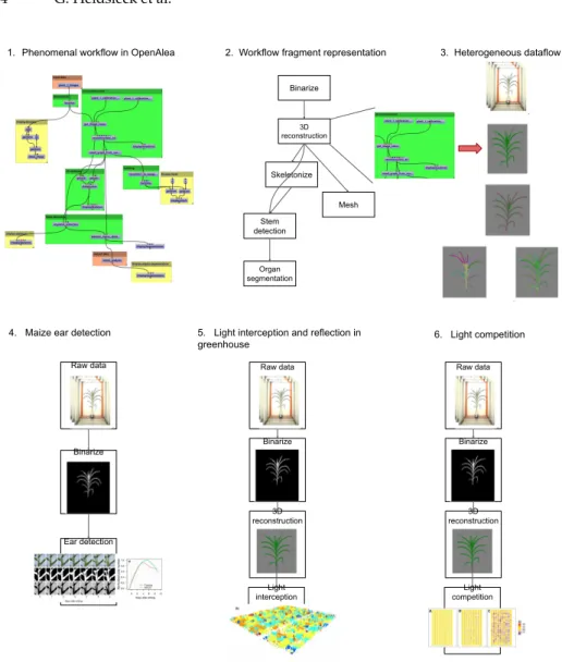
Fig. 1: Use cases in Plant Phenotyping. The different use cases are based on the OpenAlea SWfMS. 1) The Phenomenal SWf in the visual programming Ope-nAlea environment. Phenomenal SWf allows to reconstruct plants in 3D from thousands of images acquired in high-throughput phenotyping platform. The different colors represent different SWf fragments. 2) A conceptual view of the SWf with the different SWf fragments. 3) Heterogeneous raw and intermediate data such as raw RGB images, 3D plant volumes, tree skeleton, and segmented 3D mesh. 4) A SWf for maize ear detection reusing the Binarize SWf fragment. 5) A SWf reusing the Binarize and 3D reconstruction SWf fragment to compute light interception and biomass production on a reconstructed canopy. 6) The previ-ous SWf adapted to understand plant competition in variprevi-ous multi-genotype canopies.
For this purpose, we developed the OpenAlea Phenomenal software package [4]. Phenomenal provides fully automatic SWfs dedicated to 3D reconstruction, segmentation and tracking of plant organs, and light interception to estimate plant biomass in various scenarios of climatic change [28].
Phenomenal is continuously evolving with new state-of-the-art methods, thus yielding new biological insights (see Figure 1). A typical SWf is shown in Figure 1.1. It is composed of different fragments, i.e., reusable sub-workflows. In Figure 1.2, the different fragments are for binarization, 3D reconstruction, skeletonization, stem detection, organ segmentation and mesh generation:
– The Binarize fragment separates plant pixels from the background in each image. It produces a binary image from a RGB one.
– The 3D reconstruction fragment produces a 3D volume based on 12 side and 1 top binary images.
– The Skeletonisation fragment computes a skeleton inside the reconstructed volume.
– The Mesh fragment computes a 3D mesh from the volume and decimates it based on user parameters to reduce its size.
– The Stem detection fragment computes a main path in the skeleton to identify the main stem of cereal plants (e.g., maize, wheat, sorghum).
– The Organ segmentation segments the different organs on the skeleton after removal of the main stem.
Other fragments such as greenhouse or field reconstruction, or simulation of light interception, can be reused.
Based on these different SWf fragments, different users can conduct different biological analyses using the same datasets (see Figure 1.4, 1.5 and 1.6). Illus-trated in Figure 1.4, Brichet et al. ([5]) reuse the Binarize fragment to predict the flowering time in maize by detecting the apparition of the ear on maize plants. In Figure 1.5, the same Binarize fragment is reused and the 3D reconstruction fragment is added to reconstruct the volume of the 1,680 plants in 3D. This SWf reuses the same Binarize segment to reconstruct the volume of the 1600 plants in 3D (3D reconstruction fragment) and compute the light intercepted by each plant placed in a virtual scene reproducing the canopy in the glasshouse ([6, 26]). Finally, in the SWf shown in Figure 1.6, the previous SWf is reused by Chen et al. ([8]), but with different parameters to study the environmental versus the genetic influence of biomass accumulation.
These three studies have in common both the plant species (in our case maize plants) and share some SWf fragments. At least, scientists want to compare their results on previous datasets and extend the existing SWf with their own developed activities or fragments. To save both time and resources, they want to reuse the intermediate results that have already been computed rather than recompute them from scratch.
The Phenoarch platform is one of the Phenome nodes in Montpellier. It has a capacity of 1,680 plants with a controlled environment (e.g., temperature, humidity, irrigation) and automatic imaging through time. The total size of the
6 G. Heidsieck et al.
raw image dataset for one experiment is 11 Terabytes. It represents about 80000 time series of plants and about 1040000 images.
Currently, processing a full experiment with the Phenomenal SWf on local computational resources would take more than one month, while scientists require this to be done over night (12 hours). Furthermore, they need to be able to restart an analysis by modifying parameters, fix errors in the analysis or extend it by adding new processing activities. Thus, we need to use more computational resources in the cloud including both large data storage that can be shared by multiple users.
3
Cloud SWfMS Architecture
In this section, we present the proposed SWfMS architecture that integrates caching and reuse of intermediate data in the cloud. We motivate our design decisions and describe our architecture in two ways: i) in terms of functional layers (see Figure 2), which shows the different functions and components; and ii) in terms of nodes and components (see Figure 3), which are involved in the processing of SWfs.
Our architecture capitalizes on the latest advances in distributed and parallel computing to offer performance and scalability [25]. We consider a distributed architecture with on premise servers, where raw data is produced (e.g., by a phenotyping experimental platform in our use case), and a cloud site, where the SWf is executed. The cloud site (data center) is a shared-nothing cluster, i.e., a cluster of server machines, each with processor, memory and disk. We adopt shared-nothing as it is the most scalable and cost-effective architecture for big data analysis.
In the cloud, metadata management has a critical impact on the efficiency of SWf scheduling as it provides a global view of data location, e.g., at which nodes some raw data is stored, and enables task tracking during execution [20]. We organize the metadata in three repositories: catalog, provenance database and cache index. The catalog contains all information about users (access rights, etc.), raw data location and SWfs (code libraries, application code). The provenance database captures all information about SWf execution. The cache index contains information about tasks and cache data produced, as well as the location of files that store the cache data. Thus, the cache index itself is small (only file references) and the cached data can be managed using the underlying file system. A good solution for implementing these metadata repositories is a key-value store, such as Cassandra (https://cassandra.apache.org), which provides efficient key-based access, scalability and fault-tolerance through replication in a shared-nothing cluster [1].
The raw data (files) are initially produced at some servers, e.g., in our use case, at the phenotyping platform and get transferred to the cloud site. The server associated with the phenotyping platform is using iRODS [31] to grant access to the data generated. The intermediate data is placed on the node that execute the task, and is produced and processed through memory. It is only
written on disk if it is added to the cache. The cache data (files) are produced at the cloud site after SWf execution. A good solution to store these files in a cluster is a distributed file system like Lustre (http://lustre.org) which is used a lot in HPC as it scales to high numbers of files.
SWf manager (activity execution) SWf manager (activity execution)
Catalog ProvDB Cache index Catalog ProvDB Cache index
SWf data manager (files, data transfer, …) SWf data manager (files, data transfer, …)
Scheduler Cache Manager Task Manager Scheduler Cache Manager Task Manager
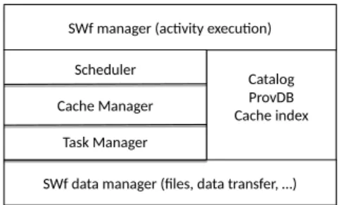
Fig. 2: SWfMS Functional Architecture
Figure 2 extends the SWfMS architecture proposed in [21], which distin-guishes various layers, to support intermediate data caching. The SWf manager is the component that the user clients interact with to develop, share and exe-cute SWfs, using the metadata (catalog, provenance database and cache index). It determines the SWf activities that need to be executed, and generates the associated tasks for the scheduler. It also uses the cache index for SWf prepro-cessing to identify the intermediate data to reuse and the tasks that need not be re-executed.
The scheduler exploits the catalog and provenance database to decide which tasks should be scheduled to cloud sites. The task manager controls task exe-cution and uses the cache manager to decide whether the task’s output data should be placed in the cache. The cache manager implements the adaptive cache provisioning algorithm described in Section 5. The SWf data manager deals with data storage, using a distributed file system.
Figure 3 shows how these components are involved in SWf processing, using the traditional master-worker model. There are three kinds of nodes, master, compute and data nodes, which are all mapped to cluster nodes at configuration time, e.g., using a cluster manager like Yarn (http://hadoop.apache.org). The master node includes the SWf manager, scheduler and cache manager, and deals with the metadata. The worker nodes are either compute or data nodes. The master node is lightly loaded as most of the work of serving clients is done by the compute and data nodes (or worker nodes), that perform task management and execution, and data management, respectively. Therefore, the master node is not a bottleneck. However, to avoid any single point of failure, there is a standby master node that can perform failover upon the master node’s failure and provide high availability.
8 G. Heidsieck et al.
Figure 3. SWfMS Technical Architecture
Cloud site Cat Cat Prov DB Prov DB Cache index Cache index Master Node (SWf mgr, schedulers) Standby Master Node Server Server Data Node (SWf data mgr) Compute Node (SWf task mgr) Data
Data (SWf data mgr)Data Node Compute Node (SWf task mgr) Data Data Raw data Raw data Server Server Raw data Raw data
Fig. 3: SWfMS Technical Architecture
Let us now illustrate briefly how SWf processing works. User clients connect to the cloud site’s master node. SWf execution is controlled by the master node, which identifies, using the SWf manager, which activities in the fragment can take advantage of cached data, thus avoiding task reexecution. The scheduler schedules the corresponding tasks that need to be processed on compute nodes which in turn rely on data nodes for data access. It also adds the transfers of raw data from remote servers that are needed for executing the SWf. For each task, the task manager decides whether the task’s output data should be placed in the cache taking into account storage costs, data size, network costs. When a task terminates, the compute node sends to its master the task’s execution information to be added in the provenance database. Then, the master node updates the provenance database and may trigger subsequent tasks.
4
Cost Model
In this section, we present our cost model. We start by introducing some terms and concepts. A SWf W(A, D) is the abstract representation of a directed acyclic graph (DAG) of computational activities A and their data dependencies D. There is a dependency between two activities if one consumes the data produced by the other. An activity is a description of a piece of work and can be a computational script (computational activity), some data (data activity) or some set-oriented algebraic operator like map or filter [22]. The parents of an activity are all activities directly connected to its inputs. A task t is the instantiation of an activity during execution with specific associated input data. The input In(t) of t is the data needed for the task to be computed, and the output Out(t) is the data produced by the execution of t. Whenever necessary, for clarity, we alternatively use the term intermediate data instead of output data. Execution data corresponds to the input and output data related to a task t. For the same activity, if two tasks tiand tjhave equal inputs, then they produce the same
output data, i.e., In(ti) = In(tj) ⇒Out(ti) = Out(tj). A SWf’s input data is the
Our approach focuses on the trade-off between execution time and cache size. In order to compare the execution time and cache size, we use a monetary cost approach, which we will also use in the experimental evaluation in Section 6. All the costs are compared at the task level and are expressed in USD. For a task t, the total cost of n executions according to the caching decision can be defined by:
Cost(t, n) = ωt∗TimeCost(t, n) + ωc∗CacheCost(t, n) (1)
where TimeCost(t, n) is the cost associated with the execution time and CacheCost (t,n) is the cost associated with caching. They represent the amount of USD spent in order to obtain the output of a task, n times. ωtand ωcrepresent the weights
of the two cost components, which are positive.
The execution time cost of a task depends on whether or not the output data of the task is added to the cache. If the output of t is not added to the cache, the execution time cost Costnocache(t, n) is the sum of the costs associated with getting
In(t) and executing t, n times. Otherwise, i.e., Out(t) is added to the cache, the execution time cost Costcache(t, n) is composed of the cost of the first execution
of t, the cost to provision the cache with Out(t) and the cost of retrieving Out(t), n-1 times. TimeCost(t, n) can be defined by:
TimeCost(t, n) = (
Costnocache(t, n), if Out(t) not in cache.
Costcache(t, n), otherwise.
(2) During workflow execution, the execution time of each task t, denoted by Timeexec(t), is stored in the provenance database. If t has already been executed,
Timeexec(t) is already known and can be retrieved from the provenance database.
When t is re-executed, its execution time is recomputed and Timeexec(t) is
up-dated as the average of all execution times. The access times to read and write in the cache are Timeread and Timewrite. Here it will be applied to input In(t) and
output Out(t) data. This time mostly dependent on the data size. Costnocache(t, n)
and Costcache(t, n) are then given by:
Costnocache(t, n) = Costcpu∗n∗[Timeread(In(t)) + Timeexec(t)] (3)
Costcache(t, n) = Costnocache(t, 1)
+Costcpu∗(n−1)∗Timeread(Out(t))
(4) where Costcpurepresents the average monetary cost to use virtual CPUs in one
determined time interval.
The cost associated with the size of the cache can be defined by:
CacheCost(t, n) = Costdisk∗size(Out(t)) (5)
where Costdiskrepresents the monetary cost of storing data in one specific time
interval, determined by the user, and size(Out(t)) is the real size of the output data generated by t execution.
10 G. Heidsieck et al.
The caching decision depends on the trade-off between the execution time cost and the storage cost. For some tasks, the output data is either much bigger in size or much complex than their input data, in this case, it is more time con-suming to retrieve data from the cache than re-executing the task (see Equation 6). This is the case for most of the tasks on plant graph generation in our SWf’s use case. In this case, no matter what is the storage cost, it is less costly to simply re-execute t. The output data generated is then not added to the cache.
Timeread(In(t)) + Timeexec(t)≤Timeread(Out(t)) (6)
In other cases, i.e., when it is time saving to retrieve the output data of a task t instead of re-executing t, the execution time cost and caching cost are compared. The output data of the task t is worth putting in the cache if for n executions of t, the cost of adding the data into the cache is smaller than the cost of an execution without cache, i.e.:
Costcache(t, n) + CacheCost(t, n)≤Costnocache(t, n) (7)
From Equations ((3)), (4), (5) and (7), we can now get the minimal number of times denoted by nmin(t), which the task t needs to be executed that it is cost
effective to add its output into the cache. nmin(t) is given by:
nmin(t) = 1 +
Timewrite(Out(t)) +
Costdisk∗size(Out(t))
Costcpu
Timeread(In(t)) + Timeexec(t)−Timeread(Out(t))
(8) We introduce p(t), the probability that t be re-executed. There is then a limit value pmin(t) that represents the minimum value of p(t) from which the output
of t is worth to add in the cache. Based on Equation (8), pmin(t) can be defined
as:
pmin(t) = nmin(t)−1 (9)
The value pmin(t) is a ratio between the cost of adding the output data of the
task t into a cache and the possible cost saved if this cached data is used instead of re-executing the task and its parents.
In the case of multiple users, the exact probability p(t) or the number of times the task t will be re-executed is not known when the SWf is executed. We then introduce a threshold ptresharbitrarily picked by the user. This threshold will be
the limit value to decide whether a task output will be added to the cache. During the execution of each task, the real values of the execution time and data size related to t are known. Thus, the caching decision is made from the Equations (6) and (9).
5
Cache Management
This section presents in detail our techniques for cache management. In our solution, cache management is involved during two main steps: SWf
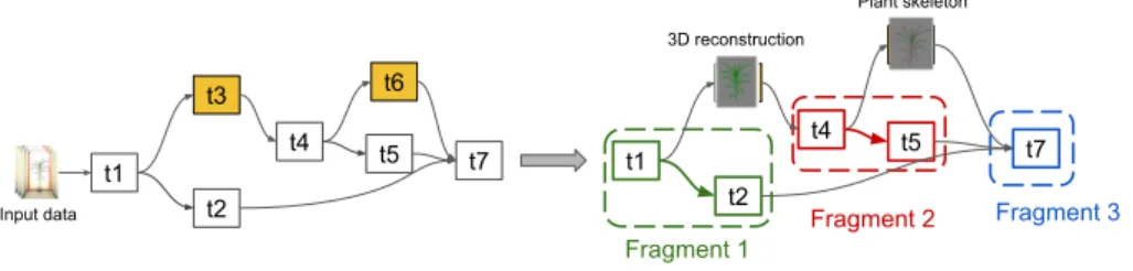
prepro-Fig. 4: DAG of tasks before preprocessing (left) and the selected fragments that need to be executed (right).
cessing and cache provisioning. The preprocessing step transforms the work-flow based on the cache by replacing workwork-flow fragments by already com-puted output data stored in the cache. The preprocessing step occurs just be-fore execution and is done by the SWf manager using the cache index. The SWf manager transform the workflow W(A, D) into an executable workflow Wex(A, D, T, Input), where T is a DAG of tasks corresponding to the activities in
A and Input is the input data. The goal of SWf preprocessing is to transform an executable workflow Wex(A, D, T, Input) into an equivalent, simpler
subwork-flow Wex′ (A′, D′, T′, Input′), where A′ is a subgraph of A with dependencies
D′, T′ is a subgraph of T corresponding to A′and Input′is a subset of Input. The preprocessing step uses a recursive algorithm that traverses the DAG T starting from the sink tasks to the source ones. The algorithm marks each task whose output is already in the cache. Then, the subgraphs of T that have each of their sink tasks marked are removed, and replaced by the associated data from the cache. The remaining graph is T′. Finally, the algorithm determines the fragments of T′: subgraphs that still need to be executed.
Figure 4 illustrates the preprocessing step on the Phenomenal SWf. The yellow tasks have their output data stored in the cache. They are replaced by the corresponding data as input for the subgraphs of tasks that need to be executed. The second step, cache provisioning, is performed during workflow execu-tion. Traditional (in memory) caching involves deciding, as data is read from disk into memory, which data to replace to make room, using a cache replacement algorithm, e.g., Least Recently Used (LRU). In our context, using a disk-based cache, the question is different. Unlike memory cache, disk-based cache makes it possible to cache the Terabytes of data generated by the SWf’s execution. Caching huge datasets has a cost and the question is to decide which task output data to place in the cache using a cache provisioning algorithm, in order to limit execution costs. This algorithm is implemented by the cache manager and used by the task manager when executing a task.
A simple cache provisioning algorithm, which we will use as baseline in the experimental evaluation, is to use a greedy method that simply stores all tasks’ output data in the cache. However, since SWf executions produce huge quantities of output data, this approach would incur high storage costs. Worse,
12 G. Heidsieck et al.
for some short duration tasks, accessing cache data from disk may take much more time than re-executing the corresponding task subgraph from the input data in memory.
Thus, we propose a cache provisioning algorithm with an adaptive method that deals with the variations in task execution times and output data complexity and sizes. The principle is to compute, for each task t, the value pmin(t) defined
in Section 4, called cache score of t, which is based on the sizes of the input and output data it consumes and produces, and the execution time of t. Depending on this value, after each task execution, the cache manager decides on whether the output data is added to the cache or not.
The cache score reveals the relevancy of caching the output data of t and takes into account the compression ratio and execution time as well as the caching costs. According to the weights provided by the user, she may prefer to give more importance to the compression ratio or executions time, depending on the storage capacity and available computational resources.
Then, during the execution of each task t, the task manager calls the cache manager to compute pmin(t). If the computed value is smaller than the threshold
ptreshprovided by the user, then t’s output data will be cached. This threshold is
arbitrarily chosen based on the probability of the SWf being re-executed.
6
Experimental Evaluation
In this section, we first present our experimental setup. Then, we present our experiments and experimental comparisons of different caching methods in terms of speedup and monetary cost in single user and multiuser scenarios. Finally, we give concluding remarks.
6.1 Experimental Setup
Our experimental setup includes the cloud infrastructure, a SWf implementation and an experimental dataset.
The cloud infrastructure is composed of one site with one data node (N1) and two identical compute nodes (N2, N3). The raw data is originally stored in an external server. During computation, raw data is transferred to N1, which contains Terabytes of persistent storage capacities. Each compute node has much computing power, with 80 vCPUs (virtual CPUs, equivalent to one core each of a 2.2GHz Intel Xeon E7-8860v3) and 3 Terabytes of RAM, but less persistent storage (20 Gigabytes).
We implemented the Phenomenal workflow (see Section 2) using OpenAlea and deployed it on the different nodes using the Conda multi-OS package manager. The master node is hosted on one of the compute nodes (N2). The metadata repositories are stored on the same node (N2) using the Cassandra key-value store. Files for raw and cached data are shared between the different nodes using the Lustre file system. File transfer between nodes is implemented with ssh.
The Phenoarch platform has a capacity of 1,680 plants with 13 images per plant per day. The size of an image is 10 Megabytes and the duration of an experiment is around 50 days. The total size of the raw image dataset represents 11 Terabytes for one experiment. The dataset is structured as 1,680 time series, composed of 50 time points (one per plant and per day).
We use a version of the Phenomenal workflow composed of 9 main activities. We execute it on a subset of the use case dataset, which is 251 of the size of the full dataset, or 440 Gigabytes of raw data, which represents the execution of 30,240 tasks.
The time interval considered for the caching time (see Section 4) is 30 days, i.e., the SWf re-executions are done within one month. The user can select longer or shorter time intervals depending on the application.
For the comparison of different cost-based caching methods, we use cost models defined in Section 4. To set the price parameters, we use prices from Amazon AWS, i.e., Costdiskis $0.1 per Gigabyte per month for storage and two
instances at $5.424 per hour for computation, i.e., Costcpuis $10.848 per hour. We
set the user’s parameters ωtand ωcat 0.5.
The caching methods we compare, defined in Section 5 are noted as:
– M1for the execution without cache.
– M2for the greedy method where all the created intermediate data produced is cached.
– M3Xfor the adaptive method, with X as the ptreshvalue. In our experiments,
X vary between 10, 40 and 160.
6.2 Experiments
We consider three experiments, based on the use case in order to analyze our caching method under different conditions:
1. This experiment aims at evaluating the scalability and speedup of the caching methods. In this experiment, we assume that the same workflow is computed three times in a month, at different times (one user at a time). This experiment is based on the SWf Phenomenal, i.e., the maize analysis (see Figure 1.4). The scalability of the SWf execution is studied using different numbers of vCPUs from 10 to 160.
2. This experiment aims at analysing the impact from the variability in execu-tion time and data size of the tasks from each activity, on the components of the proposed cost function.
3. In this experiment, the same workflow is executed with an adaptive cache strategy with different monetary costs. We assume that the same SWf is executed up to six times in a month, starting from an empty cache. This experiment shows the trade-off between better re-execution time and smaller cache size.
4. In this experiment, different users execute different SWfs that reuse sub-parts of the complete Phenomenal SWf. Depending on the caching strategy and
14 G. Heidsieck et al.
cache size, the result of some tasks may already be present in the cache. We show the impact of the value ptresh(see Section 4) on execution time, cache
size and overall monetary cost depending on the user executions.
Except for Experiment 1 where the number of vCPUs varies, it is set at 160 for the three other experiments. The execution time corresponds to the time to transfer the raw data files from the remote servers, the time to run the workflow and the time to provision the cache.
Workflow executions of the different users are serial, thus we do not consider concurrency when accessing cached data. Moreover, we assume that there are no execution or data transfer failures.
The raw data is retrieved on the data node as follows: a first file is retrieved from the remote data servers and stored in one cluster’s data node. Then, exe-cution starts using this first file while the next files are retrieved in parallel. As executing the SWf on the first file takes longer than transferring one more raw data file, we only count the time of transferring the first chunk in the execution time. 20 40 60 80 100 120 140 160 # vCPUs 2 4 6 8 speedup No cache Greedy Adaptive
(a) Speedup for one execution
20 40 60 80 100 120 140 160 # vCPUs 0 5 10 15 20 25 speedup No cache Greedy Adaptive
(b) Speedup for three executions
Fig. 5: Speedup versus number of vCPUs: without cache (orange), greedy caching (blue), and adaptive caching (green).
Speedup. In Experiment 1, we compare the speedup of the three caching meth-ods with a threshold ptresh= 40, which is optimal in this case. We define the
speedup as speedup(n) = Tn
T10, where Tnis the execution time on n vCPUs and
T10is the execution time of method M1 on 10 vCPUs.
The workflow execution is distributed on nodes N2 and N3, for different numbers of vCPUs. For one execution, Figure 5.a shows that the fastest method is M1 (orange curve). This is expected as there is no extra time spent to make data persistent and provision the cache. However, the overhead of cache provi-sioning with method M340is very small, less than 6% (green curve in Figure 5.a)
compared with method M2, up to 40% (blue curve in Figure 5.a) where all the output data are saved in the cache.
For the first execution, method M340’s overhead is only 5,6% compared to
method M1, while method M2’s overhead goes up to 40.1%. For instance, with 80 vCPUs, the execution time of method M340(i.e., 3,714 seconds) is only 5.8%
higher than execution time of method M1 (i.e., 3,510 seconds). This is much faster than method M2, which adds 2,152 seconds (1.58 times longer) of computation time in comparison with method M340. In both cases, any re-execution is much
faster than the first execution. Method M2 re-execution time is the fastest, with a speedup gain of factor that is 102 times (i.e., 34 seconds) better compared with method M1, because all the output data is already cached. Furthermore, while only the master node is working when no computation is done, the re-execution time is independent of the number of vCPUs and can be computed from a personal computer with limited vCPUs. Method M340re-execution time is 12.6
times (i.e., 258 seconds) better compared to method M1’s re-execution time. With method M340, some computation still needs to be done when the workflow is
re-executed, but such re-execution on the whole dataset can be done in a bit more than a day (i.e., 28.7 hours) on a 10 vCPUs machine, compared with 7.2 days with method M1.
For three executions starting without cache, Figure 5.b shows that method M340is much faster than the other methods (about 2.5 and 1.5 times faster of 3
executions compared to methods M1 and M2 on 80 vCPUs). Method M2 is faster than method M1 in this case, because the additional time for cache provisioning is compensated by the very short re-execution times of method M2. With 80 vCPUs, the speedup of method M340 (i.e., 18.1) is 54.70% better than that the
speedup of method M2 (i.e., 11.7) and 162.31% better than that of method M1 (i.e., 6.9). Method M340is faster than the other methods on three executions, despite
having a re-execution time higher than method M2, because the overhead of the cache provisioning is 57% smaller.
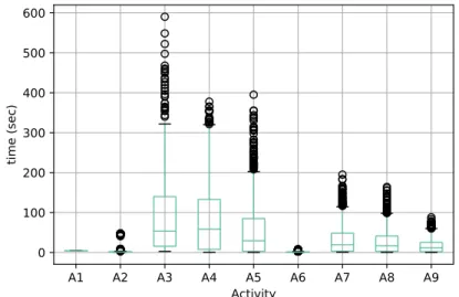
Analysis of tasks variability. The Phenomenal SWf is composed of nine activ-ities (see Section 2), which we denote by A1, A2, ..., A9. During its execution, thousands of tasks are executed that belong to the same activities. In order to assess the behavior of a task with respect to its activity, we analyze the execution time of each task per activity (see Figure 6) and the cost model through their pminvalue (see Figure 7).
In Figure 6, execution times of tasks that belong to activities A1, A2 and A6 have few variations. The tasks of such activities have predictable execution times and this information can be used to make decisions about static caching. However, the execution times of A3, A4 and A5 have high variability, which makes them unpredictable.
Figure 7 shows that the variability of the pminvalue is reduced, compared
to the variability of the execution times for activities A3 and A7. For activity A9, this is the opposite: the pminvalues for the tasks of A9 have high variability.
Note that the values of pminshown on the figure are limited at 500 for visibility
and A9 values are not entirely visible. For activities A2 and A4, the pminvalue
16 G. Heidsieck et al.
from the cache than recomputing them. This case is explained in Section 4 with Equation 6.
If the variance in the behavior of an activity’s tasks is small, then the behavior of the whole SWf execution is predictable, i.e., the tasks’ execution times and intermediate data sizes are predictable. In this case, the caching decision can be static, and done prior to execution. However, in our case, there are significant variations in the task behaviors, so we adopt an adaptive approach.
A1
A2
A3
A4
A5
A6
A7
A8
A9
Activity
0
100
200
300
400
500
600
time (sec)
Fig. 6: Execution time of each activity’s task.
Monetary cost evaluation. The first experiment shows that method M340scales
and reduces re-execution time. However, method M2 enables faster re-executions despite a longer first execution time, but it also generates more cached data. In this experiment, we evaluate the monetary costs of the various methods for the executions of SWf (see Figure 8).
The cost of method M1 comes only from the computation, as no data is stored. The whole SWf is completely re-executed so the cost increases linearly with the number of executions and ends at a total of USD 1419 for six executions. Method M2 has computation and data storage costs higher than the other two methods for the first execution. The amount of intermediate data added to the cache is huge and the total cost for the first execution is 5.96 times higher than method M1 (i.e., 1405$). However, the very small computation cost from re-execution (7.73$) compensates for the data storage cost in comparison with the method M1 after the sixth executions.
A1
A2
A3
A4
A5
A6
A7
A8
A9
Activity
0
100
200
300
400
500
p min
Fig. 7: pminof each activity’s task.
Fig. 8: Monetary cost depending on the number of users that execute the work-flow with three different cache strategies with the execution cost (blue) and the storage cost (red).
18 G. Heidsieck et al.
For the first execution, method M340adds 6% overhead in regards to method
M1’s execution cost because it populates the cache with a total of 934 Gigabytes. For any future re-executions, the decrease in computation time for method M340
makes it less expensive than method M1. For six executions, the cost gain is a factor of 3.5 (the total cost of method M340 is 409$). Method M340also has a
cost gain of a factor of 3.5 compared to M2 for six executions. The amount of intermediate data added to the cache is almost 10 times smaller for method M340
than for method M2. Thus, the data storage cost of method M2 is not worth the decrease in the computation cost compared with method M340.
This shows that method M340efficiently selects the intermediate data to be
added to the cache in order to reduce the cache size significantly while also reducing the re-execution time.
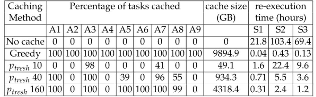
Table 1: Caching decision per task and total cache size and re-execution time for different caching methods.
Caching Percentage of tasks cached cache size re-execution
Method (GB) time (hours)
A1 A2 A3 A4 A5 A6 A7 A8 A9 S1 S2 S3 No cache 0 0 0 0 0 0 0 0 0 0 21.8 103.4 69.4 Greedy 100 100 100 100 100 100 100 100 100 9894.9 0.04 0.43 0.13 ptresh10 0 0 98 0 0 0 41 0 0 49.1 1.6 22.4 9.6 ptresh40 100 0 100 0 39 0 96 55 0 934.3 0.71 5.5 3.6 ptresh160 100 0 100 0 100 100 100 99 0 4318.4 0.31 2.4 1.2
Adding activities. In this experiment, we evaluate how the parameters of our approach impact the re-execution time, cache size and monetary cost in three different scenarios from the use case, where different SWfs are executed independently but share activities. We say that a user executes an activity from a SWf if she executes the sub-part of the SWf that leads to this activity only. The three scenarios are as follows:
1. Scenario S1 is the one presented in the monetary cost evaluation: a single user executes the last activity, i.e., A9: maize analysis, up to six times. 2. Scenario S2 involves nine users, that will each executing a different activity
of the SWf up to six times.
3. Scenario S3 involves four users: one executes activity A1, i.e., binarization, the second executes activity A3, i.e., 3D reconstruction, the third executes activity A7, i.e., maize segmentation, and the last one executes activity A9, i.e., maize analysis.
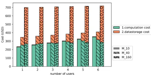
In these scenarios, each user executes a part of the SWf different from the others. Figures 9 - 11 illustrate the monetary costs for three values of ptresh: 10,
Fig. 9: Monetary cost of scenario S1: Each user executes the last activity of the SWf, for three values of ptresh.
Fig. 10: Monetary cost of scenario S2: Each user executes all the activities of the workflow, for three values of ptresh.
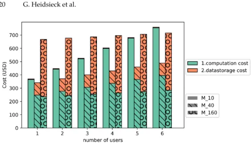
20 G. Heidsieck et al.
Fig. 11: Monetary cost of scenario S3: Each user executes the activities based on the use case (A1, A3, A7, A9), for three values of ptresh.
40 and 160. The ptreshvalues are the threshold set by the user to manage the
weight between cache size and re-execution time. With a small ptresh, only a
small portion of the output of the tasks is to be added to the cache. A larger ptresh
results in more intermediate data added to the cache.
In scenario S1, only one activity, the last one, is re-executed. As this activity is the last, without cache implies the whole SWf to be re-executed. However, as we can see in Figure 9, re-executions require little computation time even for the smallest pmin= 0.1. The re-execution times are respectively 1.6, 0.71 and 0.31
hours for methods M310, M340 and M3160(see Table 1) instead of 21.8 hours
without cache. In this scenario, the overall monetary cost of method M3160is
the highest, 49.1% higher than method M340, which we used as baseline in
the previous section. Yet, the monetary cost of method M3160remains 57.1%
smaller than that of method M2. This shows that adaptive method successfully selects the intermediate data that is the less costly to store and most worth for re-execution even in the case where a lot of intermediate data is cached.
The computation cost for the re-execution of method M310is 3.6 and 6.2 times
higher than for methods M340and M3160. However, it is the most cost-effective:
324.9$, i.e., 19.7% less than method M340’s cost. In scenario S1 where a single
activity is re-executed, a small cache size is the best option.
In scenario S2, each activity is re-executed, which represents the extreme opposite of scenario S1. In this scenario, the re-execution time for method M310
is much higher: 8.7 hours compared to 3.4 and 1.2 hours. The difference in the cache storage cost is not enough to compensate for the re-computation cost and method M310ends up being 22.8% more costly than the method M340. The
re-computation cost of method M340is also higher than in S1, and the overall
this scenario where a lot of different activities are re-executed, our method still successfully selects the right intermediate data for efficient re-execution, yet with a limited cache size.
Scenario S3 is the most representative of our use case, with different users working on specific activities, i.e., A1, A3, A7 and A9. In this scenario, the re-execution time of method M310is 4.4 times higher than that of method M340, so
the computation cost of method M310increases 4.4 times faster. Method M340is
still the cheapest one, being 8.8% and 46.4% cheaper than methods M310and
M3160. However, the computation cost is almost the same as method M3160, the
cost difference coming mostly from storage. This demonstrates that our method efficiently selects the intermediate data to cache when sub-parts of the workflow are executed separately.
6.3 Discussion
The proposed adaptive method has better speedup compared to the no cache and greedy methods, with performance gains up to 162.31% and 54.70% respectively for three executions. The execution time gain for each re-execution goes up to a factor of 60 for the adaptive method in comparison to the no cache method (i.e., 0.31 hours instead of 21.8). One requirement from the use case was to make workflow execution time shorter than half a day (12 hours). The adaptive method allows for the user to re-execute the workflow on the total dataset (i.e., 11 Terabytes) in less than one hour in the cloud and still within a day on a 10 CPUs server. In terms of monetary cost, the adaptive method yields very good gains, up to 257.8% with 6 workflow re-executions in comparison to the no cache method and 229.2% in comparison to the greedy method, which represents up to 1000$.
The experiments on several fragments of the SWf as described in the use case, show that the adaptive method succeeds in picking the most worthy intermediate data to cache. The method does work, even though the structure of the SWf is changed across executions. Similar to what happens with re-execution of a single SWf, the monetary cost of the greedy method is higher than the no cache method for up to 6 executions with different fragments or different parameters. And the execution time of greedy is always better than no cache. The adaptive method is both faster and cheaper than both no cache and greedy. The different values of the parameter ptreshallow the user to adjust between
a smaller cache size or smaller re-execution time. Table 1 shows the trade-off for three ptreshvalues. Increasing the amount of intermediate data cached obviously
decreases the re-execution time of the workflow in any scenario proposed. But the increase in cache size is not proportional to the decrease of re-execution time. The method first selects the most worthy intermediate data to add in the cache. Then, some intermediate data which is considered not beneficial, will never be added to the cache.
The method proposed in this paper focuses on finding the most cost effective intermediate data to cache during SWf execution, depending on ptreshand on the
22 G. Heidsieck et al.
in some applications and organizations, data storage may have some limitation. In this case, it could be interesting to get the optimal value of ptreshfor each
task in order to minimize the re-execution time. As the method is adaptive, the size of the total cached data is unknown until the end of the execution. However, the adaptive method could be coupled with other approaches that would approximate the final cache size. Indeed, even if tasks from the same activity have variations in their caching values and their output data sizes, an approximation could be done by taking the average value or the maximum value of some tasks for each activity, then making a static caching decision on all the rest of the tasks.
The Phenomenal workflow is data-intensive because some activities process/ generate huge datasets. Indeed, some activities are compressing the data by a significant factor, i.e., the binarization is compressing the raw data by a factor 500. Other are expending the data, i.e., the skeletonization is expanding the data by a factor 100 (it generates 2TB of data while consuming only 30GB). The Phenomenal workflow is also compute-intensive, as some activities require long computing time, i.e., the 3D reconstruction require 1200 hours of total computing time. The Phenomenal workflow is representative of many other data science workflows, that perform long analyses on huge datasets. Thus, the method presented would work on data-intensive workflows where the execution time is significant with regards to the data transfers times However, the method is not suitable for any kind of application. It adds an overhead when the workflow is executed, thus it would be inefficient on workflows that are not data- or compute-intensive.
7
Related Work
Storing and reusing intermediate data in SWf executions can be found in several SWfMSs [7, 30]. However, there is no definitive solution for two important prob-lems: 1) how to automatically reuse SWf fragments in multiple SWf’s executions. 2) what intermediate data to cache if there is not provenance data available. The related works either focus on an optimized solution for selecting a specific portion of data to cache when all provenance and reuse information are known, or automatic caching for the same SWf.
Different SWfMSs, such as Kepler, VisTrails, OpenAlea, exploit intermediate data for SWf re-execution. Each of these systems has its unique way of addressing data reuse. OpenAlea [30] uses a cache that captures the intermediate results in main memory. When a SWf is executed, it first accesses the cached data. However, the OpenAlea cache is local and main memory-based, while the approach proposed in this paper is distributed and persistent. VisTrails provides visual analysis of SWf results and captures the evolution of SWf provenance, i.e., the steps of the workflow at each execution, as well as the intermediate data from each execution [7]. The intermediate data are then reused when previous tasks are re-executed. This approach allows the user to change parameters or activities in the workflow and efficiently re-execute each workflow activity to
analyze the different results. This solution for caching intermediate data has been extended to generate ßtrong links"between provenance and execution [19] [12]. The intermediate data cache is associated with provenance to enhance reproducibility, and the intermediate data that has been cached is always reused. However, VisTrails does not take distribution into account when storing and using the cache, and the selection of the data to be stored becomes manual as the size of the intermediate data increases. Our approach is different as it works in a distributed environment where data transfer costs may be significant.
Storing intermediate data in the cloud may be also beneficial. However, the trade-off between the cost of re-executing tasks and the costs of storing intermediate data is not easy to estimate [2, 11]. Yuan et al. [34] propose an algorithm based on the ratio between re-computation cost and storage cost at the task level. The algorithm is based on a graph of dependencies between the intermediate data sets, generated from the provenance data. Then, the cost of storing each intermediate data set is weighted by the number of dependencies in the graph. The algorithm computes the optimized set of intermediate data sets that need to have minimum cost. The algorithm is improved in [35] to take into account workflow fragments. Both algorithms are used before the workflow execution, using the provenance data of the intermediate datasets. They provide near optimal caching intermediate datasets selection. However, this approach requires global knowledge of executions, such as the execution time of each task, the size of each data set and the number of incoming re-executions. This optimization is also based on a single workflow and is not adapted to changing workflows. Our approach is different as it provides efficient caching of intermediate data in evolving workflows.
Kepler [3] provides intermediate data caching for single-site cloud SWf execution. It uses a remote relational database where intermediate data is stored after workflow execution. Two steps are added when executing a workflow. First, the cache database is checked and all intermediate cached data is sent to a specific cloud site before execution. To reduce storage cost, the intermediate data that need to be cached are determined based on how many times the workflow will be re-executed in a given period of time [9]. Finally, reuse is done at the entire workflow level, whereas our solution is finer grain, working at the activity level.
Other approaches propose solutions for caching data in MapReduce work-flows. Zhang et al. [37] use the Memcached distributed memory caching system to cache the intermediate data between Map and Reduce operations. This approach focuses on a single MapReduce job, and the cached data is not persistent and reused across executions. Elghandour et al. [13] propose a system to manage and cache intermediate data of MapReduce jobs for future reuse. Olston et al. [24] propose two caching strategies on top of the Pig language and propose different methods to manage persistent intermediate data. The problem of this approach is that it is static, i.e., they do not consider automatic caching. Gottin et al. [15] propose an algorithm that finds an optimized cache decision plan for a dataflow execution in Apache Spark. The approach is based on a cost model that
24 G. Heidsieck et al.
uses provenance data, and tries the possible combinations of caching selection in order to select the best one. This approach does not scale with the size of the SWf, and the caching decision still falls in the hands of the user.
8
Conclusion
In this paper, we proposed an adaptive caching solution for efficient execution of data-intensive workflows in the cloud. Our solution automatically manages the storage and reuse of intermediate data, and is adaptive in terms of variations in task execution times and output data size. The adaptive aspect of our solution is to take into account task compression behavior.
We implemented our solution in the OpenAlea SWfMS and performed exten-sive experiments on real data with the Phenomenal SWf, a real big workflow that consumes and produces around 11 TB of raw data. We compared three methods : no cache, greedy, and adaptive. Our experimental evaluation shows that the adaptive method allows for caching only the relevant output data for subsequent re-executions by other users, without incurring a high storage cost for the cache. The results show that adaptive caching can yield major performance gains, e.g., up to a factor of 3.5 with 6 workflow re-executions.
In this paper, we focused on reducing the monetary cost of running multiple workflows by caching and reusing intermediate data. While our technique show an improvement with respect to greedy approaches, we notice that the scaling up is limited (see Figure 5). In the case of multiple users, the cloud computing and storage capacities might be a bottleneck to scale up workflow executions. In the use case, multiple cloud sites are available. A next step would be to extend our method to multisite clouds.
The architecture proposed is based on disk storage for data reuse. Writing and reading the cached data on disk adds an significant overhead. A next step to improve our cache architecture would be to add an in memory cache for some of the most used cached data.
This work represents a step forward in experimental science like biology, where scientists extend existing workflows with new methods or new parame-ters to test their hypotheses on datasets that have been previously analyzed.
Acknowledgments. This work was supported by the #DigitAg French Conver-gence Lab. on Digital Agriculture (http://www.hdigitag.fr/com), the SciDISC Inria associated team with Brazil, the Phenome-Emphasis project (ANR-11-INBS-0012) and IFB (ANR-11-INBS-0013) from the Agence Nationale de la Recherche and the France Grille Scientific Interest Group.
References
1. Abramova, V., Bernardino, J., Furtado, P.: Testing cloud benchmark scalability with cassandra. In: 2014 IEEE World Congress on Services. pp. 434–441. IEEE (2014)
2. Adams, I.F., Long, D.D., Miller, E.L., Pasupathy, S., Storer, M.W.: Maximizing efficiency by trading storage for computation. In: HotCloud (2009)
3. Altintas, I., Barney, O., Jaeger-Frank, E.: Provenance collection support in the kepler scientific workflow system. In: International Provenance and Annotation Workshop. pp. 118–132 (2006)
4. Artzet, S., Brichet, N., Chopard, J., Mielewczik, M., Fournier, C., Pradal, C.: Ope-nalea.phenomenal: A workflow for plant phenotyping (Sep 2018)
5. Brichet, N., Fournier, C., Turc, O., Strauss, O., Artzet, S., Pradal, C., Welcker, C., Tardieu, F., Cabrera-Bosquet, L.: A robot-assisted imaging pipeline for tracking the growths of maize ear and silks in a high-throughput phenotyping platform. Plant Methods 13(1), 96 (2017)
6. Cabrera-Bosquet, L., Fournier, C., Brichet, N., Welcker, C., Suard, B., Tardieu, F.: High-throughput estimation of incident light, light interception and radiation-use efficiency of thousands of plants in a phenotyping platform. New Phytologist 212(1), 269–281 (2016)
7. Callahan, S.P., Freire, J., Santos, E., Scheidegger, C.E., Silva, C.T., Vo, H.T.: Vistrails: visualization meets data management. In: ACM SIGMOD Int. Conf. on Management of Data (SIGMOD). pp. 745–747 (2006)
8. Chen, T.W., Cabrera-Bosquet, L., Alvarez Prado, S., Perez, R., Artzet, S., Pradal, C., Coupe-Ledru, A., Fournier, C., Tardieu, F.: Genetic and environmental dissection of biomass accumulation in multi-genotype maize canopies. Journal of Experimental Botany (2018)
9. Chen, W., Altintas, I., Wang, J., Li, J.: Enhancing smart re-run of kepler scientific workflows based on near optimum provenance caching in cloud. In: IEEE World Congress on Services (SERVICES). pp. 378–384 (2014)
10. Cohen-Boulakia, S., Belhajjame, K., Collin, O., Chopard, J., Froidevaux, C., Gaignard, A., Hinsen, K., Larmande, P., Le Bras, Y., Lemoine, F., et al.: Scientific workflows for computational reproducibility in the life sciences: Status, challenges and opportunities. Future Generation Computer Systems (FGCS) 75, 284–298 (2017)
11. Deelman, E., Singh, G., Livny, M., Berriman, B., Good, J.: The cost of doing science on the cloud: the montage example. In: International Conference forHigh Performance Computing, Networking, Storage and Analysis. pp. 1–12 (2008)
12. Dey, S.C., Belhajjame, K., Koop, D., Song, T., Missier, P., Ludäscher, B.: Up & down: Improving provenance precision by combining workflow-and trace-level information. In: USENIX Workshop on the Theory and Practice of Provenance (TAPP) (2014) 13. Elghandour, I., Aboulnaga, A.: Restore: reusing results of mapreduce jobs. Proceedings
of the VLDB Endowment 5(6), 586–597 (2012)
14. Garijo, D., Alper, P., Belhajjame, K., Corcho, O., Gil, Y., Goble, C.: Common motifs in scientific workflows: An empirical analysis. Future Generation Computer Systems (FGCS) 36, 338–351 (2014)
15. Gottin, V.M., Pacheco, E., Dias, J., Ciarlini, A.E., Costa, B., Vieira, W., Souto, Y.M., Pires, P., Porto, F., Rittmeyer, J.G.: Automatic caching decision for scientific dataflow execution in apache spark. In: Proceedings of the 5th ACM SIGMOD Workshop on Algorithms and Systems for MapReduce and Beyond. p. 2. ACM (2018)
16. Heidsieck, G., Oliveira, D., Pacitti, E., Pradal, C., Tardieu, F., Valduriez, P.: Adaptive caching for data-intensive scientific workflows in the cloud. In: Int. Conf. on Databases and Expert Systems Applications (DEXA). pp. 1–15 (2019), to Appear
17. Juve, G., Deelman, E.: Scientific workflows in the cloud. In: Grids, clouds and virtualization, pp. 71–91. Springer (2011)
26 G. Heidsieck et al.
18. Kelling, S., Hochachka, W.M., Fink, D., Riedewald, M., Caruana, R., Ballard, G., Hooker, G.: Data-intensive science: a new paradigm for biodiversity studies. BioScience 59(7), 613–620 (2009)
19. Koop, D., Santos, E., Bauer, B., Troyer, M., Freire, J., Silva, C.T.: Bridging workflow and data provenance using strong links. In: Int. Conf. on Scientific and Statistical Database Management (SSDBM). pp. 397–415 (2010)
20. Liu, J., Morales, L.P., Pacitti, E., Costan, A., Valduriez, P., Antoniu, G., Mattoso, M.: Efficient scheduling of scientific workflows using hot metadata in a multisite cloud. IEEE Trans. on Knowledge and Data Engineering pp. 1–20 (2018)
21. Liu, J., Pacitti, E., Valduriez, P., Mattoso, M.: A survey of data-intensive scientific workflow management. Journal of Grid Computing 13(4), 457–493 (2015)
22. Ogasawara, E., Dias, J., Oliveira, D., Porto, F., Valduriez, P., Mattoso, M.: An algebraic approach for data-centric scientific workflows. Proc. of the VLDB Endowment (PVLDB) 4(12), 1328–1339 (2011)
23. de Oliveira, D., Baião, F.A., Mattoso, M.: Towards a taxonomy for cloud computing from an e-science perspective. In: Cloud Computing. Computer Communications and Networks., pp. 47–62. Springer (2010)
24. Olston, C., Reed, B., Silberstein, A., Srivastava, U.: Automatic optimization of parallel dataflow programs. In: USENIX Annual Technical Conference. pp. 267–273 (2008) 25. Özsu, M.T., Valduriez, P.: Principles of Distributed Database Systems, Third Edition.
Springer (2011)
26. Perez, R.P., Fournier, C., Cabrera-Bosquet, L., Artzet, S., Pradal, C., Brichet, N., Chen, T.W., Chapuis, R., Welcker, C., Tardieu, F.: Changes in the vertical distribution of leaf area enhanced light interception efficiency in maize over generations of maize selection. Plant, cell & environment (2019)
27. Pradal, C., Artzet, S., Chopard, J., Dupuis, D., Fournier, C., Mielewczik, M., Negre, V., Neveu, P., Parigot, D., Valduriez, P., et al.: Infraphenogrid: a scientific workflow infrastructure for plant phenomics on the grid. Future Generation Computer Systems (FGCS) 67, 341–353 (2017)
28. Pradal, C., Cohen-Boulakia, S., Heidsieck, G., Pacitti, E., Tardieu, F., Valduriez, P.: Distributed management of scientific workflows for high-throughput plant phenotyping. ERCIM News 113, 36–37 (2018)
29. Pradal, C., Dufour-Kowalski, S., Boudon, F., Fournier, C., Godin, C.: Openalea: a visual programming and component-based software platform for plant modelling. Functional plant biology 35(10), 751–760 (2008)
30. Pradal, C., Fournier, C., Valduriez, P., Cohen-Boulakia, S.: Openalea: scientific workflows combining data analysis and simulation. In: Int. Conf. on Scientific and Statistical Database Management (SSDBM). p. 11 (2015)
31. Rajasekar, A., Moore, R., Hou, C.y., Lee, C.A., Marciano, R., de Torcy, A., Wan, M., Schroeder, W., Chen, S.Y., Gilbert, L., et al.: irods primer: integrated rule-oriented data system. Synthesis Lectures on Information Concepts, Retrieval, and Services 2(1), 1–143 (2010)
32. Roitsch, T., Cabrera-Bosquet, L., Fournier, A., Ghamkhar, K., Jiménez-Berni, J., Pinto, F., Ober, E.S.: Review: New sensors and data-driven approaches—a path to next generation phenomics. Plant Science (2019)
33. Tardieu, F., Cabrera-Bosquet, L., Pridmore, T., Bennett, M.: Plant phenomics, from sensors to knowledge. Current Biology 27(15), R770–R783 (2017)
34. Yuan, D., Yang, Y., Liu, X., Chen, J.: A cost-effective strategy for intermediate data storage in scientific cloud workflow systems. In: IEEE Int. Symp. on Parallel & Distributed Processing (IPDPS). pp. 1–12 (2010)
35. Yuan, D., Yang, Y., Liu, X., Li, W., Cui, L., Xu, M., Chen, J.: A highly practical approach toward achieving minimum data sets storage cost in the cloud. IEEE Trans. on Parallel and Distributed Systems 24(6), 1234–1244 (2013)
36. Zhang, J., Votava, P., Lee, T.J., Chu, O., Li, C., Liu, D., Liu, K., Xin, N., Nemani, R.: Bridging vistrails scientific workflow management system to high performance computing. In: 2013 IEEE Ninth World Congress on Services. pp. 29–36. IEEE (2013) 37. Zhang, S., Han, J., Liu, Z., Wang, K., Feng, S.: Accelerating mapreduce with distributed memory cache. In: 2009 15th International Conference on Parallel and Distributed Systems. pp. 472–478. IEEE (2009)