Differentiated green loans

HAL Id: hal-01890636

https://hal.archives-ouvertes.fr/hal-01890636v2

HAL is a multi-disciplinary open access archive for the deposit and dissemination of sci-entific research documents, whether they are pub-lished or not. The documents may come from teaching and research institutions in France or abroad, or from public or private research centers.

L’archive ouverte pluridisciplinaire HAL, est destinée au dépôt et à la diffusion de documents scientifiques de niveau recherche, publiés ou non, émanant des établissements d’enseignement et de recherche français ou étrangers, des laboratoires publics ou privés.

Differentiated green loans

Louis-Gaëtan Giraudet, Anna Petronevich, Laurent Faucheux

To cite this version:

Louis-Gaëtan Giraudet, Anna Petronevich, Laurent Faucheux. Differentiated green loans. Energy Policy, Elsevier, 2021, 149, pp.111861. �10.1016/j.enpol.2020.111861�. �hal-01890636v2�

1

Differentiated green loans

Louis-Gaëtan Giraudet, Anna Petronevich, Laurent Faucheux

Preprint for Energy Policy*

Scaling up home energy retrofits requires that associated loans be priced efficiently. Using a unique dataset of posted loan prices scraped from online simulators made available by French credit institutions, we examine the differentiation of interest rates in relation to project risk. Crucially, our data are immune from sorting bias based on borrower characteristics. We find that greener, arguably less risky, automobile projects carry lower interest rates, but greener home retrofits do not. On the other hand, conventional automobiles carry lower interest rates than do conventional home retrofits, despite arguably similar risk. Our results are robust to a range of robustness checks, including placebo tests. They together suggest that lenders use underlying assets to screen borrower’s unobserved willingness to pay, which can cause under-investment in home energy retrofits. We thereby point to a new form of the energy efficiency gap. This has important policy implications in that it can explain low uptake of zero-interest green loan programs.

JEL: D14, G21, Q41

Keywords: personal loan, home energy retrofit, screening, data scraping, online prices, energy efficiency gap

Correspondence. giraudet@centre-cired.fr and anna.petronevich@banque-france.fr. Affiliations. Giraudet: Ecole des Ponts ParisTech, CIRED. Petronevich: Banque de France. Faucheux: CNRS, CIRED. CRediT author statement. Giraudet: Conceptualization, funding acquisition, supervision, writing. Petronevich: data curation, formal analysis, writing. Faucheux: software, investigation, data curation. Acknowledgments. We gratefully acknowledge funding from the European Investment Bank Institute under the University Research Sponsorship Programme, Grant EIBI/KnP/TT/ck (1-RGI-C311). We thank Dominique Berthon for excellent research assistance that set the stage for the project. We thank Jean Barthélémy, Patricia Crifo, Leonardo Gambacorta, Mattia Girotti, Sven Heim, Sébastien Houde, Christian Huse, Elisabetta Iossa, Claire Labonne, Antoine Lallour, Maria Loumioti, Antoine Mandel, Tien Viet Nguyen, Julia Schmidt and seminar participants at ETH Zürich and CERNA Mines ParisTech for useful comments on earlier drafts. The views expressed in this paper do not necessarily reflect the opinion of the Banque de France. All remaining errors are ours.

* Submitted 2 March 2020; Received in revised form 19 June 2020; Accepted 14 August 2020; Corrected proofs submitted 3 September 2020.

2

1 Introduction

Credit markets are characterized by information asymmetries about borrower risk, conducive to rationing. The problem, first pointed out in the late 1970s (Jaffe and Russell, 1976; Stiglitz and Weiss, 1981), has since largely been mitigated thanks to the advent of information technologies. Reduction in computation and data storage costs allowed credit institutions to routinely compute credit scores and use them to screen unobservable borrower risk. This gave rise to price differentiation – less risky borrowers being charged lower interest rates – resulting in an expansion of various forms of consumer credit, including mortgages, unsecured personal loans and credit card debt (Edelberg, 2006; Athreya et al., 2012; Einav et al., 2013; Sánchez, 2018). In addition, an increasing sophistication of loan contracts allowed firms to use other screening devices, such as dynamic repayment incentive (Karlan and Zinman, 2009) or down payments (Einav et al., 2012), to mitigate the residual risk.

While evidence is growing about how lenders value borrower characteristics, little is known about how they value the risk associated with the assets consumers borrow for, and how the two dimensions interact in loan pricing. Evidence is provided by Bičáková (2007) that default rates vary across projects due to adverse selection – borrowers with different creditworthiness tend to purchase different types of goods on credit – and, to a lesser extent, moral hazard – purchasing certain goods on credit affects the likelihood of default. Though this is the only empirical study we are aware of that examines the role asset types play in consumer credit,1 her dataset does not allow the author to examine how interest rates are affected by the identified information asymmetries.

The problem is particularly important when it comes to energy-using assets, which play a major role in anthropogenic global warming. The operation of energy-using assets in the building and transportation sectors contributes 30% of global emissions, two thirds of which can be attributed to households. Improving their energy efficiency is recognized as the most cost-effective means of reducing carbon dioxide emissions. Limiting global warming to 2°C above pre-industrial levels would thus require global investment in energy efficiency ranging from $700 billion to $1.3 trillion per year in 2050 (IPCC, 2018; IEA, 2018). With upfront costs typically in the thousands of dollars, many energy-efficient assets are purchased on credit. Scaling up energy efficiency therefore requires that sizable borrowing needs be satisfied in an economically efficient manner. Although some credit constraints have been pointed out as hindering energy efficiency investment (Berry, 1984; Palmer et al., 2012), they have yet to be characterized. In particular, it remains to determine whether they are simple market barriers – after all, investment decisions are all about maximizing return under credit constraints – or whether there is something more specific to them in the context of energy efficiency (e.g., information asymmetries) that makes them a market failure.

Our goal in this paper is to fill these research gaps and document how interest rates vary with the characteristics of the asset underlying the loan, with particular attention to their energy efficiency. Specifically, we consider a range of energy-using assets that are important in the market for personal loans, namely renovations and automobiles, and investigate how their energy efficiency affects the price

1 _{There also exists theoretical research on the issue that looks at how information asymmetries about product}

3 of the associated loan. Energy efficiency investments are an ideal candidate for conducting such an analysis in that they provide a simple testable prediction: By reducing energy operating costs, they increase the borrower’s ability to repay and the resale value of his or her asset, both of which lower project risk (e.g., Brounen and Kok, 2011; for a review, see Giraudet, 2020). A well-functioning credit market should therefore offer lower interest rates for energy efficient projects (hereafter “green projects”) than for projects devoid of that attribute but otherwise similar (hereafter “conventional projects”).

Despite the importance of the issue, the way home energy efficiency is valued in credit markets has received surprisingly little attention. A few studies examine the relationship between home energy efficiency and default rates on mortgages. Kaza et al. (2014) and An and Pivo (2018) both find that greener buildings entail lower default rates, respectively in the US residential and commercial sector. This finding, corroborated in ongoing studies by Billio et al. (2020) on the Netherlands and Guin and Korhonen (2020) on the United Kingdom, confirms that green projects are less risky than are conventional projects, which is the form of moral hazard discussed by Bičáková (2007).2 In contrast, the relationship between loan terms and home energy efficiency is, to our knowledge, only studied by An and Pivo (2018). Using ex post data from a commercial mortgage program, the authors find that those buildings that were certified green at loan origination obtained slightly but statistically significantly better loan terms than did their conventional counterparts. This result tends to support the simple prediction that greener investments should carry lower interest rates. Its internal validity is however threatened by selection issues, as the authors could not control for borrowers’ characteristics.

To overcome the data limitations faced in previous studies looking at the role of assets – green ones in particular – in consumer credit, we assembled a unique panel dataset of loan terms posted on credit institutions’ websites. The data were retrieved every week, in 2015 and 2016, from loan simulators made available online by 15 institutions which cover the near totality of the French market. Our approach differs from those of Bičáková (2007) and An and Pivo (2018) in several respects. First and foremost, our data are immune from sorting bias in relation to borrower characteristics (e.g., income, credit score) and contract terms (e.g., collateral), as the online simulators they originate from only query information about the loan size, duration and purpose. We therefore avoid the selection issues faced by An and Pivo (2018). Second, our scope combines the breadth of Bičáková (2007), who covers different types of household investments (automobile, equipment, etc.) and the depth of An and Pivo (2018), who focus on green vs. non-green buildings.3 Such an extensive focus allows us to examine how the green aspect interacts with the designation of the project. Third, these facilitating features come at the cost of handling ex ante, rather than ex post, data. This implies in particular that we cannot study default rates.

2

Note that this finding does not seem to carry over to energy-efficient transportation, as evaluations of the Efficient-location mortgage program suggest (Blackman and Krupnick, 2001; Kaza et al., 2016).

3 _{In addition, An and Pivo (2018) study mortgage loans for new commercial buildings, while we study unsecured}

loans for household investment. When it comes to buildings, we are concerned with the renovation of existing ones rather than new constructions. Given the slow turnover of building stocks (typically 1% every year), the renovation of existing buildings is much more crucial for carbon dioxide emission reductions than are new constructions. This is especially true in the residential building stock, which is typically 50% larger than the commercial building stock.

4 Notwithstanding, the dynamics of our posted rates closely follows that of realized rates on personal loans, which lends external validity to our analysis.

We investigate two hypotheses – whether green projects are offered lower interest rates than their conventional counterparts on the one hand, and whether renovation and vehicle projects are priced the same, regardless of any green attribute, on the other. We do so by estimating a parsimonious econometric model of interest rate margin that includes time and institution fixed effects and controls for loan characteristics. When considering the period as a whole, we fail to reject the first hypothesis; we additionally find higher interest rates for renovations than for retrofits, which leads us to reject the second hypothesis. Overall effects are small (except for green vehicles) but statistically significant and confirmed by statistical tests and robustness checks, including placebo tests. Looking at each year separately, we find that both results hold for 2016 but were inverted in 2015. In other words, the market seems to increasingly value the lower risk associated with green projects while increasingly offering higher interest rates for renovation projects than for vehicles. The effect is particularly pronounced for short-term loans (12 months) and, somewhat surprisingly, for banking groups that own a green certification (TEEC, ISR or PRI). Lastly, when fixed effects are replaced by macroeconomic and financial factors, only unemployment appears to have a significant – actually negative – effect on interest rates.

Our results contribute to two strands of the literature – the economics of energy efficiency and household finance. Regarding the former, by documenting relatively high interest rates for home energy retrofits, we highlight new factors conducive to under-investment in energy-efficient technologies – a phenomenon known as the energy-efficiency gap (Jaffe and Stavins, 1994). While most research into the issue has focused on behavioral factors on the demand side (Gillingham et al., 2009; Allcott and Greenstone, 2012; Gerarden et al., 2017), we focus on less-studied supply-side factors. Specifically, we add to the scarce literature on energy efficiency loans (Berry, 1984; Palmer et al., 2012; Kaza et al., 2014; An and Pivo, 2018) by emphasizing the interaction between the green attribute and other dimensions of the underlying asset. In particular, we find that lenders may internalize information asymmetries between homeowners and retrofit contractors that have been found to mitigate energy savings (Giraudet et al., 2018b). Our analysis leads us to the conclusion that the credit constraints often pointed out in the context of energy efficiency are more likely to be market failures than simple market barriers. This has important implications for the evaluation of loan policies for energy efficiency investments, such as Property Assessed Clean Energy (PACE) Financing in the United States and the zero-interest loan program (Eco-prêt à taux zero) in France.4 Though research into these programs is still in its infancy, preliminary evidence exists that the latter is strongly underperforming (Giraudet et al., 2018a). Our results can provide an explanation for this ineffectiveness: If, as we show, lenders are able to charge high interest rates for home energy retrofits in laissez-faire, the Government needs to offer them generous

4

Another program worth mentioning is the Green Deal in the United Kingdom, which was phased out soon after roll-out (Rosenow and Eyre, 2016). In addition to such programs targeting personal loans for energy efficiency improvements, other programs target mortgages backed by energy-efficient property. Those include the Energy Efficiency Mortgage Action Plan (EeMAP) of the European Commission and the LENDERS Project in the United Kingdom. In France, there are important differences between the mortgage and personal loan markets: the amounts borrowed typically differ by one order of magnitude; mortgage interest rates are also significantly lower. The extent to which our results extend to the mortgage market should therefore be assessed with caution.

5 subsidies in order to make them willing to issue zero-interest loans. This is only feasible within the boundaries of the Government’s budget. The important transfers it implies from taxpayers to credit institutions moreover raises distributional concerns. In a broader perspective, we also contribute to the emerging literature on green finance. We complement existing studies showing that financial markets increasingly value portfolios including green assets (Eichholtz et al., 2012), green bounds (Karpf and Mandel, 2018; Zerbib, 2019) and environmental ratings (Capelle-Blancard et al., 2019) by highlighting how these effects are transmitted to the loan retail market.

Our second contribution more generally relates to household finance, a field that is known for crucially lacking stylized facts (Campbell, 2006; Zinman, 2014). We document an anomaly, namely systematic differences between the interest rates offered for renovation- and for vehicle-backed loans. While the risks associated with these projects should not particularly differ for a given borrower, we observe a small but persistent difference of about 0.15 percentage points, or 5% of the loan price. Following Bičáková (2007), this could be explained by two effects. One is moral hazard: the fact that an automobile can more easily be sold on a second-hand market than a home renovation (which cannot be separated from the home itself) creates stronger incentives to repay the loan in the former case. Another possible explanation is adverse selection: the two types of goods may be correlated with different repayment behaviors. In this regard, the most plausible conjecture we think a lender would make is that those consumers that purchase a home renovation are more likely to be a homeowner, hence be wealthier, than those purchasing an automobile. If this is the case, however, the differentiation we observe goes in the opposite direction from that uncovered by Bičáková (2007): we indeed find that loans presumably taken by wealthier borrowers carry higher interest rates. One way to reconcile our findings with adverse selection is to consider that lenders’ screening strategy is motivated by surplus extraction (assuming that wealthier borrowers have a higher willingness to pay), rather than by risk management (assuming that wealthier borrowers present a lower risk profile). Our additional finding that unemployment has a significant, negative effect on interest rates lends support to this hypothesis. This hypothesis may have important welfare implications since, unlike risk-based screening, screening motivated by surplus extraction might generate credit rationing at the low end of the risk distribution. More research is therefore needed to assess the validity of the ‘surplus extraction’ hypothesis. Anyway, the competing effects discussed here illustrate the ‘uniqueness of credit’ (Melzer and Morgan, 2015) in that it shares the characteristics of a conventional good and of a financial product.

The analysis proceeds as follows. Section 2 formulates testable hypotheses. Section 3 describes the data. Section 4 details the empirical approach. Section 5 provides estimation results. Section 6 provides robustness checks. Section 7 discusses welfare implications and concludes.

2 Testable hypotheses

Here we formulate hypotheses that our dataset allows us to test. As discussed in the introduction, basic principles of finance imply the following:

6 Rejection of this hypothesis can be interpreted as evidence of an energy efficiency gap. An increasing number of studies point to energy retrofit projects that fail to deliver predicted energy savings (Metcalf and Hassett, 1999; Graff Zivin and Novan, 2016; Fowlie et al., 2018). While these studies attribute the missing savings to modeling flaws in engineering calculations, Giraudet et al. (2018b) propose an alternative explanation rooted in information asymmetries. Evaluating a home weatherization program conducted in Florida, the authors provide evidence that retrofit contractors engage in moral hazard by under-providing quality in hard-to-observe measures such as insulation installation or duct sealing. Lenders might anticipate these problems and price energy-efficient assets the same as conventional, non-energy-efficient assets. Hypothesis 1 could also be rejected if green projects are subsidized and lenders take advantage of some market power to extract the borrower’s surplus from the subsidy. If this is to happen, considering that existing subsidies are of the same order of magnitude for automobiles and retrofits in France (see Appendix A), we expect the green effect to go in this same direction for both types of asset.

Now, regardless of any energy efficiency consideration, a renovation and a vehicle are two household investments which, as a first approximation, carry comparable risk. In a well-functioning credit market, the following hypothesis should therefore hold:

Hypothesis 2: The interest rates for renovation and vehicle projects are identical.

As discussed in the introduction, this hypothesis may however be rejected under the following circumstances: moral hazard, assuming that unlike automobiles, retrofits cannot be resold on second-hand markets, which strengthens incentive to default in that case; lenders using the loan designation as a screening device of unobserved borrowing characteristics, with two possible motivations – risk management or surplus extraction. While moral hazard and adverse selection motivated by surplus extraction lead to higher interest rates for renovations than for vehicles, adverse selection motivated by risk management leads to the opposite. This leads us to consider an amended version of Hypothesis 2:

Hypothesis 2’: Vehicle projects carry lower interest rates than do renovation projects.

Hypothesis 2’ can be interpreted as dominance of the first two mechanisms over the third. Unlike risk management, surplus extraction may reduce welfare by driving some borrowers out of the market.

3 Data

3.1 The French market for personal loans

We start with providing some background about the importance of the French market for personal loans. Appendix A provides additional background on environmental policies that are important to consider when examining how lenders set interest rates.

France ranks third in Europe in terms of total consumer credit outstanding – behind the United Kingdom and Germany – and second in terms of outstanding per capita – behind the United Kingdom. In 2016,

7 7.36 million (26%) of households held a form of consumer credit,5 with a total outstanding of €160 billion. The average loan has a size of 11,449€ and a duration of 47 months. Personal loans, which are our product of interest, were the main form of consumer credit, covering 45% of the outstanding. Loans tied to a specific purchase (crédit affecté, typically supplied by product retailers in partnership with a credit institution), covered 9% of the outstanding; though not the focus of our analysis, these are important to consider, as they can be used for the same type of purchase as personal loans (Meilleurtaux.com, 2015; ACPR, 2016; Mouillard, 2017; Eurogroup, 2018).

Consumer credit was dedicated to financing the following purchases: 47% to vehicles; 19% to equipment purchase, including appliances; 10% to home retrofits; 8% to consumption; 8% to liquidity; 4% to credit restructuring; and 4% to tax payments (Mouillard, 2017). While automobiles and home investments form the bulk of credit purposes, the associated loans take different forms. On the automobile segment, 75% of purchases involve credit, which is shared between personal loans, loans tied to purchase, and leasing contracts (SOFINCO, 2010). On the home segment, 32% of retrofits involve credit – mostly personal loans – covering over 50% of the upfront cost (Ademe, 2018).6 The borrower profiles also differ between automobile and home investment loans, with borrowers on average seven years older in the latter case (Meilleurtaux.com, 2015). In addition, it is worth noting that home energy retrofits are essentially conducted by homeowners (79% in France, according to Ademe, 2018), who tend to be wealthier. These statistics give substance to the conjecture proposed in the introduction that households borrowing money to retrofit their home are wealthier than those borrowing money to purchase a vehicle.

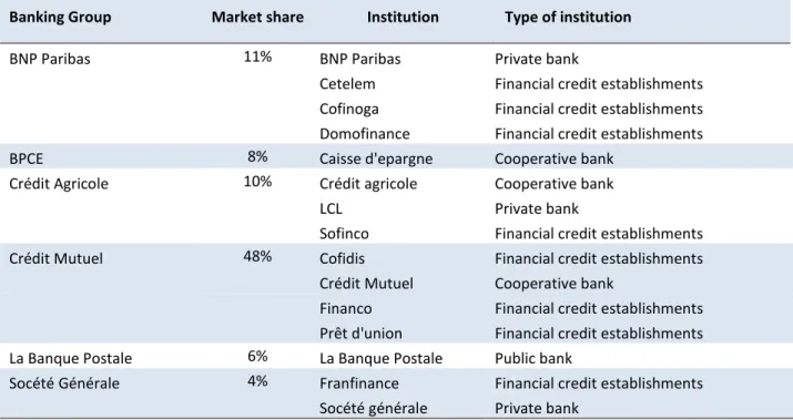
Banks and credit institutions supplied 60% of total consumer credit, with the remaining part being supplied by goods retailers or department stores in tied purchase and a smaller fraction by relatives (Mouillard, 2017). The credit market in France is generally considered to be competitive in that it involves a few large banking groups (which own both retail banking companies and credit institutions) with similar market shares (see Table 1). Banking groups however enjoy some degree of market power, due in particular to relatively high switching costs, which produce a fair amount of product differentiation (Bourdin, 2006; Europe Economics, 2009).

3.2 Data collection

Our dataset consists of a panel of interest rates retrieved from online credit simulators. Most credit institutions in France make such simulators available to prospective borrowers. A simulator typically makes queries about the amount, duration and designation of the desired loan, from which it returns loan terms, including the fixed nominal interest rate, possibly some fees, and the annual percentage yield (taux annuel effectif global), which expresses the yearly cost of the loan. Importantly, simulators have a fairly standardized layout and do not make queries about the applicant’s characteristics nor any specific contractual clauses. The resulting loan-term data are therefore plausibly immune from sorting bias based on applicants’ characteristics unobserved to the lender. They are also immune from issues

5

This share was a historical low, down from 34% in 2008. It was back to 27% in 2018 (Mouillard, 2019).

6 _{Until 2011, home improvements could be included in mortgage loans. This is now only the case for investments}

8 related to collateral, as the simulators do not make any query about wishes regarding the type of guarantee.

Other selection issues may nevertheless be of concern. First, the prospective borrowers that search online may differ from those who remain loyal to their bank, and thus be offered different interest rates. While we cannot control for this, the fact that our interest rates are very close to the effective ones (as we discuss later in Figure 2) suggests it is likely not a major concern. Second, the credit category surveyed is that of personal loans, for which the choice of a designation is non-committal (unlike for crédit affecté attached to a specific designation). As long as loan designations are non-committal, a prospective borrower can always pretend to borrow for the designation that produces the lowest interest rate, so there should be no reason for a lender to differentiate rates by designation. If we do observe differences across designations, it therefore means that lenders exploit some sort of consumer naïveté. While this does not qualitatively affect our hypothesis, it is important to bear in mind.

We designed a web-scraping algorithm that ran such simulators on a weekly basis. This allowed us to assemble a panel dataset of simulated loan terms. We surveyed all credit institutions which, to our knowledge, offered online simulators for household unsecured credit in France during the observation period. This includes 15 institutions which are either the main retailer or some credit subsidiaries of the six main French banking groups, altogether covering 88% of issued loans (Table 1). We operated the algorithm for two years, from January 2015 to October 2016, which produced 93 weeks of data. Each week, for a given institution offering a given designation, the algorithm ran the simulator 108 times, combining 12 different amounts – ranging from 5,000€ to 32,500€, with a step of 2,500€ – and 9 different maturities – ranging from 12 to 108 months, with a step of 12. The data thus produced are 4-tuples of institution, designation, amount and maturity.

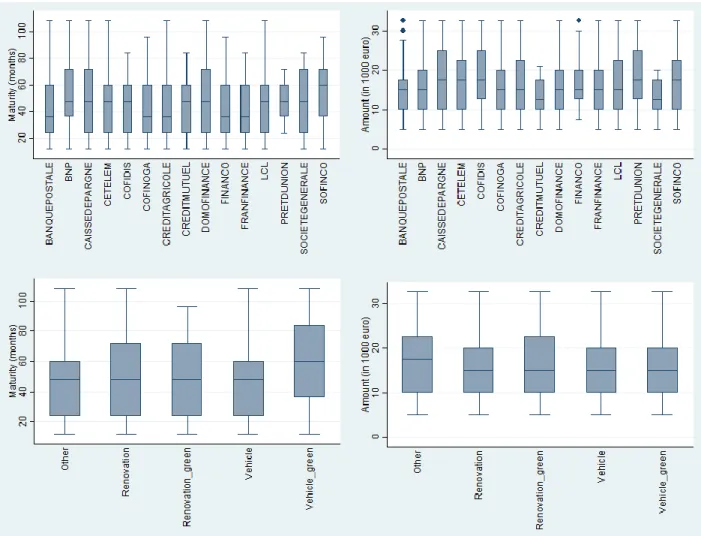
Several sampling issues made our panel dataset unbalanced. First, the menus of designations are specific to each institution, and the number of options each offers varies from 1 to 21 (median 4; mean 7.5). Overall, we recorded 90 different designations, which we grouped into categories, as we will see in the next section. Second, the available ranges of amount and maturity vary as well across institutions. Yet even though sampling was heterogeneous across institutions, this did not introduce a significant bias, as amounts and maturities are very close once averaged per loan category (Figure 1 and Figure 9 in Appendix C).7 The average loan size and maturity over the whole dataset are 16,782€ and 47 months, respectively. Third, some data could not be retrieved for certain institutions on certain weeks, in particular between September and December 2015. This is due to changes in websites that could not be detected early enough to adjust the design of the algorithm – a challenge common in web scraping

7

The higher average maturity associated with vehicle_green in Figure 1 is due to the fact that only one institution – BNP Paribas – offers this designation. Specifically, two features make the difference particularly salient. First, BNP Paribas is the second institution offering the highest average maturities (52.7 months, against 39.7 to 52.8 for other institutions). Second, it offers particularly high maturities for green vehicles (58.4 months on average, against 48.2 to 54.2 for other designations). Whether determined by BNP Paribas’ specific clientele or the configuration of its online simulator, this higher maturity does not introduce any bias in our analysis, though, since we control for both loan amount and maturity in our regressions.

9 (Cavallo and Rigobon, 2016). This gap does not affect our results, since we include time-fixed effects in our panel regressions. Overall, our workable panel dataset comprises 240,962 observations.

Table 1: Characteristics of the institutions surveyed

Banking Group Market share Institution Type of institution BNP Paribas 11% BNP Paribas Private bank

Cetelem Financial credit establishments Cofinoga Financial credit establishments Domofinance Financial credit establishments BPCE 8% Caisse d'epargne Cooperative bank

Crédit Agricole 10% Crédit agricole Cooperative bank

LCL Private bank

Sofinco Financial credit establishments Crédit Mutuel 48% Cofidis Financial credit establishments Crédit Mutuel Cooperative bank

Financo Financial credit establishments Prêt d'union Financial credit establishments La Banque Postale 6% La Banque Postale Public bank

Socété Générale 4% Franfinance Financial credit establishments Socété générale Private bank

Note: Market share estimates were computed by the authors using data from the Banque de France (CEFIT database for 2015). The institutions surveyed cover 88% of the market.

10

Figure 1: Summary statistics of simulated amounts and maturities

3.3 Loan categorization

The number and labelling of options offered by institutions in their menu of loan designations vary widely. After grouping redundant labels, we still handle 90 distinct designations, which are all variants of vehicle loans, home renovation loans, equipment loans, consumption loans, student loans, health loans and cash loans (all representative of the designations reported in Section 2.1).

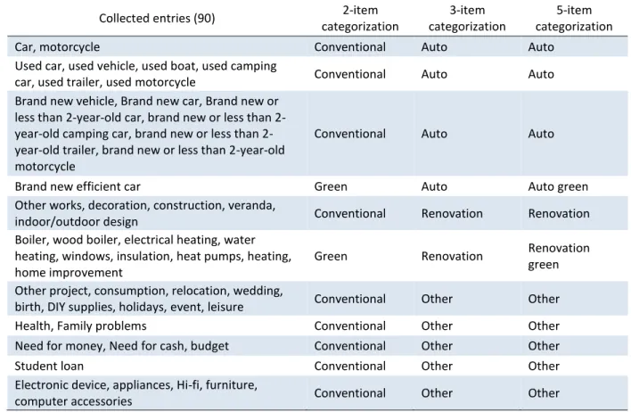
To test the hypotheses stated in Section 2, we group the collected designations into broad categories. Combining the two hypotheses, we are specifically interested in four categories: renovations, green renovations, conventional projects, and green projects. Given the large market share of vehicle projects, we sort this category out of conventional investments. Another motivation for doing so is that one institution makes a distinction between green and conventional vehicles. Our most granular categorization therefore has five items: renovations, green renovations, vehicles, green vehicles, and others. To test the two hypotheses separately, we also consider two more aggregate categorizations: one that groups all green categories on the one hand, all conventional categories on the other; another that groups all renovation categories on the one hand, all vehicle categories on the other. The three workable categorizations are detailed in Table 2. Overall, eleven institutions offer both vehicle and

11 renovation loans; four institutions – Cetelem, Domofinance, Financo and Prêt d'Union – offer both green and conventional retrofits; and one – BNP Paribas – offers both green and conventional vehicles.

Table 2: Categorization of loan designations

Collected entries (90) 2-item categorization

3-item categorization

5-item categorization Car, motorcycle Conventional Auto Auto

Used car, used vehicle, used boat, used camping

car, used trailer, used motorcycle Conventional Auto Auto Brand new vehicle, Brand new car, Brand new or

less than year-old car, brand new or less than year-old camping car, brand new or less than 2-year-old trailer, brand new or less than 2-2-year-old motorcycle

Conventional Auto Auto

Brand new efficient car Green Auto Auto green Other works, decoration, construction, veranda,

indoor/outdoor design Conventional Renovation Renovation Boiler, wood boiler, electrical heating, water

heating, windows, insulation, heat pumps, heating, home improvement

Green Renovation Renovation green Other project, consumption, relocation, wedding,

birth, DIY supplies, holidays, event, leisure Conventional Other Other Health, Family problems Conventional Other Other Need for money, Need for cash, budget Conventional Other Other Student loan Conventional Other Other Electronic device, appliances, Hi-fi, furniture,

computer accessories Conventional Other Other

The categorization procedure is crucial. Most collected designation labels are unambiguous and their allocation to the appropriate category is straightforward. This is not quite the case for green and conventional retrofits, which are nevertheless central to our analysis. Making a distinction between the two requires careful interpretation of the labels. Our approach is to allocate to the green retrofit category those retrofit labels that likely reduce the energy consumption of a household. This essentially includes measures on the building envelope and the space and water heating systems. As a robustness check, we subject this categorization to placebo tests and conclude that it is meaningful (see Section 6.2). Moreover, we also play around the vehicle designation, in particular by adding ‘new vehicles’ to the ‘green’ category. This allows us to have a ‘green category’ not limited to one bank. Here again, the variants considered confirm the robustness of our results (see Section 6.3). Note that the ‘green’ information contained in the different menus is too coarse – in particular for automobiles – to match the detail of eligibility requirements to subsidy programs. It is therefore reasonable to consider that the subsidy programs discussed in Appendix A do not directly interfere with the loans studied here.

12

3.4 Descriptive statistics

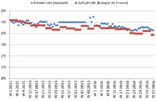
We focus below on the average percentage yield (APY), which represents the monthly price of a loan, including fees. The weekly interest rates vary within 1.5 percentage point on a weighted average basis. An obvious concern with our posted data is the accuracy with which they approximate actual data. Comparing the trend of the average interest rate in our dataset, weighted by the market share of the corresponding banking group, to that of issued loans provided by the Banque de France,8 we find a positive spread on 73 weeks out of 93 (Figure 2). The mean percentage error over the whole period is 6.0% (mean absolute percentage error: 6.9%; standard error 4.7%), or a 0.3 percentage point. Such a relatively low error lends external validity to our data. Moreover, the fact that the rates on issued loans are almost systematically below posted rates can be interpreted as preliminary evidence of the negotiation process lenders and borrowers are known to engage in (see Allen et al., 2014a,b, for evidence from Canada).

Figure 2: Comparison between posted and actual interest rates

The interest rates posted by credit institutions exhibit some dispersion across space and time. On average, the surveyed institutions update their interest rates every seven weeks and exhibit a coefficient of variation on interest rate of 33% (Figure 3, red square). As we will see later in regressions, dispersion is further substantiated by strong variations in average interest rates across banks. This illustrates the fact that, despite operating in a highly competitive market, institutions adopt heterogeneous pricing strategies (cf. Section 3.1). 8 http://webstat.banque-france.fr/fr/browseChart.do?node=5385583&sortByView454=468&SERIES_KEY=MIR1.M.FR.B.A2B.A.R.A.2254U6.E UR.N&SERIES_KEY=MIR1.M.FR.B.A2B.A.R.A.2250U6.EUR.N

13

Figure 3: Dispersion of average interest rates across space and time, by institution

Looking at the time series of weighted averages of interest rate, some clear, yet unstable, differences exist between categories (Figure 4). The two green categories tend to be associated with lower interest rates. In particular, the average interest rate on green vehicles – which we recall are offered by BNP Paribas only – drops significantly early in 2016.

Figure 4: Time series of average spread (in percentage points), by category

Another look suggests that the interest rates averaged by maturity co-move to a large extent (Figure 5). Yet 12-month loans exhibit a peculiar pattern, with an interest rate decreasing more markedly than that of other maturities from early 2016 onwards. This coincides with an increase in deposits of €154 billion between 2015 and 2016 induced by quantitative easing by the European Central Bank (ACPR, 2016). It is

14 likely that banks offered particularly low interest rates on short-term loans to recycle these vast amounts of cash money.

Figure 5: Time series of average spread (in percentage point), by maturity (in months)

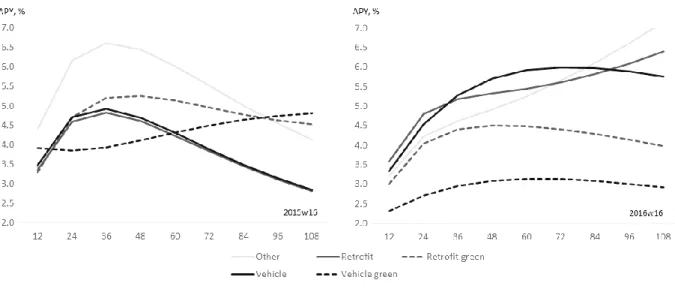
Figure 6 sheds light on the interaction between these phenomena through the market yield curve, which illustrates how interest rates vary with maturities. We constructed the yield curves for each category using the Nelson-Siegel-Svensson model (Nelson and Siegel, 1987) and estimated them at two points in time: week 16 in 2015 and week 16 in 2016.

Figure 6: Empirical yield curves at two points in time, by category (months on horizontal axis)

We observe that all categories (except green vehicles) exhibited a bell-shaped curve in 2015, with a negative slope for high maturities. In 2016, expectations went back to normal, with a more usual positive

15 slope for conventional categories. The two green categories however underwent a downward shift, which suggests recognition of the lower risk associated with green projects. These observations call for a separate analysis of interest rates across maturities (12-month versus higher maturities) and over time (2015 versus 2016).

4 Econometric model

Our goal is to make inference on how credit institutions perceive the risks associated with different loan designations. We consider the spread 𝑠 between the posted interest rate 𝑖 (measured by the APY) in our dataset and the spot yield of the government bond 𝑏 of the same maturity:9

𝑠𝑘𝑎𝑚𝑡𝑐 = 𝑖𝑘𝑎𝑚𝑡𝑐− 𝑏𝑚𝑡,

where 𝑘 ∈ {1, … ,15} denotes the credit institution, 𝑎 ∈ {5000,7500, … ,32500} the amount simulated in euros, 𝑚 ∈ {12,24, … ,108} the maturity of the loan in months, 𝑐 one category within one of the three retained categorization and 𝑡 the week on which the loan was simulated. Regressing the spread instead of using government bonds to explain the interest rate allows us to address potential endogeneity problems between the two. It moreover allows us to focus on the bank margin, which is the part of the interest rate most affected by loan designations. Note that, as government bonds carried negative yields over the period, the spread is generally larger than the associated interest rate.

We consider a parsimonious model that expresses the spread as a linear combination of the following determinants:

𝑠_{𝑘𝑎𝑚𝑐𝑡} = 𝛼₀+ 𝛼₁𝐿_𝑎𝑚+ 𝛼₂𝐼_𝑘+ 𝛼₃𝑇_𝑡𝐼_𝑘+ 𝛽_𝑐𝐷_𝑐+ 𝜀_{𝑘𝑎𝑚𝑐𝑡},

where: 𝐿𝑎𝑚 is a vector of loan characteristics, including the duration of the loan, its square, and the

amount borrowed; 𝐼𝑘 is a vector of institution fixed effects; 𝑇𝑡 is a vector of time fixed effects; and 𝐷𝑐 is a

vector of project categories. Through the institution fixed effect, we assume that different lenders adopt different pricing strategies, depending on their client portfolio, size or capitalization. The product 𝑇𝑡𝐼𝑘

captures institutions’ individual responses to changes in the macroeconomic and financial environment and helps address autocorrelation in the residuals.10 The associated coefficient 𝛼3 can be interpreted as

the additional effect of a particular institution for a particular loan category with respect to the average effect of that institution 𝛼2 and the average effect of that loan category 𝛽𝑐.11

9

For the French government bond yields, we use the data on the observed yields for tradable maturities and inferred rates for nontradable maturities, as given by the ECB (Source: ECB, Data Source in SDW: Government bond, nominal, all issuers whose rating is triple A - Svensson model - continuous compounding - yield error minimization - Yield curve spot rate - Euro, provided by ECB).

10

Classical heteroscedasticity tests do not apply to regressions with weighted observations. Nevertheless, visual inspection of residuals suggests little heteroscedasticity or autocorrelation.

11

The institution and institution*time fixed effects allow us to deal with the cross-institution correlation and the autocorrelation of the error terms. This increases the precision of our estimates. One legitimate question is whether we should cluster errors by designation or institution to account for intra-institution correlation. Based on Abadie et al. (2017), we see two reasons for not doing so. First, the authors provide theoretical and experimental

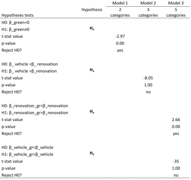
16 The coefficients 𝛽𝑐 associated with loan categories are our main estimates of interest. We subject them

to 𝑡-tests in order to assess the hypotheses stated in Section 2, which we statistically reformulate as follows:

Ha: 𝛽₁𝑔𝑟𝑒𝑒𝑛 < 𝛽1𝑐𝑜𝑛𝑣𝑒𝑛𝑡𝑖𝑜𝑛𝑎𝑙

Hb : 𝛽1𝑣𝑒ℎ𝑖𝑐𝑙𝑒≤ 𝛽1𝑟𝑒𝑡𝑟𝑜𝑓𝑖𝑡

We test Ha with the two-item categorization, Hb with the three-item categorization and examine the

interaction of the two hypotheses with the five-item categorization. To ensure representativeness of our loan sample, we assign weights to our observations proportional to the share of the corresponding banking group in the French market for personal consumer credit (Table 1).12 We further assign uniform weights to all subsidiaries within a banking group. We do not further assign weights by projects for lack of supporting data.

5 Estimation results

5.1 General effect of loan designation

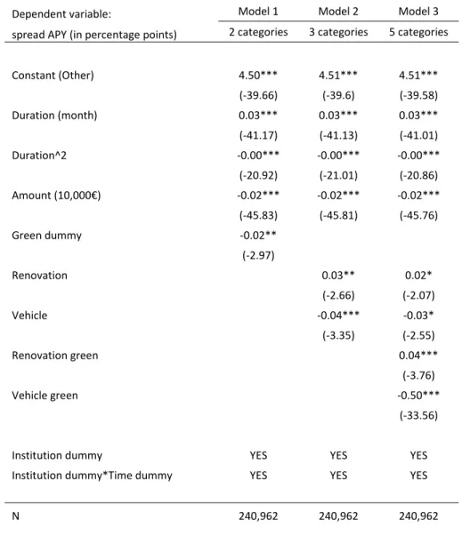
We estimate three variants of the model with ordinary least squares (OLS): model 1 uses the two-item categorization; model 2 uses the three-item categorization; model 3 uses the five-item categorization (Table 3). As expected, the spread is positively associated with the duration, though at a slightly decreasing rate. An additional year increases the spread by about 0.4 percentage point. In contrast, the amount has a very small, negative effect on the spread.

The comparison of projects dummies across models suggests that green projects are priced below conventional projects (model 1) and that vehicle projects are priced below renovation projects (model 2). These results are statistically significant at conventional levels and confirmed by 𝑡-tests (Table 4), but small in magnitude. Interacting the two dimensions in model 3, we see that the former result does not apply to renovations and is in fact driven by the strong discount observed on green vehicles, which we recall is attributable to one institution. Again, these results are statistically significant and confirmed by 𝑡-tests. The polarity of the difference in marginal prices for vehicles and home renovation is consistent with either the moral hazard or surplus-extracting screening hypotheses.

When it comes to the green dimension, we find that it goes in opposite directions for vehicles and renovations. While efficient pricing seems to apply to green vehicles, our results suggest that home energy efficiency is subject to a double energy efficiency gap: the first because renovation projects carry

evidence that variance adjustment can lead to overestimation of the standard errors if the number of clusters in the sample is close to the total number of clusters in the population. As our dataset covers 88% of the market, the omitted fraction of the population is unlikely to form a large number of clusters. Second, the authors point out that heterogeneity in the treatment effects is a necessary condition for clustering adjustment. In our sample, observations get no treatment (or, put differently, treatment is homogeneous across observations).

12

Weighting here is indispensable to accurately describe the underlying population of loans (see Solon et al, 2015).

13 _{The standard errors reported in all regression tables tend to be very small – typically 0.00. We therefore report}

17 higher interest rates; the second because within this category, the green attribute further increases the interest rate. The latter effect may be due to lenders anticipating information asymmetries about the quality of home energy retrofits (Giraudet et al., 2018b), as discussed in Section 2.

To put these numbers in perspective, let us consider average loans of €15,000 borrowed over 48 months. The differences in interest rates we estimate for different purposes are equivalent to the following differences in the total cost of such loans: €50 between home retrofits and automobiles; €14 between a green and a conventional retrofit; -€333 between a green and a conventional automobile. These differences are small relative to the monetary savings generated by energy efficiency improvements, which typically amount to €300 annually – considering 20% efficiency improvement on an annual expenditure of €1,500 for both heating and transportation14 – hence €1,200 over the duration of a 48-month loan.

Table 3: OLS estimates of the baseline regression

Dependent variable: Model 1 Model 2 Model 3

spread APY (in percentage points) 2 categories 3 categories 5 categories

Constant (Other) 4.50*** 4.51*** 4.51*** (-39.66) (-39.6) (-39.58) Duration (month) 0.03*** 0.03*** 0.03*** (-41.17) (-41.13) (-41.01) Duration^2 -0.00*** -0.00*** -0.00*** (-20.92) (-21.01) (-20.86) Amount (10,000€) -0.02*** -0.02*** -0.02*** (-45.83) (-45.81) (-45.76) Green dummy -0.02** (-2.97) Renovation 0.03** 0.02* (-2.66) (-2.07) Vehicle -0.04*** -0.03* (-3.35) (-2.55) Renovation green 0.04*** (-3.76) Vehicle green -0.50*** (-33.56)

Institution dummy YES YES YES

Institution dummy*Time dummy YES YES YES

N 240,962 240,962 240,962

14 _{In 2010, French households annually spent €2,300 on energy, split roughly evenly into housing (57%) and}

18

R-sq 0.414 0.415 0.415

adj. R-sq 0.412 0.412 0.413

t-statistics in parentheses

* p<0.05, ** p<0.01, *** p<0.001

Table 4: Statistical tests on the baseline regression

Model 1 Model 2 Model 3

Hypotheses tests Hypothesis 2 categories 3 categories 5 categories H0: β_green=0 H1: β_green≠0 Ha t-stat value -2.97 p-value 0.00 Reject H0? yes H0: β_ vehicle <β_ renovation H1: β_ vehicle >β_renovation Ha t-stat value -8.05 p-value 1.00 Reject H0? no H0: β_renovation_gr<β_renovation H1: β_renovation_gr>β_renovation Ha t-stat value 2.66 p-value 0.00 Reject H0? yes H0: β_vehicle_gr<β_vehicle H1: β_vehicle_gr>β_vehicle Ha t-stat value -35 p-value 1.00 Reject H0? no

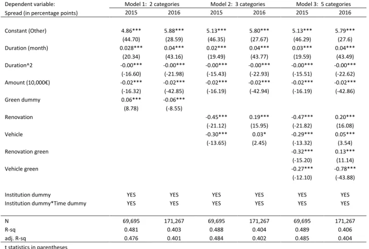
5.2 Effects by year of sample

Motivated by the changes observed in the time series split by categories (Figure 4) and changes in the yield curve (Figure 6), we estimate the different models on year subsamples (Table 5). The coefficients associated with duration indicate a steeper yield curve in 2016. The green discount observed over the period is only effective in 2016; conversely, in 2015, green projects carry a higher interest rate (model 1). Likewise, the ranking observed over the period between renovation and vehicle projects only applies to 2016 and is reversed in 2015 (model 2). The change in the merit order of the five categories observed in 2016 is consistent with an interaction between these two shifts (model 3). Again, all results are

19 statistically significant and confirmed by 𝑡-tests. This leads us to the conclusion that the double energy efficiency gap is not consistent over the period: in 2015, only its first dimension applies, whereas in 2016, only its second dimension applies. In other words, the market seems to increasingly recognize the lower risk associated with green projects; meanwhile, it charges increasingly higher interest rates for renovation projects than for vehicles. The first effect is consistent with the notion that financial agents increasingly value environmental aspects, as recently documented by An and Pivo (2018) in the US market for commercial mortgages and Karpf and Mandel (2018) in the US market for municipal bonds.

Statistical tests not displayed here confirm the results. More generally, since the standard errors of the estimates are very small, the differences between the estimated coefficients are always statistically significant, so the validity of the hypotheses can be verified simply by comparing the values of the corresponding coefficients.

Table 5: Evolution of the effects

Dependent variable: Model 1: 2 categories Model 2: 3 categories Model 3: 5 categories

Spread (in percentage points) 2015 2016 2015 2016 2015 2016

Constant (Other) 4.86*** 5.88*** 5.13*** 5.80*** 5.13*** 5.79*** (44.70) (28.59) (46.35) (27.67) (46.29) (27.6) Duration (month) 0.028*** 0.04*** 0.02*** 0.04*** 0.03*** 0.04*** (20.34) (43.16) (19.49) (43.77) (19.59) (43.49) Duration^2 -0.00*** -0.00*** -0.00*** -0.00*** -0.00*** -0.00*** (-16.60) (-21.98) (-15.43) (-22.93) (-15.51) (-22.62) Amount (10,000€) -0.02*** -0.02*** -0.02*** -0.02*** -0.02*** -0.02*** (-16.32) (-42.85) (-16.19) (-42.94) (-16.19) (-42.86) Green dummy 0.06*** -0.06*** (8.78) (-8.55) Renovation -0.45*** 0.19*** -0.47*** 0.20*** (-21.12) (15.95) (-21.82) (16.08) Vehicle -0.30*** 0.03* -0.29*** 0.05*** (-13.65) (2.45) (-13.32) (3.54) Renovation green -0.32*** 0.13*** (-15.20) (11.14) Vehicle green -0.27*** -0.78*** (-12.10) (-43.88)

Institution dummy YES YES YES YES YES YES

Institution dummy*Time dummy YES YES YES YES YES YES

N 69,695 171,267 69,695 171,267 69,695 171,267 R-sq 0.481 0.403 0.488 0.404 0.489 0.406 adj. R-sq 0.476 0.401 0.484 0.402 0.485 0.404 t statistics in parentheses * p<0.05, ** p<0.01, *** p<0.001

5.3 Effects by loan maturity

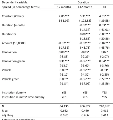
Motivated by the changes observed in the time series split by maturities (Figure 5), we estimate model 3 on duration subsamples, considering separately 12-month loans and loans with longer duration (Table 6). (See Appendix B for further disaggregation of the regressions.) The ranking of categories for 12-month loans conforms that observed at the aggregate level. When considering loans with longer

20 duration, this ranking changes in one important respect: green renovations are charged lower interest rates than conventional renovations. In other words, lenders seem to perceive green retrofits as riskier investments when financed by a short-term loan than when financed by a long-term loan. Further regressions on both year and maturity subsamples suggest that this phenomenon essentially occurred in 2016.

Table 6: Comparison of short-term and long-term effects

Dependent variable: Duration

Spread (in percentage terms) 12 months >12 month all

Constant (Other) 2.85*** 5.31*** 4.51*** (-51.02) (-123.82) (-39.58) Duration (month) -0.02*** 0.03*** (-14.37) (-41.01) Duration^2 0.00*** -0.00*** (-18.83) (-20.86) Amount (10,000€) -0.02*** -0.02*** -0.02*** (-17.56) (-43.78) (-45.76) Renovation 0.08*** -0.03* 0.02* (-3.83) (-2.29) (-2.07) Renovation green 0.31*** -0.06*** 0.04*** (-13.2) (-5.60) (-3.76) Vehicle 0.08** -0.05*** -0.03* (-3.12) (-4.32) (-2.55) Vehicle green 0.05** -0.56*** -0.50*** (-1.84) (-37.02) (-33.56)

Institution dummy YES YES YES

Institution dummy*Time dummy YES YES YES

N 34,135 206,827 240,962 R-sq 0.662 0.469 0.415 adj. R-sq 0.652 0.466 0.413 t statistics in parentheses * p<0.05, ** p<0.01, *** p<0.001

5.4 Effects by lending institution

We run an alternative specification of model 3 with an additional interaction term 𝐷𝑐𝐼𝑘 meant to capture

the idiosyncratic way in which institutions price the risk associated with loan designations, as compared to the market. The results are displayed in Table 7. Generally speaking, Cofidis, Credit Mutuel, Société Générale and Cofinoga post the highest interest rates while LCL, BNP, Caisse d'Epargne and Cetelem post the lowest rates (column 1). The specific way in which an institution values a project category is given by the sum of the institution coefficient in the first column and the appropriate coefficient in the institution-category matrix. Thus estimated, the institutions’ pricing strategies appear highly heterogeneous. The difference in average rates across banks is as large as 5 percentage points, with Cofidis and LCL offering the highest and lowest rates, respectively, suggesting that they target different customers. Among the institutions making a distinction between green and conventional renovations, Domofinance, Financo

21 and Prêt d’union offer lower interest rates for the former, while Cetelem adopts the opposite strategy. On average, only Financo prices green renovation loans below conventional renovation loans, and only Caisse d’Epargne, Cofidis, Cofinoga and Credit Mutuel price renovation loans below vehicle loans.

We then analyze whether holding a green certification affects the pricing behavior of lenders. Three certifications exist in France: Transition énergétique et écologique pour le climat (TEEC15) awarded by the Ministry of Finance since December 2015; Investissement socialement responsable (ISR16) awarded by the Ministry of Finance since September 2015 and the Principles for Responsible Investment (PRI17) launched in April 2006 by the United Nations for corporations worldwide. While the TEEC and ISR labels are awarded after an extensive external audit, PRI consists of a list of recommendations that a signatory commits to follow. In general, these certifications do not involve ex post verification. We assume that lenders apply their guiding principles to their personal loans, at least for advertising purposes.

Table 7: Effects by loan type and lenders

Loan type FE Institution FE Renovation Renovation Green Vehicle Vehicle Green

Average loan-type effect -0.32*** -0.00*** -0.41*** -0.77***

Loan FE BNP -0.81*** 0.01*** -0.62** -0.77*** CAISSE D'EPARGNE -1.09*** 1.34*** 1.72*** CETELEM -0.98*** 0.26*** 0.44*** -0.41*** COFIDIS 2.07*** -0.08** 0.03*** COFINOGA 0.45** -0.62** -0.41*** CREDIT AGRICOLE -0.06 0.07*** -0.20* CREDIT MUTUEL 0.82*** -3.60*** -0.93*** DOMOFINANCE -0.46*** -0.66*** -0.59*** FINANCO -0.05 -0.41 -0.55*** -0.78*** FRANFINANCE -0.87*** 0.14*** LCL -2.81*** 0.89*** PRET D'UNION -0.35** -0.00*** 0.00*** SOCIETE GENERALE 0.52** SOFINCO -0.51** 1.48***

Note: The average interest rate for “Other” loans offered by Banque Postale is taken as a basis for comparison and is omitted in this table. Banque Postale did not offer green loans during the period of observation.

Table 8 displays the dates of certification award to at least one fund of a banking group. For our analysis, we consider a banking group to be green-certified if it was awarded at least one certification by the beginning of 2015. 15 https://www.ecologique-solidaire.gouv.fr/label-transition-energetique-et-ecologique-climat 16 _{https://www.lelabelisr.fr/quest-ce-que-isr/} 17 https://www.unpri.org/

22

Table 8: Green certifications

Date of certification award At least one certification by

the beginning of 2015

PRI TEEC ISR

BNP 27 April 2006 1 September 2015 YES

BPCE NO

Credit Agricole 08 March 2010 YES

Credit Mutuel

14 September

2012 1 June 2017 after 1 September 2016 YES

LBP

20 January

2009 6 June 2017 13 September 2017 YES

Societe generale NO

We run the baseline regression with five loan categories on the sample of green-certified lenders and non-certified ones. The results are presented in Table 9.

Table 9: Estimation results for green-certified and non-certified lenders

Dependent variable Green label

spread No Yes Constant 4.11*** 4.28*** (43.46) (79.21) Duration (months) 0.04*** 0.035*** (19.28) (36.83) Duration^2 -0.00*** -0.00*** (-11.06) (-20.76) Amount (10,000€) -0.05*** -0.02*** (-24.28) (-30.14) Dummy Retrofit 1.08*** -0.20*** (33.88) (-15.06)

Dummy Retrofit Green -0.82***

(-68.65)

Dummy Vehicle 1.31*** -0.31***

(41.17) (-25.54)

Dummy Vehicle Green -1.65***

(-95.33)

Time fixed effects YES YES

N 22,213 218,749

R-sq 0.212 0.138

adj. R-sq 0.209 0.138

t statistics in parentheses

23 Green loan options turn out to be only offered by green-certified lenders (BNP Paribas, Cetelem, Domofinance, Financo and Prêt d’union belonging to the green-certified groups BNP Paribas and Crédit Mutuel). The regression confirms that their pricing behavior is responsible for the green discount previously found in the full sample: indeed, green-certified lenders tend to assign lower rates to green projects, for renovations and even more so for vehicles. The regressions nevertheless suggest that the two groups adopt opposite pricing strategies with respect to Hypothesis 2. Non-certified lenders set lower rates for renovation projects, while green-certified lenders do the opposite, even more so for green projects.

6 Robustness checks

6.1 Macroeconomic and financial controls

We substitute a set of macroeconomic and financial variables for time fixed effects and examine how it affects the values of the estimated coefficients of loan categories. We estimate the following model:

𝑠_{𝑘𝑎𝑚𝑐𝑡} = 𝛼₀+ 𝛼₁𝐿_𝑎𝑚+ 𝛼₂𝐼_𝑘+ 𝛼₃𝑀_𝑀

𝑡+ 𝛼3𝐹𝐹𝑡+ 𝛽𝑐𝐷𝑐+ 𝜀𝑘𝑎𝑚𝑐𝑡,

where 𝑀𝑡 is a vector of macroeconomic variables, 𝐹𝑡 a vector of financial variables, and all other

variables are those defined in the previous model. Macroeconomic controls include: the inflation rate, as measured by the harmonized index of consumer prices; the unemployment rate, which approximates the phase of the business cycle; the interest rate on one-year government bonds in the Euro area, which captures the quantitative easing the European Central Bank (ECB) engaged in during the period. Financial controls include: the spread between the return on the CAC40 index and the interest rate on one-year government bonds, which approximates the volatility of the stock market; the stress index provided by the ECB, which approximates the volatility in the bond market;18 and investors’ expectations, as measured by the slope of the yield difference between ten-year and one-year government bonds.

These substitutions do not qualitatively alter the results of the baseline model and preserve the ranking between interest rates associated with different project categories (Table 10). Macroeconomic and financial factors explain a very modest part of the variation of the spread, which is consistent with previous findings (Gambacorta, 2008). This finding is not surprising, as macro factors exhibited little variation during the period. Unemployment stands out as the only added control with a statistically significant effect. Its negative sign lends support to our hypothesis that surplus extraction plays an important role in loan pricing. Indeed, higher unemployment implies depressed demand, to which lenders motivated by surplus extraction may respond with lower interest rate margins.

Despite being non-significant, estimates for the other variables have the expected polarity. Quantitative easing has a positive effect, suggesting that institutions benefited from a loosening of the monetary policy, possibly at the expense of consumers. Inflation too has a positive effect, suggesting that cost

18

Euro area (changing composition), Stress subindice - Bond Market - realised volatility of the German 10-year benchmark government bond index, yield spread between A-rated non-financial corporations and government bonds (7-year maturity bracket), and 10-year interest rate swap spread, Contribution.

24 pass-through is affected by some degree of market power. Higher risks in the equity market – as approximated by the two volatility indices – increase the spread, suggesting that lenders transfer part of the portfolio risks to their customers. The impact of the yield curve slope is positive, suggesting that optimistic expectations are associated with a higher demand for consumer loans.

Table 10: Effect of macroeconomic and financial controls

Dependent variable Baseline model with controls for

APY spread (in percentage points)

Baseline model Macro factors Financial factors Macro and financial factors Constant (Other) 4.51*** 6.79*** -5.22 -5.13 (-39.58) (-6.94) (-0.00) (-0.00) Duration (month) 0.03*** 0.03*** 0.03*** 0.03*** (-41.01) (-41.02) (-41.01) (-41.02) Duration^2 -0.00*** -0.00*** -0.00*** -0.00*** (-20.86) (-20.86) (-20.86) (-20.86) Amount (10,000€) -0.02*** -0.02*** -0.02*** -0.02*** (-45.76) (-45.75) (-45.76) (-45.75) Dummy Retrofit 0.02* 0.02* 0.02* 0.02* (-2.07) (-1.88) (-2.07) (-1.88)

Dummy Retrofit Green 0.04*** 0.04*** 0.04*** 0.04***

(-3.76) (-3.63) (-3.76) (-3.63)

Dummy Vehicle -0.03* -0.03** -0.03* -0.03**

(-2.55) (-2.83) (-2.55) (-2.83)

Dummy Vehicle Green -0.50*** -0.50*** -0.50*** -0.50***

(-33.56) (-33.78) (-33.56) (-33.78) One-year bonds 11.33 -1.27 (0.34) (-1.23) Price index 0.20 -0.03 (0.97) (-0.68) Unemployment -0.11*** -0.11*** (-6.29) (-6.29) CAC40 1.87 2.17 (-0.65) (0.65) Stress index 15.84 17.02 (1.03) (-0.65)

Yield curve slope 0.69 -0.07

(0.49) (-0.39) N 240,962 240,962 240,962 240,962 R-sq 0.415 0.416 0.415 0.416 adj. R-sq 0.413 0.413 0.413 0.413 t-statistics in parentheses * p<0.05. ** p<0.01. *** p<0.001

25

6.2 Placebo tests on retrofit designations

As stated in Section 3.3, we build our own categorization out of the 90 distinct designations collected by the algorithm. While most designations labels are so clear as to be categorized in a straightforward manner, green-renovation labels are subject to interpretation. We conduct two placebo tests to examine the relevance of our categorization in general, and that of the green-renovation category in particular.

In the first placebo test, we randomly assign each of the 90 designations to one out of five arbitrary categories, following a uniform distribution. We then produce OLS estimates of model 3 with these categories, simply labelled 1 to 5. We repeat this procedure 1,000 times. Figure 7 displays the distribution of estimated coefficients for all categories. Table 11 displays the mean of obtained coefficients and 𝑝-values. The table confirms that the coefficients estimated for arbitrary categories are centered around zero. The mean of the 𝑝-value is 0.5 and it is uniformly distributed, as it should be under the null hypothesis that the value of each of the coefficients is zero. The results lead us to the conclusion that our five-item categorization is meaningful.

Figure 7: Placebo test on all categories

Table 11: Placebo test on all categories

Cj=2 Cj=3 Cj=4 Cj=5 Average β1 0.00 0.00 0.00 0.00 Average σβ1 0.01 0.01 0.01 0.01 Average p-value 0.50 0.50 0.51 0.50

26 In the second placebo test, we restrict the procedure to those designations which initially fell in either renovation or green renovation categories. We randomly assign those designations to two arbitrary categories while maintaining other designations in their initial category (vehicle, green vehicle and other). We then estimate model 3 and repeat the procedure 1,000 times. The distributions of estimated coefficients appear much narrower for the two vehicle categories than for the two arbitrary renovation categories (Figure 8). The latter are moreover centered around the same value. The mean 𝑝-value of 0 indicates that, on average, the null hypothesis on the insignificance of the coefficients is rejected (Table 12). Moreover, the probability distribution of the 𝑝-value is not uniform but has a bell shape skewed towards zero, as it should when the null is rejected. This indicates that, irrespective of the green attribute, the retrofit category has a significant impact on the spread. A statistical test fails to reject the null hypothesis that estimated coefficients for the two arbitrary categories are equal (F(1,239939)=0.16; Prob>F=0.6901), as the two placebo categories are now indistinguishable. However, they are different from our baseline estimates obtained with our categorization (F(1,239939)=9.03;Prob>F=0.0001), thus implying that our categorization of conventional and green renovations is also meaningful.

Figure 8: Placebo test on renovation categories Table 12: Placebo test on renovation categories

Renovation 1 Renovation 2 Vehicle Vehicle green

Average β1 0.03 0.03 -0.03 -0.51

Average σβ1 0.01 0.01 0.01 0.02

Average p-value 0.00 0.00 0.00 0.00

27

6.3 Vehicle designations

To address potential concerns raised by the fact that our ‘green vehicle’ cateogory rests on only one institution, we play around the categorization of vehicles. We rely on the fact that differences in energy efficiency may also arise between two types of vehicles collected in our dataset: new and second-hand ones. We therefore consider three new groups – new vehicles, second-hand vehicles, and unspecified vehicles – and use them (together with BNP Paribas’ green cars) to build three alternative specifications:

 In Variant 1, we assign new vehicles and BNP Paribas’ green cars to ‘green vehicles’ and second-hand vehicles to ‘conventional vehicles.’ We do not assign unspecified vehicles to any category;

 In Variant 2, we build on variant 1 and add unspecified vehicles to the ‘conventional vehicle’ category;

 In Variant 3, we build on variant 1 and add unspecified vehicles to the ‘green vehicle’ category.

Note that these alternatives are likely to affect not only regressions with the 5-item categorization, but also those with 2-item and 3-item categorizations. Note also that Variant 3 is somewhat of a lure meant to annihilate any green effect.

The estimates provided in Table 13 lend further support to our results. Variant 1 confirms that the difference between new and second-hand cars (presumably associated with differing degrees of energy efficiency) leads to differences in interest rates consistent with those established between truly green and conventional cars. The pricing pattern is no longer specific to BNP and now includes five more institutions offering a ‘green vehicle’ option in their simulator – Banque postale, Cetelem, Cofinoga, Financo and Prêt d’union. Variant 2 confirms these results, though estimates are smaller in magnitude, as is expected by the fact that adding otherwise specified cars to the conventional category somehow dilutes the effect. The screening effect of conventional vehicles vs retrofits also disappears. Variant 3 reverses the green effect (i.e., green vehicles are associated with higher interest rates), which is what this lure is intended to do if the estimates are robust.