Translation and scale invariants of Tchebichef moments

HAL Id: inserm-00139337

https://www.hal.inserm.fr/inserm-00139337

Submitted on 30 Mar 2007

HAL is a multi-disciplinary open access archive for the deposit and dissemination of sci-entific research documents, whether they are pub-lished or not. The documents may come from teaching and research institutions in France or

L’archive ouverte pluridisciplinaire HAL, est destinée au dépôt et à la diffusion de documents scientifiques de niveau recherche, publiés ou non, émanant des établissements d’enseignement et de recherche français ou étrangers, des laboratoires

Translation and scale invariants of Tchebichef moments

Hongqing Zhu, Huazhong Shu, Ting Xia, Limin Luo, Jean-Louis Coatrieux

To cite this version:

Hongqing Zhu, Huazhong Shu, Ting Xia, Limin Luo, Jean-Louis Coatrieux. Translation and scale invariants of Tchebichef moments. Pattern Recognition, Elsevier, 2007, 40 (9), pp.2530-2542. �10.1016/j.patcog.2006.12.003�. �inserm-00139337�

Translation and Scale Invariants of Tchebichef Moments

Hongqing Zhua, Huazhong Shua, c, Ting Xiaa, Limin Luoa, c, Jean Louis Coatrieuxb, c

a

Lab. of Image Science and Technology, Department of Computer Science and Engineering, Southeast University, 210096 Nanjing, People’s Republic of China

b

Laboratoire Traitement du Signal et de l’Image, INSERM U642, Université de Rennes I , 35042 Rennes, France

c

Centre de Recherche en Information Biomédicale Sino-français (CRIBs)

HAL author manuscript inserm-00139337, version 1

HAL author manuscript

Abstract⎯Discrete orthogonal moments such as Tchebichef moments have been successfully used in the field of image analysis. However, the invariance property of these moments has not been studied mainly due to the complexity of the problem. Conventionally, the translation and scale invariant functions of Tchebichef moments can be obtained either by normalizing the image or by expressing them as a linear combination of the corresponding invariants of geometric moments. In this paper, we present a new approach that is directly based on Tchebichef polynomials to derive the translation and scale invariants of Tchebichef moments. Both derived invariants are unchanged under image translation and scale transformation. The performance of the proposed descriptors is evaluated using a set of binary characters. Examples of using the Tchebichef moments invariants as pattern features for pattern classification are also provided.

Keywords: Discrete orthogonal moments; Tchebichef polynomials; Translation and scale invariants;

Pattern classification; Image normalization

1. Introduction

Since Hu [1] first introduced the moment invariant, moments and moment functions have been widely used in the fields of image analysis and pattern recognition [2-8]. Hu’s moment descriptors are invariant with respect to translation, scale and rotation of the image. However, the kernel function of geometric moments of order (p + q), p q

pq(x,y)=x y

ψ

, is not orthogonal, thus the geometric moments suffer from

the high degree of information redundancy [9-10], and they are sensitive to noise for higher-order moments. Zernike and Legendre moments were later introduced by Teague [11] who used the corresponding orthogonal polynomials as kernel functions. Another related orthogonal moments, denoted as pseudo-Zernike moments [9], was derived based on the basis set of pseudo-Zernike polynomials. These orthogonal moments have been proved to be less sensitive to image noise as compared to geometric moments, and possess better feature representation ability [12-18].

Recently, the invariance problem of the orthogonal moments has been investigated by several research groups. The translation and scale invariants of Zernike and Legendre moments were achieved by using image normalization method [19-20]. An efficient method for constructing the translation and scale invariants of Zernike and Legendre moments from their corresponding orthogonal polynomials was developed by Chong et al. [21-22]. A similar method was applied to obtain the scale invariants of pseudo-Zernike moments [23]. Both the Zernike and Legendre moments, as well as the pseudo-Zernike moments, are defined as continuous integrals over a domain of normalized coordinates. The computation of these moments requires a coordinate transformation and suitable approximation of the continuous moment’s integrals, leading thus to further computational complexity and discretization error. To overcome the shortcoming of the continuous orthogonal moments, Mukundan et al. proposed a set of discrete orthogonal moment functions based on the discrete Tchebichef polynomials [24]. Another new set of discrete orthogonal moment functions based on the discrete Krawtchouk polynomials was presented by Yap et al. [25]. The use of discrete orthogonal polynomials as basis functions for image moments eliminates the need for numerical approximations, and satisfies perfectly the orthogonality property in the discrete domain of image coordinate space. This property makes the discrete orthogonal moments superior to the conventional continuous orthogonal moments in terms of image representation capability.

Recently, the rotational invariants of Tchebichef moments were proposed by Mukundan [26]. He constructed the rotational invariants using the one-dimensional Tchebichef polynomial along radial direction and a circular-harmonic function along the angular direction. To the best of our knowledge, until now, no report has been published on how to derive the translation and scale invariants of discrete orthogonal moments. Traditionally, this can be done by one of the two following ways: (1) Image normalization; (2) Indirect method, i.e., making use of translation and scale invariants of geometric moments to form the corresponding invariants of Tchebichef moments. However, as indicated by Chong et al. [21], the two above mentioned methods have some drawbacks. Moments computed using the normalization scheme may differ from the true moments of the standard image because the normalization parameters may not always correspond to an exact transformation of the scaled image. On the other hand, the indirect method is time expensive due to the long time allocated to compute the polynomial coefficients.

In this paper, we propose a new approach to derive the translation and scale invariants of Tchebichef moments based on the corresponding polynomials. This approach eliminates the requirement of calculating the normalization parameters of the shifted and scaled image, or utilizing other indirect methods to achieve the translation and scale invariance. The method described in this paper is general enough so that it can be easily extended to the construction of moment invariant of other discrete orthogonal moments from their orthogonal polynomials via a slight modification of our method.

The remainder of the paper is organized as follows. In Section 2, we review the definition of Tchebichef moments, and briefly describe how to derive the translation and scale invariants of Tchebichef moments from the geometric moments. Section 3 presents the mathematical framework to algebraically derive these invariants. The experimental results for evaluating the performance of the proposed descriptors are given in Section 4. Finally, some concluding remarks are provided.

2. Tchebichef moments

In this section, we first review the theory of Tchebichef moments, and then give a brief description on how to derive the translation and scale invariants of Tchebichef moments from the geometric moments.

2.1. Tchebichef polynomials

The discrete Tchebichef polynomial of order n is defined as [24]

∑

= − + − − − = − + − − − = n k k k k k n n n N k n x n N N n x n F N x t 0 2 2 3 ) 1 ( ) ! ( ) 1 ( ) ( ) ( ) 1 ( ) 1 ; 1 , 1 ; 1 , , ( ) 1 ( ) ( , n, x = 0, 1, …, N – 1, (1)

where ₃F₂(⋅) is the generalized hypergeometric function given by

∑

∞ = = 0 1 2 3 2 1 2 1 3 2 1 2 3 ! ) ( ) ( ) ( ) ( ) ( ) ; , ; , , ( k k k k k k k k z b b a a a z b b a a a F (2)

and N × N is the image size, (a)k is the Pochhammer symbol given by

(a)_k =a(a+1)(a+2)"(a+k−1), k ≥ 1, and (a)0 = 1 (3)

For notation simplicity, let us introduce

<a> =(−1)k(−a)_k =a(a−1)(a−2) (a−k+1)

k " , k ≥ 1, and < a >0 = 1 (4)

Equation (1) can be rewritten as

∑

∑

= − = > < = > < > − < − + = n k k k n k k n n k n n N x B x k k n k n x t 0 , 0( )!( !)2 )! ( ) ( (5) with _nk n N _{n k} k k n k n B < − > ₋ − + = ₂ , ) ! ( )! ( )! ( (6)

The Tchebichef polynomials satisfy the following orthogonal property in discrete domain

∑

− = = 1 0 ) , ( ) ( ) ( N x nm m n x t x n N t

ρ

δ

(7)

where δnm denotes the Kronecker symbol and the squared-norm ρ(n, N) is given by

_⎟⎟ ⎠ ⎞ ⎜⎜ ⎝ ⎛ + + = 1 2 )! 2 ( ) , ( n n N n N n

ρ

(8) Here )! ( ! ! q p q p q p − = ⎟⎟ ⎠ ⎞ ⎜⎜ ⎝ ⎛

denotes the combination number.

2.2.Tchebichef moments

As indicated by Mukundan et al. [24], the set of polynomials given by Eq. (5) is not suitable for defining the moments because the value of tn(x) grows as N

n_{. To overcome this shortcoming, they}

proposed to use the following scaled Tchebichef polynomials

) , ( ) ( ) ( ~ N n x t x tn =

_β

n (9)

where β(n, N) is a suitable constant which is independent of x.

Under the transformation given by Eq. (9), the squared-norm of the scaled polynomials is modified as

₂ ) , ( ) , ( ) , ( ~ N n N n N n

β

ρ

ρ

= (10)

A particular and interesting choice of β(n, N) is [27]

β

(n,N)=

ρ

(n,N) (11) In the rest of the paper, β(n, N) defined by Eq.(11) will be used. This selection makes the scaled polynomial set orthonormal, with the property

ρ

~(n,N)=1.

The two-dimensional (2D) Tchebichef moment of order n+m of an image intensity function, f(x, y), is defined as 1 ~( )~ ( ) ( , ) 0 1 0 y x f y t x t T m N x N y n nm

∑∑

− = − = = (12)

This equation leads to the following exact image reconstruction formula (inverse moment transform)

∑∑

− = − = = 1 0 1 0 ) ( ~ ) ( ~ ) , ( N n N m m n nmt x t y T y x f (13)

2.3.Derivation of invariants using geometric moments

To obtain the translation and scale invariants of Tchebichef moments, a common way is to express the Tchebichef moments as a linear combination of geometric moments, and then makes use of translation and scale invariants of geometric moments. According to [28], < x >k can be expanded as

∑

= = > < k i i k s k i x x 0 ) , ( (14)

where s(k, i) are the Stirling numbers of the first kind satisfying the following recurrence relations

s(k,i)=s(k−1,i−1)−(k−1)s(k−1,i), k ≥ 1, i ≥ 1 (15) with

s(k,0)=s(0,i)=0, k ≥ 1, i ≥ 1 and s(0,0)=1 (16)

Using Eq.(14), the scaled Tchebichef polynomial ~t_n(x) can be expressed as a polynomial of x as

i n k k i k n n B s k i x N n x t

∑ ∑

= = = 0 0 , ( , ) ) , ( 1 ) ( ~

β

(17)

where Bn, k is given by Eq. (6).

With the help of Eq. (17), the Tchebichef moments Tnm can be expressed as a linear combination of

geometric moments of the same order or lower.

∑∑

∑∑

= = = = = k i l j ij n k m l l m k n nm B B s k i s l j m N m N n T 0 0 0 0 , , ( , ) ( , ) ) , ( ) , ( 1

β

β

(18)

where mij is the geometric moment of order i + j, defined as

1 ( , ) 0 1 0 y x f y x m j N x N y i ij

∑∑

− = − = = (19)

Based on Eq. (18), one can derive the translation and scale invariants of Tchebichef moments using the corresponding invariants of geometric moments. Let μnm be the translation invariants of geometric

moments, and νnm be the geometric moment invariants under both translation and scale transformations.

They are defined as [22]

k l _kl n k m l N x N y m n nm x y m l m k n y y x x ) ( ) ( ) ( ) ( _{0 0} 0 0 1 0 1 0 0 0 ⎟⎟ ⎠ ⎞ ⎜⎜ ⎝ ⎛ ⎟⎟ ⎠ ⎞ ⎜⎜ ⎝ ⎛ = − − =

∑∑

∑∑

= = − = − =

μ

(20) ξ ξ ξ

μ

μ

μ

μ

ν

+ + + = m n nm nm , 0 0 , 1 00 _{, ξ = 0, 1, 2, … (21)}

where (x0, y0) denotes the coordinates of centroid of the image given by

00 10 0 m m x = and 00 01 0 m m y = (22)

If we replace the geometric moments mij on the right-hand sides of Eq. (18) by μnm and νnm, we obtain

the translation invariants and both translation and scale invariants of Tchebichef moments, respectively. However, such a method needs to compute the coefficients Bn, k and s(k, i) which is a time consuming task.

To avoid this, we develop in the next section a new approach for deriving the invariants of Tchebichef moments which is directly based on the Tchebichef polynomials.

3. Methods

We first demonstrate some interesting properties of Tchebichef polynomials and then show that the translation invariants of Tchebichef moments can be derived using these properties. The scale invariants are subsequently provided.

3.1.Some properties of Tchebichef polynomials

In this subsection, we are interesting in the following problem: For two integer numbers x and a, we want to express the Tchebichef polynomial tn(x+a) into the separable form

∑

= − − = + n k k n k n n n x a v a t x t 0 , ( ) ( ) ) ( (23)

As can be easily seen, the key step is the calculation of vn, n-k(a), so we turn to it in the following.

Theorem 1. For a given integer n, and for any integer number k less than or equal to n, vn, n-k(a) can be

deduced by the recursive relation

_⎥ ⎦ ⎤ ⎢ ⎣ ⎡ − > < ⎟⎟ ⎠ ⎞ ⎜⎜ ⎝ ⎛ − + =

∑

∑

= − = − − − + − − − − k l k i i n n k n i n l l k n n k n k n k n n B a B v a l l k n B a v 0 1 0 , , , , , ( ) 1 ) ( (24)

where Bp, q is defined by Eq. (6).

The proof of Theorem 1 is given in Appendix A. The following relations can be derived from Theorem 1

1 ) (

, a =

vnn (25)

vn_,n₋₁(a)=2(2n−1)<a>₁ (26) v_n,n−2(a)=2(2n−1)(2n−3)

[

<a>₂ +<a>₁

]

(27)

[

2 1

]

1 2 3 3 , ) 3 2 )( 1 2 ( 1 ) 1 2 ( ) 5 2 ( 2 ) 5 2 )( 3 2 )( 1 2 ( 4 ) 5 2 )( 3 2 )( 1 2 ( 3 4 ) ( > < − − + > − − < − − > − < − + > < − − − + > < − − − = − a n n N n n N n n a n n n a n n n a vnn (28)

By examining Eqs. (25)-(28), one can observe that v_n,n−_k(a) is a linear combination of <a>k−i, for 0 ≤ i

≤ k – 1.This leads to the following assumption

∑

− = − − = < > 1 0 , ( ) ( , ) k i i k i k n n a f n k a v (29)

The next theorem can be used to calculate fi (n, k).

Theorem 2. For a given integer k less than or equal to n, and for 0 ≤ i ≤ k – 1, we have

⎭ ⎬ ⎫ − + > − + − − < − + − − − − ⎩ ⎨ ⎧ > − < − − − − − =

∑

− = − 1 0 ) , ( )! ( )! 2 2 ( )! ( 1 )! ( )! ( ! )! 2 ( )! 2 2 ( )! ( ) , ( i m m m i i i i m k n f N i k m n m i i m k n k n N n i n i k i i n k n k n k n f (30)

The proof of Theorem 2 is deferred to Appendix A.

Theorem 2 shows that fi(n, k) can be calculated by the recursive relation. Since we are interested in the

normalized Tchebichef polynomials defined by Eq. (9), we generalize the two above theorems to~t_n(x) without proofs.

From Eq. (9) and Eq. (5), we have

∑

= − > < = n k k k n n n x B x t 0 , ~ ) ( ~ ₍₃₁₎ where ) , ( ~ , , N n B Bnn−k =

_β

nk (32) Let

∑

= − − = + n k k n k n n n x a v a t x t 0 , ( ) ~ ) ( ~ ) ( ~ ₍₃₃₎ then we have

Theorem 3. For a given integer n, and for any integer number k less than or equal to n, ~v_n,n−_k(a) can be

deduced by the recursive relation

_⎥ ⎦ ⎤ ⎢ ⎣ ⎡ − > < ⎟⎟ ⎠ ⎞ ⎜⎜ ⎝ ⎛ − + =

∑

∑

= − = − − − + − − − − k l k i i n n k n i n l l k n n k n k n k n n B a B v a l l k n B a v 0 1 0 , , , , , ~ ( ) ~ ~ ~ 1 ) ( ~ ₍₃₄₎

where B~_pq is given by Eq.(32).

Suppose that

∑

− = − − = < > 1 0 , ( , ) ~ ) ( ~ k i i k i k n n a f n k a v (35) then, we have

Theorem 4. For a given integer k less than or equal to n, and for 0 ≤ i ≤ k – 1, we have

⎭ ⎬ ⎫ − + > − + − − < + − − − − + − − − − ⎩ ⎨ ⎧ − _{< − >} − − − − − =

∑

− = − 1 0 ) , ( ~ ) , ( ) , ( )! ( )! 2 2 ( )! ( 1 ) , ( ) , ( )! ( )! ( ! )! 2 ( )! 2 2 ( )! ( ) , ( ~ i m m m i i i i m k n f N i k m n N i k m n N k n m i i m k n k n N n N n N k n i n i k i i n k n k n k n f

β

β

β

β

(36) 3.2.Translation invariants

Based on these results, we are now ready to propose a new approach for constructing the translation invariants of Tchebichef moments. The direct description of translation invariants of 2D Tchebichef moments can be obtained by evaluating their central momentT ′_nm, which is defined by

∑∑

− = − = − − = ′ 1 0 1 0 0 0 ( ) ( , ) ~ ) ( ~ N x N y m n nm t x x t y y f x y T (37)

where (x0, y0) denotes the image centroid coordinates given by Eq. (22).

With the help of Eqs. (33) and (35), Eq. (37) can be rewritten as

_{n km l} n k m l k i l j j l i k j i nm f n k f m l x y T T − − = = − = − = − −

∑∑∑∑

<− > <− > = ′ _, 0 0 1 0 1 0 0 0 ) , ( ~ ) , ( ~ (38)

where Tpq is defined by Eq. (12).

Equation (38) shows that the 2D Tchebichef central moments T ′nm can be expressed as linear

combination of normal Tchebichef moments Tpq with 0 ≤ p ≤ n and 0 ≤ q ≤ m, so that the translation

invariants of Tchebichef moments can be directly derived from the normal Tchebichef moments.

Note that Eq. (38) deals with both non-symmetrical and symmetrical images when the Legendre and Zernike moments do not. As indicated by Chong et al. [21-22], both Legendre central moments and Zernike central moments give zero values for odd order moments when they are used for images with symmetry along x and/or y directions, and symmetry at centroid. These limitations may cause difficulties in pattern classification. A solution was proposed by Chong et al. to surmount this shortcoming (for further detail, refer to [22]). Since the Tchebichef central moments do not encounter this problem, they should be more suitable for use as pattern feature descriptors compared to the Legendre and Zernike moments.

3.3.Scale invariants

The scale invariant property of image moments has a high significance in pattern recognition. Scaling can be either uniform or non-uniform in the x direction and y direction. As indicated in the introduction, the scale invariants of Tchebichef moments can be usually achieved by image normalization method or indirect method. This subsection presents a new approach to derive the scale invariants of Tchebichef moments when an image is scaled. Let us assume that the original image is scaled with factors a and b, along x and y-directions, respectively. The scaled Tchebichef moments can be defined as follows

) , ( ) ( ~ ) ( ~ 1 0 1 0 y x f by t ax t ab T _m N x N y n nm

∑∑

− = − = = ′′ (39)

Using Eq. (14) and Eq. (31), we have

i n i i n i i n k k n n n k k i i k n n k n k k n n n x B x B s k i x B s n k i x C n i x t

∑

∑∑

∑∑

∑

= = − = − = = − = − = − = = > < = 0 0 0 , 0 0 , 0 , ( , ) ( , ) ~ ) , ( ~ ~ ) ( ~ ₍₄₀₎

where

∑

∑

− = − = − − = = n i k k i n k k n n s n k i C n i B i n C 0 0 , ( , ) ( , ) ~ ) , ( (41) with Ck(n,i)=B~n_,n−ks(n−k,i) (42) Similarly, the scaled Tchebichef polynomials along x-direction can be expressed as a series of decreasing powers of x as follows

∑

= = n i i i n ax C n i a x t 0 ) , ( ) ( ~ ₍₄₃₎

It can be easily deduced from Eq. (40) and Eq. (43) that

∑

∑

= = = n k n k k k n n k k n t ax a t x 0 0 , , ~( )

λ

~( )

λ

(44) where

λ

_n,n =1 (45)

∑

− − = − − − = 1 0 , , , , k n r kk r n n k r n k n C C

λ

λ

, 0 ≤ k < n (46)

With the same approach, we can deduce the scaled Tchebichef polynomials along the y-direction as follows

∑

∑

= = = m l m l l l m m l l m t by b t y 0 0 , , ( ) ~ ) ( ~

_λ

λ

(47)

The relationship between the original and scaled Tchebichef moments can then be established as

∑∑

∑∑

= = + + = = = ′′ = n k m l kl l m k n m n n k m l kl l m k n nm T a b T 0 0 , , 1 1 0 0 , ,

λ

λ

λ

λ

ϕ

(48)

By eliminating the scale factors, a and b, we can construct the following scale invariants of Tchebichef moments γ γ γ

ϕ

ϕ

ϕ

ϕ

ψ

+ + + = m n nm nm , 0 0 , 1 00 _{, n, m = 0, 1, 2, …, and γ = 1, 2, 3, … (49)}

Selecting the different values of a and b, one can get either uniform scaled or non-uniform scaled images. When the negative value is used, the image may be inverted or reflected. Note that the scale invariants can also be used together with the translation descriptors proposed in the previous subsection to obtain both translation and scale invariants.

In order to reduce the computational complexity in the calculation of C(n, i) defined by Eq. (41), we use the following recurrence relations to compute Ck(n, i) in Eq. (42).

0 ) , (ni = Ck for i > n – k (50) and ( , ) ) , ( ) , 1 ( ) 1 )( 1 ( ) 1 2 ( ) , ( ₂ 1 C n i i k n s i k n s k n k N n k n k i n C_{k k} − + − + − + − − + − = − for i ≤ n – k, 0 ≤ k ≤ n – 1 (51) with 0 , ~ ) 0 , ( _n n n B C = (52) 4. Experimental results

Several experiments are carried out to validate the effectiveness of the proposed method using a large set of simple to complex patterns, with and without symmetries, submitted or not to different scaling, corrupted or not by noise. We first evaluate the performance of the translation invariants described in Sec. 3.2. A Chinese character whose size is 32×32 pixels is shifted up, down, left and right as well as diagonally within the image frame. The set of Tchebichef central moments of order up to 3 is calculated for each translation, the results are depicted in Table 1. We also use the deviation of the central moments as proposed by Chong et al. [21-22], represented by the percentage spread from the corresponding means of central moments σ/μ, to measure the performance of the proposed invariant descriptors. Here σ and μ denote respectively the standard deviation and mean of the Tchebichef central moments. As one can see from this table, the values of the Tchebichef central moments remain unchanged for all the translations and σ/μ is zero. In the second experiment, an English letter of size 32×32 pixels is used. The image is transformed under different translation factors. Table 2 shows the values of some selected orders of the

Moreover, we observe that the translation invariant descriptors take different values for Chinese character and Latin character. Therefore, the translation invariants derived in this paper could be a useful tool in pattern recognition tasks that require the translation invariance. In the third example, we apply both the Tchebichef central moments and Legendre central moments to an English letter ‘E’ of size 32×32 pixels that is symmetric about x-axis. The corresponding results are shown in Tables 3 and 4, respectively. As it can be seen from Table 4, the Legendre central moments L'_pq take all the zero value for odd order q,

while this is not the case for Tchebichef central moments. Thus, our descriptors are more robust than the Legendre moments.

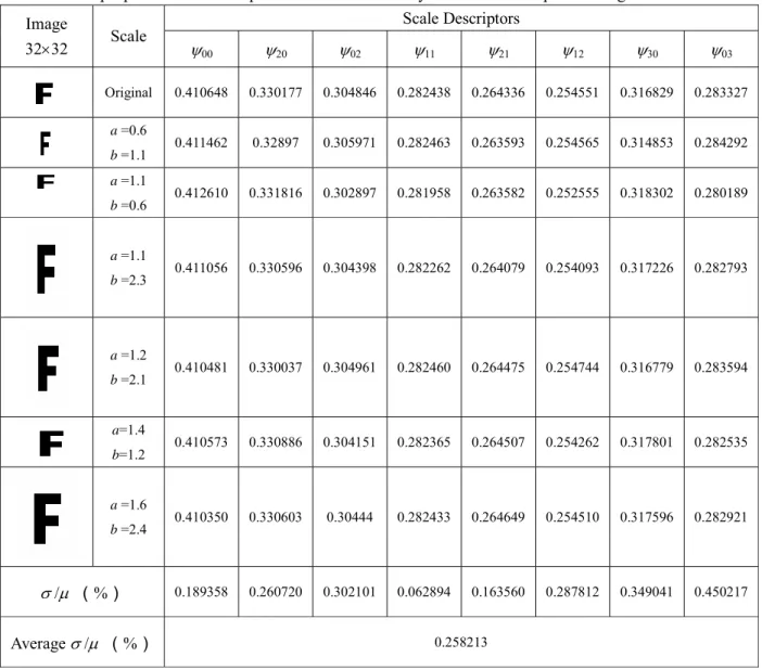
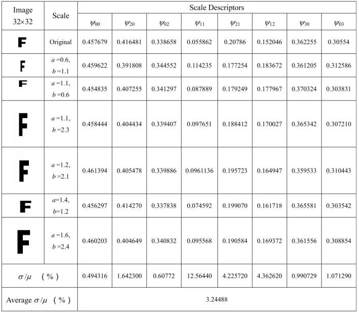
We then test the efficiency of the scale invariant descriptors. The original image shown in Table 5 is expanded or contracted with a set of scaling factors along x and y directions. The results are depicted in Table 5. Note that the coefficient γ in Eq. (49) is set to 2 in this experiment. We also compare our descriptors with the Legendre scale invariants proposed by Chong et al. [22], the results obtained with latter descriptors being shown in Table 6. From these tables, we can see that the values of the descriptors remain almost unchanged under different non-uniform scaling transformations, and that the scale invariants based on Tchebichef moments perform better than those derived from Legendre moments.

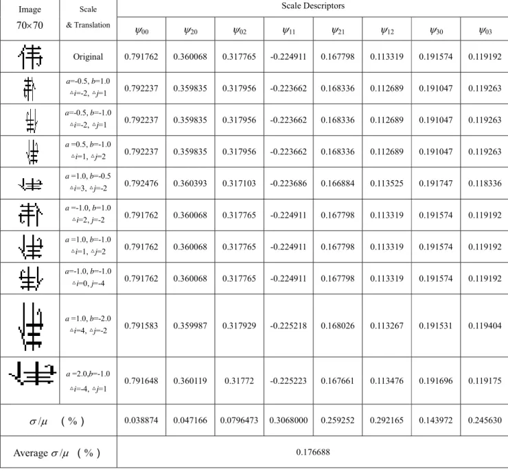
In the third experiment, we test the performance of the proposed descriptors on both translation and scale invariance. A 70×70 resolution binary Chinese character, as shown in Table 7, is arbitrary shifted from the original position, and then non-uniformly expanded, contracted or reflected. Tables 7 and 8 show respectively the computed values using the invariant descriptors proposed in this paper and those derived by Chong et al. [22] based on Legendre moments. The results again indicate the improvement brought by the present method.

We also compare the computational speed of the new approach with that of the indirect method, i.e., the method described in Subsection 2.3. A Chinese character of size 100×100 is used in this experiment. The original image is transformed with a uniform scale factor varied from 0.5 to 2 along x and y axis. The computation times required for our method and the indirect method to calculate the set of invariants of order up to 10, 20 and 30 are listed in Table 9. Note that the program was implemented in C++ on a PC Pentium IV 2.4 GHz, 256 Mb RAM. It can be seen that the new approach for deriving the moment

invariants is much faster than the method based on the geometric moment invariants.

The last experiment provides the experimental study on the classification accuracy of Tchebichef moments in both noise-free and noisy conditions. For the recognition task, we use the following feature vector ] , , , , , [Ψ₂₀ Ψ₀₂ Ψ₂₁ Ψ₁₂ Ψ₃₀ Ψ₀₃ = V (53) where Ψnm are the Tchebichef moment invariants defined in the previous Section. The objective of a

classifier is to identify the class of the unknown input character. During classification, features of the unknown character are compared against the training information being assigned to a particular class. The Euclidean distance is used as the classification measure and is defined by

∑

= − = T j tj sj k t s V v v V d 1 2 ) ( _{) ( )} , ( (54)

where Vsis the T-dimensional feature vector of unknown sample, and

) (k

t

V is the training vector of class k. In this experiment, the classification accuracy η is defined as

% 100 test in the used images of number total The images classified correctly of Number × = η (55)

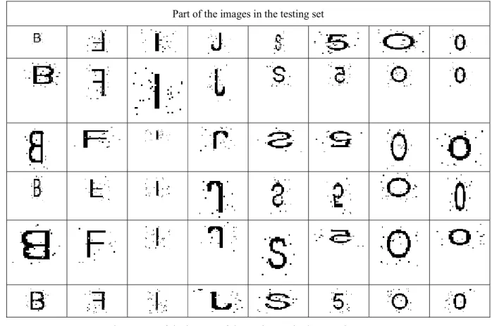
Fig. 1 shows a set of binary English characters and numbers served as the training set. The reason for choosing such a character set is that the elements in subset {B, F}, {I, J}, {S, 5}, and {O, 0} can be easily misclassified due to the similarity. The testing set is generated by scaling and translating the training set with scale factors a and b ∈ {–1.5, –1, –0.5, 0.5, 1, 1.5}, and translation Δi, Δj = –1, 0, 1 in both horizontal and vertical directions where the case of Δi = Δj = 0 is not used, forming a testing set of 2304 images. This is followed by adding salt-and pepper noise with different noise densities. Fig. 2 shows some of the testing images contaminated by 4% salt-and-pepper noise. The feature vector based on Tchebichef moment invariants are used to classify these images and its recognition accuracy is compared with that of Legendre moment invariants [22]. Table 10 shows the classification results using the full set of features. One can see from this table that 100% recognition results are obtained in noise-free case. Note that the recognition accuracy decreases with the increase of noise. However, the proposed approach performs better than the invariant descriptors based on Legendre moments in terms of the recognition accuracy for

noisy images.

The original images of the second experiment are downloaded from Website [29].The second testing set is generated in a similar way as that of the first testing set. The classification results of the image with translation and scaling transformation are depicted in Table 11. Table 11 again indicates that the Tchebichef invariant descriptors perform better in noisy conditions.

5. Discussion and conclusion

The recently proposed discrete orthogonal moments such as Tchebichef moments and Krawtchouk moments have better image representation capability than the traditional continuous moments. Because the moment invariants are useful feature descriptors for pattern recognition, we have investigated in this paper the invariance problem of Tchebichef moments. A new method to derive the translation and scale invariants of discrete Tchebichef moments was proposed. The derivation of these invariant descriptors is directly based on the Tchebichef polynomials, so that the image normalization process can be avoided. We have compared the Tchebichef moment invariants with Legendre moment invariants. Experimental results showed the superiority of Tchebichef moment invariants. This is probably due to the fact that the orthogonality of Legendre polynomials is affected when the image is discretized. On the other hand, the discretization may cause numerical errors in the computed moments.

We have only considered in this paper the translation and scale invariance properties of Tchebichef moments. The rotation invariance is not readily achieved because the Tchebichef moments, as well as the Legendre moments, fall into the same class of orthogonal moments defined in the Cartesian coordinate space [22].

We have also applied the proposed moment invariants to recognition tasks. The object recognition experiments show that the Tchebichef moment invariants perform better than the Legendre moment invariants in both noise-free and noisy conditions. Therefore, they should be potentially useful invariant descriptors for recognition tasks.

It is worth mentioning that the proposed method can be easily extended to derive the translation and scale invariants of other type of discrete orthogonal moments such as Krawtchouk moments.

Acknowledgement: This work was supported by National Basic Research Program of China under grant No. 2003CB716102 and Program for New Century Excellent Talents in University under grant No. NCET-04-0477. It has been carried out in the frame of the CRIBs, a joint international laboratory associating Southeast University, the University of Rennes 1 and INSERM, with a grant provided by the French Consulate in Shanghai. We thank the anonymous referees for their careful review and valuable comments to improve the quality of the paper.

Appendix A

Proof of Theorem 1. Using Eq. (5) and the following formula [28]

_{l k l} k l k a x l k a x ₋ = > < > < ⎟⎟ ⎠ ⎞ ⎜⎜ ⎝ ⎛ = > + <

∑

0 (A.1) we have

∑∑

∑ ∑

∑

= = − − = = = > < > < ⎟⎟ ⎠ ⎞ ⎜⎜ ⎝ ⎛ − = > < > < ⎟⎟ ⎠ ⎞ ⎜⎜ ⎝ ⎛ = > + < = + n k n k l k k l l n l k l n k k l k n n k k k n n B a x k l l x a l k B a x B a x t 0 , 0 0 , 0 , ) ( (A.2) The coefficient of < x >n–k on the right-hand side of Eq. (A2) is given by

_{k l} k l l n n a B l k l n − = − > < ⎟⎟ ⎠ ⎞ ⎜⎜ ⎝ ⎛ − −

∑

0 , (A.3)

On the other hand, substitution of Eq. (5) into Eq.(23) yields

∑

∑

∑∑

= = = − = − − < > = < > = + n k n k l k l n k l n k l k n l l k n k n n n x a a B x B a x t 0 , , 0 0 , , ( ) ( ) ) (

ν

ν

(A.4)

The coefficient of < x >n–k on the right-hand side of Eq. (A.4) is given by

∑

= − − − k i i n n k n i n v a B 0 , , ( ) (A.5)

By equating Eq. (A.3) and Eq. (A.5), we obtain

∑

∑

− = − − − − = − − − − ⎟⎟ < > − ⎠ ⎞ ⎜⎜ ⎝ ⎛ − − = 1 0 , , 0 , , , ( ) ( ) k i i n n k n i n l k k l l n n k n n k n k n B a B v a l k l n a v B (A.6)

Using the change of variable l =k−l′in the first term of the right-hand side of Eq. (A.6), we can easily

deduce Eq. (24). 

Proof of Theorem 2. Substitution of Eqs. (29) (6) into Eq. (24), we have

⎭ ⎬ ⎫ > < > − − < − − − − − > < > − < ⎩ ⎨ ⎧ + − − + − − − = > <

∑

∑

∑

∑

− = − − = − − = − = − 1 0 1 0 0 1 0 ) , ( )! ( )! 2 ( )! ( 1 )! ( )! ( ! )! 2 ( )! 2 2 ( )! ( ) , ( m j j m j k m m k l l k k l k i i k i a m n f N m n m k m k n k n a N n l k n l k l l k n k n k n a k n f (A.7)

The coefficient of < a >k–i on the right-hand side of the above equation is ⎭ ⎬ ⎫ > − − < − − − − − ⎩ ⎨ ⎧ > − < − − − − −

∑

− − = − + − 1 ) , ( )! ( )! 2 ( )! ( 1 )! ( )! ( ! )! 2 ( )! 2 2 ( )! ( k i k m k m i m k i m n f N m n m k m k n k n N n i n i k i i n k n k n (A.8)

Using the change of variable m=m′+k−iin the last term of the above equation, we can easily deduce

Eq. (30). 

REFERENCES

[1]M. K. Hu, Visual pattern recognition by moment invariants, IRE Trans. Inform. Theory, IT-8 (1962) 179-187.

[2] J. Liu, T. X. Zhang, Fast algorithm for generation of moment invariants, Pattern Recognition, 37 (2004) 1745-1756.

[3] Y. Zhu, L. C. De Silva, C. C. Ko, Using moment invariants and HMM in facial expression, Pattern Recognition Letters, 23 (2002) 83-91.

[4] C. Y. Lin, M. Wu, J. A. Bloom, I. J. Cox, M. L. Miller, Y. M. Lui, Rotation, scale, and translation resilient watermaking for images, IEEE Trans. Image Processing, 10 (2001) 767-782.

[5] C. Gope, N. Kehtarnavaz, G. Hillman, B. Wursig, An affine invariant curve matching method for photo-identification of marine mammals, Pattern Recognition, 38 (2005) 125-132.

[6] S. Sheynin, A. Tuzikov, Moment computation for objects with spline curve boundary, IEEE Trans Pattern Anal. Machine Intell., 25 (2003) 1317-1322.

[7] L. M. Luo, C. Hamitouche, J. L. Dilleseger, J. L. Coatrieux, A moment-based three-dimensional edge operator, IEEE. Trans. Biomed. Eng., 40 (1993) 693-703.

[8] C. Kan, M. D. Srinath, Combined features of cubic B-spline wavelet moments and Zernike moments for invariant character recognition, In: Proceedings of International Conference on Information Technology, (2001) 511-515.

[9] C. -H Teh, R. T. Chin, On image analysis by the method of moments, IEEE Trans. Pattern Anal. Machine Intell., 10, (1988) 496-513.

[10] R. Mukundan, K. R. Ramakrishnan, Moment functions in image analysis-Theory and applications, World Scientific, Singapore, 1998.

[11] M. R. Teague, Image analysis via the general theory of moments, J. Opt. Soc. Amer., 70 (1980) 920-930. [12] R. Mukundan, K. R. Ramakrishnan, Fast computation of Legendre and Zernike moments, Pattern

Recognition, 28 (1995) 1433-1442.

[13] H. Z. Shu, L. M. Luo, X. D. Bao, W. X. Yu, An efficient method for computation of Legendre moments,

Graphical Models, 62 (2000) 237-262.

[14] P. Nassery, K. Faez, Signature pattern recognition using pseudo-Zernike moments and a fuzzy logic classifier, In: Proceedings of ICIP-96, Switzerland, 2 (1996) 197-200.

[15]S. X. Liao, M. Pawlak, On image analysis by moments, IEEE Trans. Pattern Anal. Machine Intell., 18 (1996) 254-266.

[16]R. Palaniappan, P. Raveendran, S. Omatu, New invariant moments for non-uniformly scaled images, Pattern Anal. Appl., 3 (2000) 78-87.

[17] Z. J. Miao, Zernike moment-based image shape analysis and its application, Pattern Recognition Letters, 20 (2000) 169-177.

[18] J. Flusser, On the independence of rotation moment invariants, Pattern Recognition, 33 (2000) 1405-1410. [19] A. Khotanzad, Invariant image recognition by Zernike moments, IEEE Trans. Pattern Anal. Mach. Intell.,

12 (1990) 489-497.

[20] R. Palaniappan, P. Raveendran, S. Omatu, New invariant moments for non-uniformly scaled images, Pattern Anal. Appl., 3 (2000) 78-87.

[21] C. -W. Chong, P. Raveendran, R. Mukundan, Translation invariants of Zernike moments, Pattern Recognition, 36 (2003) 1765-1773.

[22] C. -W. Chong, P. Raveendran, R. Mukundan, Translation and scale invariants of Legendre moments, Pattern Recognition, 37 (2004) 119-129.

[23] C. -W. Chong, P. Raveendran, R. Mukundan, The scale invariants of pseudo-Zernike moments, Pattern Anal Appl., 6 (2003) 176-184.

[24] R. Mukundan, S. H. Ong, P. A. Lee, Image analysis by Tchebichef moments, IEEE Trans. Image Processing, 10 (2001) 1357-1364.

[25] P. T. Yap, R. Paramesran, S. H. Ong, Image Analysis by Krawtchouk Moments, IEEE Trans. Image Processing, 12 (2003) 1367-1377.

[26]R. Mukundan, A new class of rotational invariants using discrete orthogonal moments, In: Proceedings of the 6th IASTED Int. Conf. Signal and Image Processing, 2004, 80-84.

[27] R. Mukundan, Some computational aspects of discrete orthonormal moments, IEEE Trans. Image

Processing, 13 (2004) 1055-1059.

[28]L. Comtet, Advanced combinatorics: The Art of Finite and Infinite Expansions, D. Reidel Publishing Company, Dordrecht, Holland, 1974.

[29] http://www.mapsofworld.com/world-major-island.htm

Table 1. Selected orders of Tchebichef central moments for a Chinese character. Image Translation T ′₂₀ T ′₀₂ T ′₁₁ T ′₂₁ T ′₁₂ T ′30 T ′03 ∆i=-1 ∆j=-1 15.8669 14.1558 17.7847 -27.2982 -24.3173 -32.1257 -21.8373 ∆i=-1 ∆j=+1 15.8669 14.1558 17.7847 -27.2982 -24.3173 -32.1257 -21.8373 ∆i=+1 ∆j=-1 15.8669 14.1558 17.7847 -27.2982 -24.3173 -32.1257 -21.8373 32×32 ∆i=+1 ∆j=+1 15.8669 14.1558 17.7847 -27.2982 -24.3173 -32.1257 -21.8373

μ

σ

/ （%） 0.0000 0.0000 0.0000 0.0000 0.0000 0.0000 0.0000

Table 2. Selected orders of Tchebichef central moments for an English letter.

Image Translation T ′20 T ′02 T ′11 T ′21 T ′12 T ′30 T ′03 ∆i=-2 ∆j=-1 4.50151 4.53576 5.95335 -7.74391 -7.83157 -5.94542 -6.17103 ∆i=-1 ∆j=+3 4.50151 4.53576 5.95335 -7.74391 -7.83157 -5.94542 -6.17103 ∆i=+2 ∆j=-3 4.50151 4.53576 5.95335 -7.74391 -7.83157 -5.94542 -6.17103 32×32 ∆i=+1 ∆j=+4 4.50151 4.53576 5.95335 -7.74391 -7.83157 -5.94542 -6.17103 σ /μ （%） 0.0000 0.0000 0.0000 0.0000 0.0000 0.0000 0.0000

Table 3. Selected orders of Tchebichef central moments for an English letter being symmetric along x-axis.

Table 4. Selected orders of Legendre moments for an English letter being symmetric along x-axis. Image Translation T ′₂₀ T ′₀₂ T ′₁₁ T ′21 T ′12 T ′30 T ′03 ∆i=-1 ∆j=-1 4.63676 4.87909 6.16477 -7.78394 -8.16659 -5.82650 -7.24762 ∆i=-1 ∆j=+1 4.63676 4.87909 6.16477 -7.78394 -8.16659 -5.82650 -7.24762 ∆i=+1 ∆j=-1 4.63676 4.87909 6.16477 -7.78394 -8.16659 -5.82650 -7.24762 32×32 ∆i=+1 ∆j=+1 4.63676 4.87909 6.16477 -7.78394 -8.16659 -5.82650 -7.24762 σ/μ （%） 0.0000 0.0000 0.0000 0.0000 0.0000 0.0000 0.0000 Image Translation L′20 L′02 L′11 L′21 L′12 L′30 L′03 ∆i=-1 ∆j=-1 -0.157269 -0.139269 0.00000 0.00000 0.0032065 0.0023617 0.00000 ∆i=-1 ∆j=+1 -0.157269 -0.139269 0.00000 0.00000 0.0032065 0.0023617 0.00000 ∆i=+1 ∆j=-1 -0.157269 -0.139269 0.00000 0.00000 0.0032065 0.0023617 0.00000 32×32 ∆i=+1 ∆j=+1 -0.157269 -0.139269 0.00000 0.00000 0.0032065 0.0023617 0.00000 σ/μ （%） 0.0000 0.0000 0.0000 0.0000 0.0000 0.0000 0.0000

Table 5. The proposed scale descriptors for a non-uniformly contracted or expanded English letter Scale Descriptors Image 32×32 Scale ψ00 ψ20 ψ02 ψ11 ψ21 ψ12 ψ30 ψ03 Original 0.410648 0.330177 0.304846 0.282438 0.264336 0.254551 0.316829 0.283327 a =0.6 b =1.1 0.411462 0.32897 0.305971 0.282463 0.263593 0.254565 0.314853 0.284292 a =1.1 b =0.6 0.412610 0.331816 0.302897 0.281958 0.263582 0.252555 0.318302 0.280189 a =1.1 b =2.3 0.411056 0.330596 0.304398 0.282262 0.264079 0.254093 0.317226 0.282793 a =1.2 b =2.1 0.410481 0.330037 0.304961 0.282460 0.264475 0.254744 0.316779 0.283594 a=1.4 b=1.2 0.410573 0.330886 0.304151 0.282365 0.264507 0.254262 0.317801 0.282535 a =1.6 b =2.4 0.410350 0.330603 0.30444 0.282433 0.264649 0.254510 0.317596 0.282921 σ /μ （%） 0.189358 0.260720 0.302101 0.062894 0.163560 0.287812 0.349041 0.450217 Average σ /μ （%） 0.258213

Table 6 The scale invariant descriptors of Legendre moments for a non-uniformly contracted or expanded English letter Scale Descriptors Image 32×32 Scale ψ00 ψ20 ψ02 ψ11 ψ21 ψ12 ψ30 ψ03 Original 0.457679 0.416481 0.338658 0.055862 0.20786 0.152046 0.362255 0.30554 a =0.6, b =1.1 0.459622 0.391808 0.344552 0.114235 0.177254 0.183672 0.361205 0.312586 a =1.1, b =0.6 0.454835 0.407255 0.341297 0.087889 0.179249 0.177967 0.370324 0.303831 a =1.1, b =2.3 0.458444 0.404434 0.339407 0.097651 0.188412 0.170027 0.365342 0.307210 a =1.2, b =2.1 0.461394 0.405478 0.339886 0.0961136 0.195723 0.164947 0.359533 0.310443 a=1.4, b=1.2 0.456297 0.414270 0.337838 0.074592 0.199070 0.161718 0.365581 0.303542 a =1.6, b =2.4 0.460203 0.404649 0.340832 0.095568 0.190584 0.169372 0.361556 0.308854 σ /μ （%） 0.494316 1.642300 0.60772 12.56440 4.225720 4.362620 0.990729 1.071290 Average σ /μ （%） 3.24488

Table 7. The proposed translation and scale invariant descriptors for a translated, non-uniformly contracted, expanded and reflected Chinese character

Scale Descriptors Image 70×70 Scale & Translation _ψ 00 ψ20 ψ02 ψ11 ψ21 ψ12 ψ30 ψ03 Original 0.791762 0.360068 0.317765 -0.224911 0.167798 0.113319 0.191574 0.119192 a=-0.5, b=1.0 △i=-2, △j=1 0.792237 0.359835 0.317956 -0.223662 0.168336 0.112689 0.191047 0.119263 a=-0.5, b=-1.0 △i=-2, △j=1 0.792237 0.359835 0.317956 -0.223662 0.168336 0.112689 0.191047 0.119263 a =0.5, b=-1.0 △i=1, △j=2 0.792237 0.359835 0.317956 -0.223662 0.168336 0.112689 0.191047 0.119263 a =1.0, b=-0.5 △i=3, △j=-2 0.792476 0.360393 0.317103 -0.223686 0.166884 0.113525 0.191747 0.118336 a =-1.0, b=1.0 △i=2, j=-2 0.791762 0.360068 0.317765 -0.224911 0.167798 0.113319 0.191574 0.119192 a =1.0, b=-1.0 △i=1, △j=2 0.791762 0.360068 0.317765 -0.224911 0.167798 0.113319 0.191574 0.119192 a=-1.0, b=-1.0 △i=0, j=-4 0.791762 0.360068 0.317765 -0.224911 0.167798 0.113319 0.191574 0.119192 a =1.0, b=-2.0 △i=4, △j=-2 0.791583 0.359987 0.317929 -0.225218 0.168026 0.113267 0.191531 0.119404 a =2.0,b=-1.0 △i=-4, △j=1 0.791648 0.360119 0.31772 -0.225223 0.167661 0.113476 0.191696 0.119175 σ /μ （%） 0.038874 0.047166 0.0796473 0.3068000 0.259252 0.292165 0.143972 0.245630 Average σ /μ （%） 0.176688

Table 8 The translation and scale invariant descriptors of Legendre moments for a shifted, non-uniformly contracted, expanded and reflected Chinese character

Scale Descriptors Image 70×70 Scale &Translation ψ₀₀ ψ₂₀ ψ₀₂ ψ₁₁ ψ₂₁ ψ₁₂ ψ₃₀ ψ₀₃ Original 0.572661 0.434886 0.383836 -0.349139 0.296913 0.200528 0.248021 0.154343 a=-0.5, b=1.0 △i=-2, △j=1 0.571835 0.436255 0.383283 -0.347298 0.298995 0.19947 0.249449 0.15412 a=-0.5, b=-1.0 △i=-2, △j=1 0.571835 0.436255 0.383283 -0.347298 0.298995 0.19947 0.249449 0.15412 a =0.5, b=-1.0 △i=1, △j=2 0.571835 0.436255 0.383283 -0.347298 0.298995 0.19947 0.249449 0.15412 a =1.0, b=-0.5 △i=3, △j=-2 0.572653 0.43488 0.385055 -0.347774 0.295752 0.201951 0.248018 0.154812 a =-1.0, b=1.0 △i=2, j=-2 0.572661 0.434886 0.383836 -0.349139 0.296913 0.200528 0.248021 0.154343 a =1.0, b=-1.0 △i=1, △j=2 0.572661 0.434886 0.383836 -0.349139 0.296913 0.200528 0.248021 0.154343 a=-1.0, b=-1.0 △i=0, j=-4 0.572661 0.434886 0.383836 -0.349139 0.296913 0.200528 0.248021 0.154343 a =1.0, b=-2.0 △i=4, △j=-2 0.572662 0.434886 0.383533 -0.349479 0.297202 0.200174 0.248021 0.154226 a =2.0,b=-1.0 △i=-4, △j=1 0.572863 0.434545 0.383972 -0.349597 0.296396 0.200791 0.247668 0.154397 σ /μ （%） 0.0715249 0.156332 0.136584 0.274517 0.389516 0.379464 0.285477 0.132819 Average σ /μ （%） 0.247729625

Table 9. The comparison of CPU elapsed time (ms) for the proposed and indirect methods

100×100 Scale

Factor

Orders of

Descriptor Proposed Method Indirect Method

0~10 50 280 0~20 230 1412 0.5 0~30 891 5738 0~10 160 912 0~20 551 3364 1.0 0~30 1522 9904 0~10 321 2033 0~20 1082 6730 1.5 0~30 2624 16865 0~10 571 3495 0~20 1823 11457 2.0 0~30 4086 26428 Table 10

Classification results of the image with translation and scale transformation Salt-and-pepper Noise Noise-free 1% 2% 3% 4% Legendre 100% 84.24% 76.14% 71.8% 66.5% Tchebichef 100% 89.53% 83.28% 80.5% 75.7% Table 11

Classification results of the image with translation and scale transformation Salt-and-pepper Noise Noise-free 1% 2% 3% 4% Legendre 100% 85.45% 77.42% 72.36% 68.50% Tchebichef 100% 91.84% 83.75% 81.60% 78.23%

Fig. 1. Binary images as training set for invariant character recognition in the experiment

Part of the images in the testing set

Fig. 2. Part of the images of the testing set in the experiment

(a) (b) (c) (d) (e)

Fig. 3. Set of test images (100×100). (a) Image of island of Cozume. (b) Image of Finland. (c) Image of island of Grand. (d) Image of island of Greenland. (e) Image of island of Iceland.

About the Author—HONGQING ZHU obtained her Ph. D. degree in 2000 from Shanghai Jiao Tong University. From 2003 to 2005, she was a postdoctoral fellow in Department of Biology and Medical Engineering of Southeast University. Now, she is an associate professor in East China University of Science & Technology. Her current research is mainly focused on image reconstruction, image segmentation, image compression, and pattern recognition.

About the Author—HUAZHONG SHU received the B. S. Degree in Applied Mathematics from Wuhan University, China, in 1987, and a Ph. D. degree in Numerical Analysis from the University of Rennes (France) in 1992. He was a postdoctoral fellow with the Department of Biology and Medical Engineering, Southeast University, from 1995 to 1997. He is now with the Department of Computer Science and Engineering of the same university. His recent work concentrates on the image analysis, pattern recognition and fast algorithms of digital signal processing. Dr. SHU is a member of IEEE.

About the Author—TING XIA was born in 1980. She received the B.S degree and Ms. Degree in Biomedical Engineering in 2003 and 2006 from Southeast University, respectively. Her research interest is mainly focused on pattern recognition and image processing.

About the Author—LIMIN LUO obtained his Ph. D. degree in 1986 from the University of Rennes (France). Now he is a professor of the Department of Computer Science and Enginnering, Southeast University, Nanjing, China. He is the author and co-author of more than 80 papers. His current research interests include medical imaging, image analysis, computer-assisted systems for diagnosis and therapy in medicine, and computer vision. Dr LUO is a senior member of the IEEE. He is an associate editor of IEEE Eng. Med. Biol. Magazine and Innovation et Technologie

en Biologie et Medecine (ITBM).

About the Author—JEAN LOUIS COATRIEUX received the PhD and State Doctorate in Sciences in 1973 and 1983, respectively, from the University of Rennes 1, Rennes, France. Since 1986, he has been Director of Research at the National Institute for Health and Medical Research (INSERM), France, and since 1993 has been Professor at the New Jersey Institute of Technology, USA. He is also Professor at Telecom Bretagne, Brest, France. He has been the Head of the Laboratoire Traitement du Signal et de l'Image, INSERM, up to 2003. His experience is related to 3D images, signal processing, pattern recognition, computational modeling and complex systems with applications in integrative biomedicine. He published more than 300 papers in journals and conferences and edited many books in these areas. He has served as the Editor-in-Chief of the IEEE Transactions on Biomedical Engineering (1996-2000) and is in the Boards of several journals. Dr. COATRIEUX is a fellow member of IEEE. He has received several awards from IEEE (among which the EMBS Service Award, 1999 and the Third Millennium Award, 2000) and he is Doctor Honoris Causa from the Southeast University, China.