HAL Id: hal-01214695
https://hal.archives-ouvertes.fr/hal-01214695v3
Submitted on 5 Sep 2016
HAL is a multi-disciplinary open access
archive for the deposit and dissemination of
sci-entific research documents, whether they are
pub-lished or not. The documents may come from
teaching and research institutions in France or
abroad, or from public or private research centers.
L’archive ouverte pluridisciplinaire HAL, est
destinée au dépôt et à la diffusion de documents
scientifiques de niveau recherche, publiés ou non,
émanant des établissements d’enseignement et de
recherche français ou étrangers, des laboratoires
publics ou privés.
Microtexture Inpainting through Gaussian Conditional
Simulation
Bruno Galerne, Arthur Leclaire, Lionel Moisan
To cite this version:
Bruno Galerne, Arthur Leclaire, Lionel Moisan. Microtexture Inpainting through Gaussian
Condi-tional Simulation. IEEE InternaCondi-tional Conference on Acoustics, Speech, and Signal Processing, Mar
2016, Shanghai, China. �10.1109/ICASSP.2016.7471867�. �hal-01214695v3�
MICROTEXTURE INPAINTING THROUGH GAUSSIAN CONDITIONAL SIMULATION
Bruno Galerne
?, Arthur Leclaire
†, Lionel Moisan
? ∗?
Universit´e Paris Descartes, MAP5, CNRS UMR 8145, France.
†
CMLA, ENS Cachan, CNRS, Universit´e Paris-Saclay, 94235 Cachan, France
ABSTRACT
Image inpainting consists in filling missing regions of an im-age by inferring from the surrounding content. In the case of texture images, inpainting can be formulated in terms of conditional simulation of a stochastic texture model. Many texture synthesis methods thus have been adapted to texture inpainting, but these methods do not offer theoretical guaran-tees since the conditional sampling is in general only approx-imate. Here we show that in the case of Gaussian textures, inpainting can be addressed with perfect conditional simula-tion relying on kriging estimasimula-tion. We thus obtain a micro-texture inpainting algorithm that is able to fill holes of any shape and size in an efficient manner while respecting exactly a stochastic model.
Index Terms— Inpainting, Gaussian texture, texture syn-thesis, conditional simulation, kriging
1. INTRODUCTION
Since the seminal papers [1, 2, 3], random phase fields have proven to be a powerful tool for microtexture modeling. In particular, given a microtexture, a Gaussian model can be eas-ily derived and sampled [4] and latter approximated by a spot noise model to allow for fast by-example synthesis [5]. In addition, the theoretical benefits of the Gaussian model have been exploited to address texture analysis [6] and texture mix-ing [7]. In this paper, we take advantage of the Gaussian model in order to address microtexture inpainting.
The inpainting problem consists in recovering hidden parts of an image based on the surrounding content. Many methods have been proposed for inpainting, falling into three categories. The first are deterministic methods which use a variational or PDE-based framework to fill the miss-ing regions by connectmiss-ing the edges or level lines in a way that respects the Gestaltist’s good continuation prin-ciple [8, 9, 10, 11, 12, 13, 14, 15]. The common drawback of these methods is their inability to handle texture precisely.
The second are stochastic methods. Inpainting is by essence an ill-posed problem. However, if one has a perti-nent stochastic model p(u) for the whole image u, a perfect
∗This work has been partially funded by the French Research Agency (ANR) under grant nr ANR-14-CE27-001 (MIRIAM)
inpainting solution can be obtained by conditional simula-tion, that is simulating an image u with distribution p(u) given the known values of u. This stochastic point of view is not really helpful in general since one cannot sample the distribution of realistic images. However, this approach is of particular interest when dealing with texture images since they are often well represented by tractable stochastic models. The first works in the direction of stochastic in-painting suggest to fill the masked zone by matching specific statistics, like co-occurrence matrices [16] or histograms of filter responses [17]. Truly conditional methods later ap-peared based on Markov random fields, which are inherently adapted to conditional sampling [18]. Using patch compar-ison to approximate local conditional sampling, the authors of [19, 20] were led to a celebrated non-parametric texture synthesis algorithm which can also be used for hole filling. However, these synthesis algorithms may degenerate after a spatial boundary (growing garbage effect), and besides are quite dependent on the filling order, thus not ensuring the prolongation of large-scale features.
Taking profit of the first attempts in deterministic and stochastic inpainting, hybrid methods have emerged, which consist in filling both geometric and textural contents in a coherent manner. After the proposition of [21] to extend non-parametric sampling to general image synthesis, several authors improved this work by varying the pixel filling or-der [22, 23, 24]. Other methods suggest to separate geometry and texture and to inpaint them either with two different tech-niques [25] or to minimize a unified functional [26]. The last work paves the way for inpainting with adapted dic-tionaries [27, 28, 29, 30]. More recently, several authors gave a unified view of example-based image inpainting in a variational framework [31, 32].
These methods are able to produce a satisfying result on a large class of images with a reasonable computational time, but in general do not provide any theoretical guarantee in the synthesized content. In contrast, we demonstrate in this paper that if one restricts to a Gaussian random model, mi-crotexture inpainting can be achieved by perfect conditional sampling. Our algorithm relies on kriging estimation [33] and fills holes with two independent components, namely the kriging component which extends long scale structures from the hole boundary, and the innovation component which adds
an independently generated textural content containing small scale details. The proposed algorithm can inpaint holes of any shape and size, provided that a faithful Gaussian texture model can be estimated within the unmasked image area. For large holes, this algorithm does not suffer from the growing garbageeffect encountered in [19], and besides, edge-like structures in the textures are naturally restored in a way that respects the covariance.
Texture inpainting was addressed in [34, 35] with krig-ing estimation, but this does not amount to samplkrig-ing a global Gaussian model since the innovation component is missing (see Section 4). Also, texture synthesis was addressed in [36] by progressive filling with Gaussian conditional patch mod-els, but in this case too the global model is not Gaussian.
2. GAUSSIAN CONDITIONAL SIMULATION In this section, following [33], we rely on kriging estimation to explain the perfect conditional sampling of Gaussian ran-dom vectors that is at the heart of our microtexture inpainting algorithm.
Let Ω be a finite set. For a set A ⊂ Ω and a function f : Ω → R we denote by |A| the cardinality of the finite set A, and f|Athe restriction to A of the function f . Let (F (x))x∈Ω
be a Gaussian vector with mean zero (for the sake of simplic-ity) and covariance function Γ(x, y) = Cov(F (x), F (y)) = E(F (x)F (y)), x, y ∈ Ω.
Given prescribed values ϕ : C → R on a set C ⊂ Ω of con-ditioning points, conditional Gaussian simulation consists in sampling the conditional distribution of F given that F|C= ϕ.
One defines the kriging estimator at x ∈ Ω as the condi-tional expectation F∗(x) = E( F (x) | F (c) , c ∈ C ). This means that F∗(x) is the best least-square estimation of F (x) that can be obtained as a measurable function of (F (c))c∈C.
In particular for all x ∈ C, F∗(x) = F (x). A standard result of probability theory [37] ensures that in the Gaussian case F∗(x) is the orthogonal projection of F (x) on the subspace of linear combinations of (F (c))c∈C(for the L2-distance
be-tween square-integrable random variables). Hence, there exist coefficients (λc(x))c∈Csuch that
F∗(x) =X
c∈C
λc(x)F (c). (1)
These deterministic numbers (λc(x))c∈Care called the
krig-ing coefficients. The followkrig-ing theorem is the core result for conditional Gaussian simulation.
Theorem 2.1 ([33]). F∗andF − F∗are independent. Con-sequently, ifG is independent of F and has the same distri-bution, thenH = F∗+ (G − G∗) has the same distribution asF and satisfies H|C= F|C.
Proof. Due to the orthogonal projection, (F∗, F − F∗) is a
Gaussian vector whose components F∗ and F − F∗ are un-correlated and thus independent.
A conditional sample of F given F|C = ϕ can thus be
obtained with ϕ∗ + G − G∗ where the kriging compo-nent ϕ∗ is defined by ϕ∗(x) =P
c∈Cλc(x)ϕ(c), x ∈ Ω
and where the independent component G − G∗ is called the innovation component. To do so one needs to com-pute the kriging coefficients (λc(x))c∈C introduced in (1).
Since F∗(x) − F (x) is orthogonal to F (c), we obtain that E(F∗(x)F (c)) = E(F (x)F (c)) = Γ(x, c), and using (1) to substitute F∗(x) shows that (λc(x))c∈C is a solution of the
following |C| × |C| linear system ∀c ∈ C, X
d∈C
λd(x)Γ(d, c) = Γ(x, c). (2)
In the following, we will assume that the matrix Γ|C×C is
invertible (which turned out to be true in all our inpainting experiments) so that this system admits a unique solution. If we denote by Λ = (λc(x))x∈Ω, c∈C the |Ω| × |C|
ma-trix of all kriging coefficients, the previous system rewrites Λ = Γ|Ω×CΓ−1|C×C, where Γ|Ω×C and Γ|C×C are the
restric-tions of the covariance matrix Γ. Finally, writing the Gaus-sian vectors in column, sampling F given F|C = ϕ amounts
to sampling
Λϕ + G − ΛG|C, where Λ = Γ|Ω×CΓ−1|C×C (3)
where G has the same distribution as F and is independent of F . The required number of operations is O(|C|3+ |Ω||C|)
in addition to the simulation cost for G.
3. MICROTEXTURE INPAINTING
In this section, we use the Gaussian conditional sampling scheme described in the previous section to perform micro-texture inpainting. The input is a masked micro-texture u : Ω → R the values of which are unknown on the mask domain M ⊂ Ω, and we want to sample these values based on the unmasked values in Mc. This amounts to adopting a Gaus-sian texture model U on Ω, and to sample it on M given the surrounding values. This raises two main difficulties: 1) One must estimate the Gaussian model for U from the masked image u; 2) The computation of the kriging components must be practical, without a cubic complexity in |Mc|3.
3.1. Gaussian Texture Model Estimation
The Gaussian model that we use for conditional simula-tion is given by an asymptotic discrete spot noise (ADSN), which is the convolution of a finitely-supported function h : Z2 → R with a normalized Gaussian white noise on the discrete plane Z2. This ADSN has zero mean and covariance Γ(x, y) = (h ∗ ˜h)(x − y), x, y ∈ Z2, where ˜h(x) = h(−x).
Note that Γ(x, y) only depends on x − y since the ADSN is stationary. In order to estimate an ADSN from the masked exemplar, we consider a subimage v of u defined on a subdo-main ω ⊂ Mc. Following [4, 5], we compute the empirical
mean ¯v and the normalized spot tv = √1
Original Masked input Conditioning set Kriging component Innovation component Inpainted result Fig. 1. Inpainting with the oracle Gaussian model. The masked texture is inpainted with a Gaussian model estimated on the non masked input using a conditioning set of 3-pixel-width along the mask boundary. The kriging component and the innovation component are displayed. As one can see on the result, the conditional inpainting is able to fill both small and large holes, whatever the regularity of the boundary.
extend by zero-padding to Z2. The ADSN is then simply given by the convolution tv∗ W where W is a normalized
Gaussian white noise on Z2. We must choose ω large enough
to capture a representative piece of the desired texture. 3.2. Textural Inpainting Algorithm
Ideally one would consider the conditioning set C = Mc, but because of the O(|C|3) complexity, we restrict C to a band of width w pixels along the outside boundary of M (Let us men-tion that in the case where U has a Markov property with a neighborhood of width w, this restriction of the conditioning set would still give a perfect conditional sampling given all the values in Mc). We then sample U on M given U
|C = u|C
with the algorithm explained in Section 2. However, we ex-ploit the stationarity of our Gaussian model to compute effi-ciently the kriging component. Indeed, thanks to stationarity, a matrix-vector multiplication with the covariance matrix Γ is a convolution by the image cv = tv∗ ˜tv. Hence to compute
the kriging component ϕ∗= Λϕ = Γ|Ω×C(Γ−1|C×Cϕ) we first
compute ψ = Γ−1|C×Cϕ that we extend by zero-padding to get a function Ψ on Ω, and then compute ϕ∗= cv∗ Ψ. The whole
process is summarized in Algorithm 1.
Algorithm 1: Microtexture inpainting Inputs: Mask M ⊂ Ω, values of the texture u on Mc - From a restriction v of u to a subdomain ω ⊂ Mc, compute the mean ¯v, tv= √1
|ω|(v − ¯v) ∈ R Ω
(extended by 0 outside ω), and cv = tv∗ ˜tv
- Store the matrix Γ|C×C(c, d) = cv(c − d), c, d ∈ C
- Draw an ADSN sample U = tv∗ W
- Compute ψ1= Γ−1|C×C(u|C− ¯v) and ψ2= Γ−1|C×CU|C
- Extend ψ1and ψ2by zero-padding to get Ψ1and Ψ2
- Compute the kriging components (u − ¯v)∗= cv∗ Ψ1
and U∗= cv∗ Ψ2
Output: ¯v + (u − ¯v)∗+ U − U∗
Concerning the complexity, Γ−1|C×Cϕ is computed with standard numerical techniques in O(|C|3). Then, the kriging components is obtained with the discrete Fourier transform in O(|Ω| log |Ω|), which is the complexity to generate the ADSN sample U . Thus, the number of conditioning points must stay low for the conditional simulation to be feasible.
Extension to Color Images Algorithm 1 can be straight-forwardly adapted to color textures. Indeed, the simulation of the color ADSN model is identical to the grayscale case, provided that we convolve the three channels by the same Gaussian white noise [4]. Besides, the kriging framework can be adapted by taking the conditional expectation with re-spect to the three channels of conditional values. In the end, it amounts to computing a larger matrix Γ containing all the cross-correlations between the three channels. Then, the ma-trix Γ−1|C×C is of size 3|C| × 3|C|, and the convolution involved in ΓΩ×Cis now a convolution by a matrix-valued function.
4. RESULTS
First, in Fig. 1 we validate the methodology based on condi-tional simulation by inpainting a masked texture with a pre-viously estimated Gaussian model. One can see that, in con-trast to PDE-based methods, this algorithm is able to fill holes in textures of any size and shape. In particular, the kriging component extends edge-like structures and the innovation component adds local details, while globally preserving the texture covariance. This reveals the crucial difference with methods solely using the kriging component [34, 35].
Let us also discuss on this example the influence of the parameter w which is the width of the conditioning points. Intuitively, this value must not be too small in order to get a sufficient summary of the surrounding context based on the conditioning set C, but also not too large to keep a reasonable computational time (see Subsection 3.2). In our experiments we chose the value w = 3. We observed in other experi-ments (not shown here) that this is the minimal value ensur-ing a good line preservation. As already said, with a Gaussian Markov model, restricting the conditioning points to the mask border would not affect the conditional distributions. Let us mention however that the ADSN models that we use here do not satisfy the Markov property. But the visual impact of this conditioning restriction seems visually harmless.
Now, let us present microtexture inpainting with a Gaus-sian model estimated on the masked exemplar. In Fig. 2, we inpaint a circular hole in the left part of the texture while learning the Gaussian model on the right part. One can ob-serve that the algorithm produces a satisfying result on the two first examples because the hole cannot be perceived in the inpainted texture and it may be difficult to distinguish the
Fig. 2. Examples of microtexture inpainting. Here, a Gaussian texture model was estimated on the masked exemplar (middle col-umn) in the red rectangle, and conditionally sampled to get the in-painted texture (right column). The inpainting is satisfactory because the output has similar aspect than the original unmasked texture (left column) while being different on the mask.
original and the output. The result is however slightly less sat-isfying on the third example because the corresponding Gaus-sian model exhibits interference patterns which are not visible in the original.
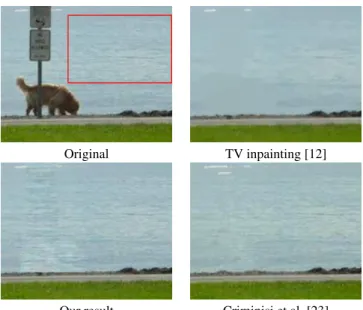
In Fig. 3, we compare our method to the one of [12] based on the total variation (TV), and to the example-based method of [23]. As expected, textures are completely lost with the TV-based model. In contrast, the result of [23] is more pre-cise, but the border of the inpainted domain is still visible. It is also the case with our method, which produces a more textured pattern.
Our Gaussian inpainting algorithm is also compared to Efros-Leung algorithm in Fig. 4. As one can see, the fre-quency content of the estimated Gaussian model is precisely reproduced in the filled zone. In contrast, Efros-Leung al-gorithm fails to reproduce the long-range correlations which exist in this microtexture. In Fig. 4 we also show the kriging component ¯v+(u−¯v)∗involved in the conditional simulation; one can see that this component contains long-range diagonal correlations that are characteristic of this wood texture.
To conclude, this paper shows that Gaussian conditional sampling is an interesting algorithm to fill large holes in mi-crotextures provided that the Gaussian model has been prop-erly estimated. For small to medium holes, the proposed al-gorithm is very efficient (the results of Figures 2, 3 were ob-tained in about 1 sec.). Its main limitation is that the Gaussian model is only valid for a limited class of texture. Still, extend-ing Gaussian conditional method to non-stationary Gaussian random fields could be of potential interest to inpaint non-texture images.
Original TV inpainting [12]
Our result Criminisi et al. [23] Fig. 3. Comparison with [12, 23]. On this example taken from [23], we compare our result (bottom left) to [12] (top right, obtained with the implementation available at [38]) and to [23] (bottom right). The Gaussian model that we used was estimated in the red rectangle shown on the original (top left). As one can see, the TV inpaint-ing is not able to preserve texture. In contrast, the result of [23] is comparable to ours.
Original Kriging component
Efros-Leung Our result
Fig. 4. Comparison with Efros-Leung [19]. The original image (top left) was inpainted by learning a Gaussian model in the red rect-angle. The kriging component is shown in the top right. In the sec-ond row, we show the result of [19] (left) and our result (right). As one can see, our algorithm better preserves the frequency content of the estimated texture, and the filled region naturally blends with the surrounding content.
Acknowledgments. This work has been partially funded by the French Research Agency (ANR) under grant nro ANR-14-CE27-0019 (MIRIAM).
5. REFERENCES
[1] J.P. Lewis, “Texture Synthesis for Digital Painting,” in Pro-ceedings of SIGGRAPH, 1984, pp. 245–252.
[2] J.P. Lewis, “Methods for Stochastic Spectral Synthesis,” in Proceedings on Graphics Interface, 1986, pp. 173–179. [3] J. J. Van Wijk, “Spot noise texture synthesis for data
visualiza-tion,” in Proc. of SIGGRAPH, 1991, vol. 25, pp. 309–318. [4] B. Galerne, Y. Gousseau, and J.-M. Morel, “Random Phase
Textures: Theory and Synthesis,” IEEE Transactions on Image Processing, vol. 20, no. 1, pp. 257–267, 2011.
[5] B. Galerne, A. Leclaire, and L. Moisan, “A Texton for Fast and Flexible Gaussian Texture Synthesis,” in Proceedings of EUSIPCO. 2014, pp. 1686–1690, IEEE.
[6] A. Desolneux, L. Moisan, and S. Ronsin, “A compact represen-tation of random phase and Gaussian textures,” in Proceedings of ICASSP, 2012, pp. 1381–1384.
[7] G. Xia, S. Ferradans, G. Peyr´e, and J. Aujol, “Synthesizing and Mixing Stationary Gaussian Texture Models,” SIAM Journal on Imaging Sciences, vol. 7, no. 1, pp. 476–508, 2014. [8] S. Masnou and J.-M. Morel, “Level lines based disocclusion,”
in Proceedings of ICIP, 1998, vol. 3, pp. 259–263.
[9] M. Bertalmio, G. Sapiro, V. Caselles, and C Ballester, “Image Inpainting,” in Proc. of SIGGRAPH, 2000, pp. 417–424. [10] C. Ballester, M. Bertalmio, V. Caselles, G. Sapiro, and
J. Verdera, “Filling-in by joint interpolation of vector fields and graylevels,” IEEE TIP, vol. 10, no. 8, pp. 1200–1211, 2001. [11] T.F. Chan and J. Shen, “Nontexture inpainting by
curvature-driven diffusions,” Journal of Visual Communication and Im-age Representation, vol. 12, no. 4, pp. 436–449, 2001. [12] T.F. Chan and J. Shen, “Mathematical models for local
nontex-ture inpaintings,” SIAM Journal on Applied Mathematics, vol. 62, no. 3, pp. 1019–1043, 2002.
[13] S. Esedoglu and J. Shen, “Digital inpainting based on the Mumford-Shah-Euler image model,” European Journal of Ap-plied Mathematics, vol. 13, no. 4, pp. 353–370, 2002. [14] D. Tschumperl´e, “Fast anisotropic smoothing of multi-valued
images using curvature-preserving PDE’s,” International Jour-nal of Computer Vision, vol. 68, no. 1, pp. 65–82, 2006. [15] F. Bornemann and T. M¨arz, “Fast image inpainting based on
coherence transport,” Journal of Mathematical Imaging and Vision, vol. 28, no. 3, pp. 259–278, 2007.
[16] T. Malzbender and S. Spach, “A Context Sensitive Texture Nib,” in Com. with Virtual Worlds, pp. 151–163. 1993. [17] H. Igehy and L. Pereira, “Image replacement through texture
synthesis,” in Proceedings of ICIP, 1997, vol. 3, pp. 186–189. [18] G. Winkler, Image Analysis, Random Fields and Markov Chain Monte Carlo Methods: A Mathematical Introduction, Springer, 2006.
[19] A. A. Efros and T. K. Leung, “Texture synthesis by non-parametric sampling,” in Proceedings of ICCV, 1999, vol. 2, pp. 1033–1038.
[20] L.Y. Wei and M. Levoy, “Fast texture synthesis using tree-structured vector quantization,” in Proceedings of SIGGRAPH, 2000, pp. 479–488.
[21] R. Bornard, E. Lecan, L. Laborelli, and J.H. Chenot, “Missing data correction in still images and image sequences,” in Pro-ceedings of the tenth ACM international conference on Multi-media, 2002, pp. 355–361.
[22] I. Drori, D. Cohen-Or, and H. Yeshurun, “Fragment-based im-age completion,” in ACM TOG, 2003, vol. 22, pp. 303–312. [23] A. Criminisi, P. P´erez, and K. Toyama, “Region filling and
object removal by exemplar-based image inpainting,” IEEE TIP, vol. 13, no. 9, pp. 1200–1212, 2004.
[24] F. Cao, Y. Gousseau, S. Masnou, and P. P´erez, “Geometrically guided exemplar-based inpainting,” SIAM Journal on Imaging Sciences, vol. 4, no. 4, pp. 1143–1179, 2011.
[25] M. Bertalmio, L. Vese, G. Sapiro, and S. Osher, “Simultaneous structure and texture image inpainting,” IEEE Transactions on Image Processing, vol. 12, no. 8, pp. 882–889, 2003.
[26] M. Elad, J. L. Starck, P. Querre, and D. L. Donoho, “Simulta-neous cartoon and texture image inpainting using morphologi-cal component analysis (MCA),” Applied and Computational Harmonic Analysis, vol. 19, no. 3, pp. 340–358, 2005. [27] O.G. Guleryuz, “Nonlinear approximation based image
recovery using adaptive sparse reconstructions and iterated denoising-part II: adaptive algorithms,” IEEE Transactions on Image Processing, vol. 15, no. 3, pp. 555–571, 2006.
[28] J. Mairal, M. Elad, and G. Sapiro, “Sparse Representation for Color Image Restoration,” IEEE Transactions on Image Pro-cessing, vol. 17, no. 1, pp. 53–69, 200S8.
[29] J.F. Cai, R.H. Chan, and Z. Shen, “A framelet-based image inpainting algorithm,” Applied and Computational Harmonic Analysis, vol. 24, no. 2, pp. 131–149, 2008.
[30] G. Peyr´e, “Texture Synthesis with Grouplets,” IEEE Transac-tions on PAMI, vol. 32, no. 4, pp. 733–746, 2010.
[31] J.F. Aujol, S. Ladjal, and S. Masnou, “Exemplar-based in-painting from a variational point of view,” SIAM Journal on Mathematical Analysis, vol. 42, no. 3, pp. 1246–1285, 2010. [32] P. Arias, G. Facciolo, V. Caselles, and G. Sapiro, “A variational
framework for exemplar-based image inpainting,” IJCV, vol. 93, no. 3, pp. 319–347, 2011.
[33] C. Lantu´ejoul, Geostatistical Simulation: Models and Algo-rithms, Springer, 2002.
[34] S. Chandra, M. Petrou, and R. Piroddi, “Texture Interpola-tion Using Ordinary Kriging,” Pattern RecogniInterpola-tion and Image Analysis, , no. 3523, pp. 183–190, 2005.
[35] F.A. Jassim, “Image Inpainting by Kriging Interpolation Tech-nique,” World of Computer Science and Information Technol-ogy Journal, vol. 3, no. 5, pp. 91–96, 2013.
[36] L. Raad, A. Desolneux, and J.-M. Morel, “Conditional Gaus-sian Models for Texture Synthesis,” in Proceedings of Scale Space and Variational Methods in Computer Vision, 2015. [37] J.L. Doob, Stochastic processes, Wiley, 1990.
[38] Pascal Getreuer, “Total Variation Inpainting using Split Breg-man,” Image Processing On Line, vol. 2, pp. 147–157, 2012.