HAL Id: hal-02080784
https://hal-amu.archives-ouvertes.fr/hal-02080784
Submitted on 27 Mar 2019
HAL is a multi-disciplinary open access
archive for the deposit and dissemination of
sci-entific research documents, whether they are
pub-lished or not. The documents may come from
teaching and research institutions in France or
abroad, or from public or private research centers.
L’archive ouverte pluridisciplinaire HAL, est
destinée au dépôt et à la diffusion de documents
scientifiques de niveau recherche, publiés ou non,
émanant des établissements d’enseignement et de
recherche français ou étrangers, des laboratoires
publics ou privés.
Experimental and numerical investigations of a shock
wave propagation through a bifurcation
A. Marty, E. Daniel, J. Massoni, L. Biamino, L. Houas,
× Leriche, Georges
Jourdan
To cite this version:
A. Marty, E. Daniel, J. Massoni, L. Biamino, L. Houas, et al.. Experimental and numerical
investi-gations of a shock wave propagation through a bifurcation. Shock Waves, Springer Verlag, 2019, 29
(2), pp.285-296. �10.1007/s00193-017-0797-6�. �hal-02080784�
(will be inserted by the editor)
Experimental and numerical investigations of a shock wave propagation
through a bifurcation
A. Marty · G. Jourdan · E. Daniel · L. Biamino · J. Massoni · D. Leriche · L. Houas
Received: date / Accepted: date
Abstract The propagation of a planar shock wave through a split channel is both experimentally and numerically stud-ied. Experiments were conducted in a square cross-section shock tube having a main channel which splits into two sym-metric secondary channels, for three different shock wave Mach numbers ranging from about 1.1 to 1.7. High-speed schlieren visualizations were used along with pressure mea-surements to analyze the main physical mechanisms that govern shock wave diffraction. It is shown that the flow be-hind the transmitted shock wave through the bifurcation re-sulted in a highly two dimensional unsteady and non-uniform flow accompanied with significant pressure loss. In paral-lel, numerical simulations using a personal code based on the solution of the Euler equations with a second-order Go-dunov scheme confirmed the experimental results with a good agreement. Finally, a parametric study was carried out using numerical analysis where the angular displacement of the two channels that define the bifurcation was changed from 90◦,45◦, 20◦and 0◦. We found that the angular displacement does not significantly affect the overpressure experience in either of the two channels and that the area of the expansion region is the important variable affecting overpressure; the effect being, in the present case, a decrease of almost one half.
Keywords Shock wave· Shock tube environment · Shock wave propagation· Reflection · Attenuation
A. Marty· G. Jourdan · E. Daniel · L. Biamino · J. Massoni · L. Houas Aix Marseille Univ, CNRS, IUSTI, Marseille, France
E-mail: antoine.marty@univ-amu.fr D. Leriche
DGA/Techniques Navales, Avenue de la Tour Royale, 83050 Toulon Cedex, France
1 Introduction
In the search for protection from explosions, a variety of underground shelters were studied to minimize the risks re-lated to shock waves propagation in closed area as shown by Ben Dor et al. [1] and Igra et al. [2]. An important feature in designing such protection is the knowledge of shock or blast wave propagation in ducts leading to the shelter. This knowledge is also of importance for safety precautions in mines, tunnel or corridor after an explosion for protecting humans and materials in case of sudden explosions. It is therefore not surprising that numerous studies regard-ing ways to attenuate on-comregard-ing shock or blast wave were published during the past fifty years. The propagation of a planar shock wave in a complex ducts system can create se-rious personal injury and property damage due to numerous reflections which generate local zones of dangerous high-pressure. Thus, the knowledge of the generated flow field and wave evolvement is essential for engineering treatment of explosion-related phenomena.
As stated above, many studies were conducted in the 1950s on the propagation of shock waves through ducts having small area changes, e.g., Chester [3], Laporte [4], Chisnell [5] and Whitham [6]. A detailed theoretical treatment is given concerning the diffraction of plane shock waves and its im-pact on the shock strength and the shocked flow. We learn that the wave pattern of the transmitted shock wave in a con-traction or an expansion is dependent on various factors like the ratio of the areas or the incident shock wave Mach num-ber. These studies show some majors differences between the behavior of the transmitted shock wave depending on whether there is supersonic or subsonic flow behind the inci-dent shock wave. Straight duct investigations with changing areas were continued by Nettleton [7], Salas [8] and Igra et
al. [9]. Further, studies of shock waves propagation through
by Heilig [10], Skews [11] and Igra et al. [12, 13]. Assign-ing significant direction changes along the way of the shock wave leads to important shock attenuations due to losses through the numerous reflections and diffractions applied to the shock. All these experimental and numerical investiga-tions show that the flow developed behind an initially planar shock wave propagating through a tunnel system, is complex two-dimensional unsteady and non-uniform. In such closed area systems subjected to an explosion, the induced shock wave inevitably meets numerous bifurcations. Thus, the un-derstanding of shock wave propagation through a split chan-nel is needed. The present paper provides an experimen-tal and numerical investigation of shock wave propagation through a ’Y ’ bifurcation having a constant cross section as shown in Fig.1. The study focuses on the shock wave evolve-ment and pressure histories recorded and computed along the ’Y ’ device.
The first part of this work is experimental and provides a qualitative explanation on the propagation of the incident shock wave and the flow field behavior behind it for the three Mach numbers investigated and, gives a qualitative analysis of the attenuation generated by the Y-shaped configuration. Indeed, one major objective of the study is to reduce the risks related to the shock wave propagation and so, mini-mize pressure levels along the branches and reflecting on the end-wall.
The second part is based on numerical calculations, it com-pletes the experimental investigation of the flow field in the device by adding some main physical mechanisms that only a numerical analysis could afford. This analysis includes a numerical shadowgraph of the flow field behind the shock which highly depends on the incident Mach number. Finally, a numerical parametric study on the bifurcation an-gle ’α’, from 90◦to 0◦, and its impact on the end-wall re-flected pressure in the domain is also conducted.
2 Experimental setup
Experiments were conducted at the IUSTI laboratory using a horizontal shock tube having a constant square cross sec-tion (80×80 mm2). Details regarding this shock tube can be found in Jourdan et al. [14]. At the end of the shock tube a ’Y ’ shape duct was added as shown in Figs 1 and 2. One of the original aspect of this study is the modularity of the device. It was designed using a ’block technology’ allowing for a modular assembly. In this way, we can realize different ducting systems by using the same set of blocks as illus-trated in Fig.2. We remind that in the present work only the Y-shaped duct is explored but that other configurations will be the object of further research.
The test gas in the driven section was air at standard con-ditions, 298K and 1.01325 bar. Different shock wave Mach numbers were tested, a weak one (M=1.12), a shock of medium
strength (M=1.36) and a stronger one (M=1.69). High pres-sure and low prespres-sure sections are initially separated by an aluminum diaphragm and the driver section is further filled with air (M=1.12 and 1.36) or helium (M=1.69) to burst the diaphragm. The incident shock wave Mach number was ex-perimentally deduced from pressure records (PCB 113B26) taken at two different locations along the shock tube wall (see C6 and C1 in Fig.1). The Y-shaped duct was also equipped with six piezo-electric pressure transducers (PCB 113B28) numbered from M1 to M6. Which are connected to a multi-channel digital oscilloscope (Tektronix DPO4054) through PCN amplifiers (482A22 type). The schlieren system used here is a standard Z-type schlieren setup with two concave mirrors on either side of the test section. A 400W Tungsten lamp (from a Dedolight Daylight HMI Spotlight) combined with a condenser is used as a bright white source of light. The light is passed through a horizontal slit (5 mm width) which is placed at the focal point of the first mirror such that the reflected light from the mirror forms parallel rays that pass through the test section. On the other side, the parallel rays are collected by the second mirror and focused to its fo-cal point at a horizontal knife edge (sensitive to density gra-dients in vertical direction). The rays continue on to a Fast-cam SA1 video Fast-camera. This light source is a continuous-wave (CW) light source not well-suited for short-duration use. However, with the camera having an electronic shut-ter operating independently of the frame rate selected, it is possible to impose an exposure time of 1/1 000 000 s and to minimize the motion blur. The flow field was monitored with a frame rate of 40,000 frames per second (fps) and a spatial resolution of 512×256 pixels which corresponds ap-proximatively to about 0.625 mm/pix.
During each run, a sequence of schlieren pictures and some pressure histories were recorded at a pre-set time delay in order to cover the entire flow duration of about 3 ms. Trig-gering of the measuring instruments was done when the in-cident shock wave reached the sensor located in station C6. The 300 mm diameter viewing area focuses on the bifurca-tion point. Other details including pressure gauge locabifurca-tions are shown in Fig.1. It must be noted the presence in the de-vice of the parameter calledα corresponding to the angle between the shock tube main channel axis and the bifurca-tion. That parameter is fixed in the experimental case but varies from 90◦to 0◦in the numerical study.
3 Numerical modelling
The flow field can be modelled by the Euler equations that express conservation of mass, momentum and energy for an inviscid compressible fluid obeying a perfect gas equation of state. For a two-dimensional non-stationary flow, the
conser-M5 M1 M2 M3 M4 M6 240mm Driver section 750 mm Driven section 2990 mm Test section 670 mm D ia p h ra g m C 6 (x=2 9 7 0 mm) Viewing area Ø = 300 mm x=0 C 1 (x=3 6 3 0 mm ) α=45°
Fig. 1 Scheme of the experimental setup: the T80 shock-tube, the Y-shaped test section and the pressure transducers arrangement.
(b)
(a)
(e)
(d)
(c)
Fig. 2 Schemes and photography showing the modularity of the test section in a) Y-shaped, b) 90◦bend, c) cross-sectional enlargement d) 45◦angular deviation and e) Abrupt area change configurations.
vation equations, expressed in Cartesian coordinates, are:
∂U (−→x ,t) ∂t + − → ∇ .F(U(−→x ,t)) = 0 (1) where, U = ρρ−→u ρ.e ,F(U(−→x ,t)) = ρ − →u ρ−→u −→u + p.I (ρ.e + p)−→u (2) e =ε+u 2 2 (3) p = (γ− 1)ρε (4) U is the vector of conservatives variables at location x and time t, F is the flux vector. u,ρ,p,e,εare velocity components (along the x and y directions), density, pressure, total energy and internal energy respectively.γ >1 is the specific heats
ratio.
The discretization of this problem is a volume finite dis-cretization which integrates the equation (1) on a volume V. This contour C is made up of N faces defined by their con-tour Ck, their area Ak and the normal vector −→nk. The flow
values, U and F, are considered to be constant on each area Ak.
With the definition Uin=V1
i ∫
U (−→x ,t)dv, we can write the
Godunov numerical scheme:
Uin+1= Uin−∆t
Vi
∑
NAk−→Fk−→nk (5)
The calculation of the flux vector F is based on the resolu-tion of the Riemann problem between Uinand Uin+ 1. This scheme is extended to a second-order using the method of Muscl-Hancok [15]. It is submitted to a stability criterion which allows to define the time stepping:
∆t <−−→dL
||−→u|| corresponds to the local flow velocity, c is the local
sound velocity and dL the minimal length characterizing the volume V. Details regarding this numerical scheme and its extensions are given in Thevand et al. [15].
4 Results and discussion 4.1 Experimental waves pattern
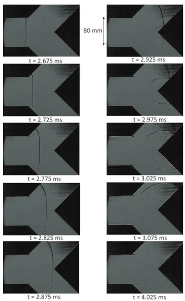
Sets of experiments have been conducted under three dif-ferent Mach numbers and the results are further compared with numerical simulations. The representative experimen-tal schlieren sequences showing the propagation of shock waves having respectively a Mach number of 1.12, 1.36 and 1.69 through the Y-shaped bifurcation are presented in Figs 3, 4 and 5. The incident shock wave initially generated in the main channel of 80×80 mm2square cross section propa-gates from left to right in the ’Y ’ closed device. The time (in milliseconds) appearing on each picture indicates the time that has passed since the incident shock wave reached the C6 station (Fig.1) in the main channel. It should be noted that only the incident shock is represented in the different schlieren sequences, from the area visualization beginning to the end (300 mm diameter circle). That means the two end-wall reflected shocks cannot be seen. Finally, note that we used as window two plates of Plexiglas of 40 mm thick as shown in Fig.1. Then, the optical quality, the thickness and the unperfect parallelism of the plates can be the origin of the dark region in the upper right corner. About lines vis-ible in Figs 3, 4 and 5 it is probably due to the horizontal noise present on the camera sensor and not corrected with the shading procedure.
In Fig.3, during the investigated time, about 1.5 ms, we see the early part of the interaction between the transmit-ted and the reflectransmit-ted shock waves through the bifurcation. Specifically, at t=2.875 ms the incident shock wave reached the peak of the Y-shaped duct. Upon its exit from the shock tube, the incident shock loses its planar shape due to its in-teraction with the expansion waves, located at the two cor-ners of expansion zone, and turns to a curved shock. The expansion zone corresponds to the area between the end of the shock tube main channel and the peak of the Y-shaped duct bifurcation. The expansion waves that we are talking about are generated in this location by the diffraction of the shock wave which leads to the formation of two recircula-tion zones and expansion waves because the pressure de-creases locally. These phenomena will be detailed further. In the considered case (M=1.12) the flow deflection angle, caused by the Y-shaped duct results in a regular reflection; see Fig.3 at t=2.925, 2.975 and 3.025 ms. This will not be the case once the incident shock wave Mach number increases. Finally, the reflected shock wave from the bifurcation go back upstream in the main channel shock tube.
80 mm t = 2.675 ms t = 2.925 ms t = 2.725 ms t = 2.975 ms t = 3.025 ms t = 2.775 ms t = 3.075 ms t = 2.825 ms t = 2.875 ms t = 4.025 ms
Fig. 3 A sequence of schlieren photographs showing an initial planar shock wave, of Mach number of 1.12, propagating from left to right through the ’Y ’ bifurcation.
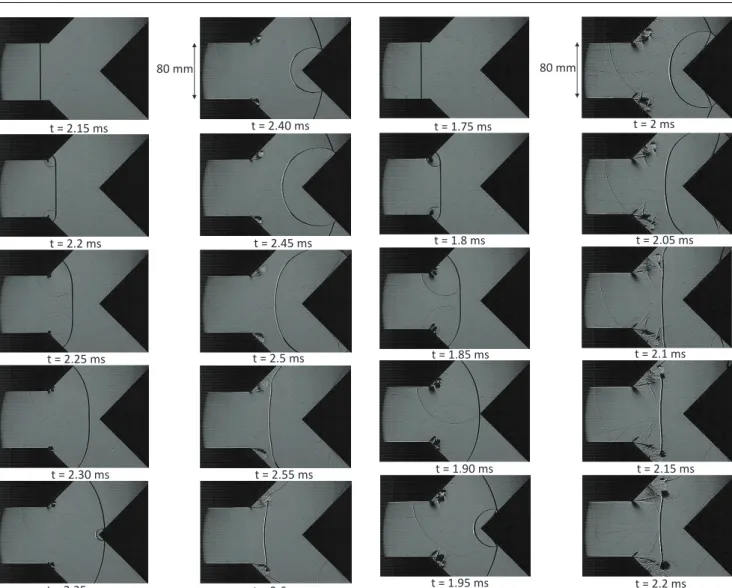
Results shown in Fig.4 are for M=1.36 and it is clear from t=2.40 ms to 2.50 ms, the reflection from the Y-shaped duct is a Mach reflection. More specifically, as shown in Ben-Dor’s work [16], such a reflection is called a single-Mach reflection. The triple point linking the reflected shock wave from the peak of bifurcation, the transmitted shock wave which propagates in the branch and the steam Mach can be seen. Furthermore, in this case, we can observe on the two last pictures the interaction of the shock wave reflected from the Y-shaped duct with the walls. The strong flatten-ing of the reflected shock wave observed from t = 2.5ms to t=2.6ms can be explained by the fact that the shock wave is moving into oncoming flow, but because it is approaching the flow at different angles, that affects its velocity, slower at the symmetry line because it is approaching incoming flow directly while at the two corners, it is at an angle. Thus, the shock wave is stretched out becoming more planar. At t=2.6
80 mm t = 2.15 ms t = 2.40 ms t = 2.2 ms t = 2.45 ms t = 2.5 ms t = 2.25 ms t = 2.55 ms t = 2.30 ms t = 2.35 ms t = 2.6 ms
Fig. 4 A sequence of schlieren photographs showing an initial planar shock wave, of Mach number of 1.36, propagating from left to right through the ’Y ’ bifurcation.
ms, as for the low Mach number case, the reflected shock wave from the Y-shaped duct is just about to enter the shock tube main channel while the shocks reflected from the upper wall of the Y-shaped duct are progressing toward the lower wall. These three shocks collide with the two centered rar-efaction waves creating a zone of highly non-steady and tur-bulent flow. Such multiple interactions reduces the energy contained in the flow and eventually will reduce the pressure acting on the secondary channel end-wall as will be shown subsequently.
Increasing the incident shock wave Mach number will fur-ther intensify the observed flow field as evident in Fig.5, where the incident shock Mach number is 1.69. Again a Mach reflection is observed (see at t=1.95 ms and t=2 ms). Thereafter the wave pattern is amplificated with respect to that observed in the previous case (in Fig.4). We have to note that, while in the previous two cases both the driver
80 mm t = 1.75 ms t = 2 ms t = 1.8 ms t = 2.05 ms t = 2.1 ms t = 1.85 ms t = 2.15 ms t = 1.90 ms t = 1.95 ms t = 2.2 ms
Fig. 5 A sequence of schlieren photographs showing an initial planar shock wave, of Mach number of 1.69, propagating from left to right through the ’Y ’ bifurcation.
and the driven gases were air, in the present case (M=1.69) the driver gas is helium. Consequently, the sound speed be-ing almost three time higher in helium than in air, the ex-pansion waves reflected from the driver’s end-wall catch up the incident shock wave before it enters in the test section. The usual constant pressure plateau triggered behind a nor-mal shock wave is here different and looks more like a blast wave signal with a peak of pressure followed by a decrease (see Fig.6). Indeed, the constant pressure case is a special case for flow in shock tubes with constant cross section area where the expansion fan has not yet caught up the incident shock wave.
Figure6 represents the superposition of the whole shock tube and the pressure distribution for three different times. Re-spectively, the red, the green and the purple lines correspond to the pressure distribution along the shock tube represented, at the instant of the diaphram rupture, when the shock wave has traveled half part of the driven section and when it reaches
Pressure (bar) Diaphragm C6 0 5.5 4 2 Tube lenght (m) 4 2 1 3
Fig. 6 Numerical signal pressure along the shock tube with helium as driver gas for M=1.69.
the C6 gauge station. We can clearly see the drop of pressure behind the shock wave during its propagation. The present case which required Helium as driver gas to experimentally reach a Mach number of 1.69 will not numerically be re-peated in the following where the driver and the driven gases are air.
4.2 Signal pressure evolutions
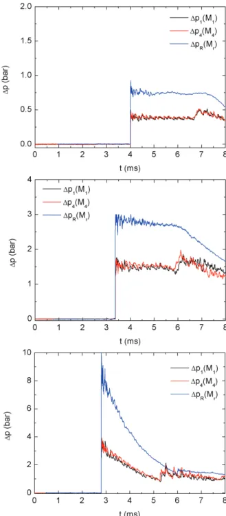
When choosing a special duct geometry for reducing the strength of the transmitted shock, a good way to assess its performance is by comparing the overpressure acting on the closed end-wall (∆P1and∆P4at stations M1and M4) of the considered geometry with a reference defined as that pre-vailing in a similar straight duct (∆Pr in Fig.7.) as schemat-ically shown in Fig.7.
In the investigated channels, pressure gauges M1 and M4 recorded the closed end-wall pressure; obtained results are shown in Fig.8 (black and red line for∆P1and∆P4). It is apparent from this figure that in the cases where the inci-dent shock wave Mach number was either 1.12 or 1.36 the expected constant pressure behind the reflected shock is ev-ident. This is no longer the case when the incident shock wave uses helium as the driver gas (M=1.69).
However, whatever the considered case, it is clear that the pressure acting on the end-wall of a Y-shaped duct is less than half of that acting in a similar end-wall of a straight duct.
M
1
(ΔP
1)
M
4
(ΔP
4)
Mr (ΔPr)
shock shocka)
b)
Fig. 7 Schematic representation of the reference (a) and the Y-shaped duct (b) geometries.
Fig. 8 Overpressure histories recorded behind the reflected shock wave off the end-wall for each branch of the Y-shape section (M1and
M4) compared to that recorded at the end-wall of the main channel
(∆Pr) whitout the test section for Mach numbers of 1.12 (a.), 1.36 (b.) and 1.69 (c.).
4.3 Numerical validation
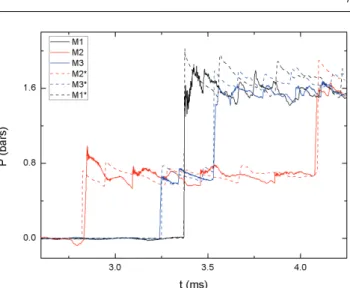
The physical model previously presented is now compared to the experimental results both qualitatively (wave patterns in Fig.9) and quantitatively (pressure signals in Fig.10). Fig.9 presents a comparison of schlieren pictures (experimental versus numerical) taken at same time (corresponding to Fig.4 at t = 2.45 ms). The schlieren variable calculated in the present work is the magnitude of the density gradient computed at each cell and visualized using open source Paraview soft-ware. Specifically, the numerical schlieren is calculated here as follows.
Sn= log10(1 +|
−→
∇ρ|) (7)
In view of the complexity of the present flow in the vicin-ity of the bifurcation, we can reasonably consider the nu-merical calculation in good agreement with the experimen-tal observations. Fig.10, comparisons of pressure signals ob-tained experimentally and numerically for an incident shock wave Mach number of 1.36 are shown for several sensor lo-cations (M1, M2 and M4). Fig.10 shows that no significant difference (less than 5% on the recorded mean value) exists between numerical and experimental pressure traces. Only, the first peak of pressure shows a somewhat larger difference certainly due to the slightly error between the experimental and numerical sensor location. Note that the experimental values of the end-wall reflected pressure are slightly below the numerical ones and can be explained by the non ideal experimental conditions as calibration of sensors, parasistic losses in the device, small leaks or unperfect initial experi-mental condition.
Fig. 9 Numerical (top) and experimental (bottom) schlieren pictures showing the expansion of a planar shock wave through a Y-shaped duct for a Mach number equal to 1.36.
Fig. 10 Comparison of the evolution of the pressure signal in the Y-shape for an incident shock wave Mach number of 1.36 at stations M1,
M2, M3(solid line) and their numerical equivalents noted with ’∗’
(dot-ted line).
4.4 Numerical simulation results
As seen earlier, a flow analysis based on the experimental schlieren photographs (see part 4.1) has been established. Nevertheless, available experimental data do not provide all the necessary information to properly understand the flow field. Indeed, the viewing area is limited to 300 mm and only gives access to the flow wave pattern. In complement to this description, a numerical map of the flow behind the shock wave through the bifurcation has been established, in order to show some complex phenomena which appear with in-creasing velocity of the incident shock wave. Moreover, it can help to answer questions such as, what happens when the incident shock wave passes through the expansion zone? At what incident Mach number the flow behind the shock wave becomes supersonic and does it change the flow havior along the device? Does the incident shock wave be-come planar again after the bifurcation? Numerical calcula-tions allow us to efficiently respond to these quescalcula-tions. It is known that shock diffraction occurs when a plane shock encounters an area increase (expansion) in flow and the de-tails thereof. This can be found in some of the references cited such as [3], [5], [7]. Thus, when the incident shock wave reaches the expansion zone, the flow generates two re-circulation zones, located at the two corners, where the pres-sure is locally reduced and the velocity increased. These re-sults are confirmed in this case in Fig.11.
Now, we focus on the appearance of the first supersonic zone in the flow field behind the incident shock wave to see if it has an impact on the flow behavior. The area of the Y-shaped duct where the flow behavior is the more com-plex is located between the expansion zone and the angle of the bifurcation. Skews’s work [17] describes the behavior of the disturbances produced in the region perturbated behind
Fig. 11 Flow pressure (top, bar) and flow Mach number (bottom) be-hind the shock wave in the expansion zone of the Y device, 2.30 ms after the incident shock wave reaches the C6 station, for a shock wave Mach number of 1.36.
Plot over line « L » L Plot over line «««««««««««««««L««««««««««««««««««««LLLLLLLLLLLLLLLLLLLLLLLLLLLLLLLLLLLLLLLLLLLLLLLLLLLLLLLLLLLLLLLLLLLLLLLLLLLLLLLLLLL»
L L Plot over line “L”
Fig. 12 Scheme of the area studied with the line ’L’ along which the flow field Mach number is calculated
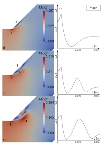
a diffracting shock wave. We are in a similar case of diffrac-tion but only in the very first instant after the incident shock wave enters in the expansion zone because of the bifurcation point acting like an obstacle. At the time when the incident shock wave meets the bifurcation point the problem is no longer the same. As a similar manner we will focus on the appearance behind the incident shock wave of supersonic and subsonic zones in the expansion zone and the bifurcated branch by increasing the incident shock wave Mach number. Thus, we decided to study the evolution of the flow Mach number over time and along a line across this zone as de-scribed in Fig.12. The line ’L’ is placed at 1 mm from the top wall of the bifurcated branch. While the fact that the ve-locity flow behind the incident shock wave increase near the corner is evident (zone ’1’ in Fig.13.a) it is less obvious that this acceleration zone is replaced by two acceleration zones (zones ’3’ and ’4’ Fig.13.c.) separated by a canal of zero speed (zone ’2’ Fig.13. b. and c.). We will see further that these acceleration and zero speed zones will give way to a very complex map of supersonic and subsonic zones in the ’Y ’ device by increasing the Mach number. We conducted
Fig. 13 Zoom of the expansion zone representing the flow Mach num-ber and the corresponding plot along the line ’L’ for an initial Mach number equal to 1.12. for t=2.975 ms (a), 3.325 ms (b) and 3.4 ms (c).
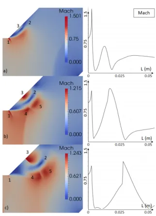
the same study for the two other Mach numbers (1.36 and 1.69). The major difference between the previous case (1.12) and the one explained in Fig 14 (1.36) is that the two accel-eration zones ’1’ and ’3’ are now supersonic as we can see in Fig.14 b. It seems to be important to note that in this case the flow behind the shock wave switch from subsonic to super-sonic by entering the expansion zone. Thus, we have direct transitions between supersonic and subsonic zones, which cannot be possible without the formation of shock waves. We also see in this case the formation of another supersonic zone labelled ’5’ which seems to separate from the zone ’4’ (Fig.14 b. and c.). The flow along the ’L’ line crosses consec-utively two shock waves, twice in a row. Fig.15 represents a numerical sequence of schlieren photographs showing the propagation of the shock wave along the ’Y ’ (Mach 1.36). It is clearly shown the apparition of these shock waves in the expansion zone. Moreover it shows that the reflected shock wave from the point of bifurcation propagates upstream the general flow motion. By increasing the strength of the inci-dent Mach number (1.69), all these mechanisms are repeated and amplified as it is subsequently shown. Fig.16 presents the evolution of the flow Mach number along the line ’L’. We can see that the mechanisms are similar to the previ-ous case (M=1.36) but amplified. The mapping of this area
Fig. 14 Zoom of the expansion zone representing the flow Mach num-ber and the corresponding plot along the line ’L’ for an initial Mach number equal to 1.36. for t=2.45 ms (a), 2.625 ms (b) and 2.875 ms (c). b) e) d) c) a) f)
Fig. 15 Numerical sequence of schlieren photographs, for a shock wave Mach number of 1.36.
shows the flow field is also covered by supersonic and sub-sonic zones separated by shock waves. The zones ’4’ and ’5’ in Fig.16 c. are now separated by another subsonic canal that leads to the formation of a new shock wave allowing the transition between these two supersonic zones. A particular-ity in this case is the border between the zones ’1’ and ’4’ which are both supersonic but whom the transition is
discon-Fig. 16 Zoom of the expansion zone representing the flow Mach num-ber and the corresponding plot along the line ’L’ for an initial Mach number equal to 1.69. for t=2 ms (a), 2.1 ms (b) and 2.2 ms (c).
Fig. 17 Zoom on the expansion zone representing the shocked flow Mach number and the corresponding plot along the line ’L∗’ for an initial Mach number equal to 1.69 (see Fig.16.c.).
tinued as we can see in Fig.17. Indeed, the line along which the flow Mach number is calculated is now shifted in order to cross the zones ’1’, ’4’ and ’5’. The plot of the flow Mach number along the line (’L∗’ located 30 mm away from the top wall) clearly shows the discontinuity between the two supersonic zones (’1’ and ’4’ in Fig.16. c.) and the subsonic canal between ’4’ and ’5’.
In the previous case, for M=1.36, the flow is highly pertur-bated by entering in the expansion zone and because of the reflection of the incident shock wave on the bifurcation point but none of these phenomena remains stationary. It is not the
b) e) d)
c) a)
f)
Fig. 18 Numerical sequence of schlieren photographs for a shock wave Mach number of 1.69.
case for a stronger incident shock wave (M=1.69). Fig.18 presents a numerical sequence of schlieren photographs of the shock wave propagating in the Y shaped duct (M=1.69). We can observe in the expansion zone the creation of quasi-stationary shock waves.
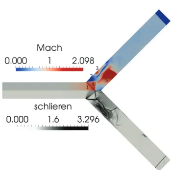
Indeed, in the previous case (M=1.36) the reflected shock wave from the bifurcation point could move upstream, but now it is no longer the case. We clearly see that this reflected shock wave is now stuck in the expansion zone and station-ary, as with the other shock waves present in the flow. Fig.19 corresponds to the superposition of the schlieren den-sity and the Mach number of the flow behind the incident shock wave having a Mach number of 1.69 just before it reaches the end wall. The matching between, the alternately subsonic and supersonic zones and the presence of station-ary shock waves is obvious. Lastly, the incident planar shock wave which curves upon its exit from the shock tube be-comes planar again along the Y branches despite the highly non-steady zones as we can see in Fig.19.
Finally, we have seen that the coupling between the diffrac-tion on the incident shock wave with its reflecdiffrac-tion on the bifurcation point leads to the appearance of acceleration and deceleration zones inside the bifurcation. These zones be-come at first subsonic and supersonic by increasing the in-cident shock wave (M=1.36) and seem to become almost stationary by further increasing the Mach number (1.69).
4.5 Parametric study - Influence of the angular variation As shown in Figs.9 and 10, a very good agreement exists between experimental records and the simulations when the angleα between the shock tube main channel axis and the bifurcation duct, is equal to 45◦(see Fig.20). Therefore, a
1 3
4 2
5
Fig. 19 Numerical superposition of the schlieren density and the flow Mach number just before the incident shock wave (M=1.69) reaches the end wall.
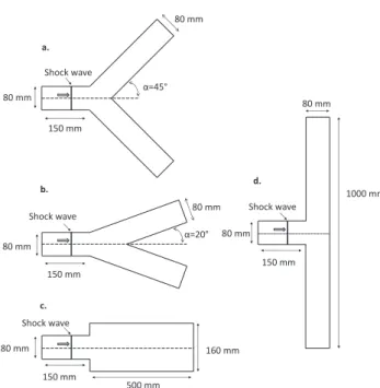
numerical parametric study has been realized by changing respectively α from 90◦ to 0◦ (90◦, 45◦, 20◦, 0◦) which corresponds in this last case to an abrupt opening of the straight duct as schematically represented in Fig.20. The ge-ometry of the abrupt area change configuration was chosen in keeping the same study volume than with the Y-shaped one and keeping the same expansion area ratio equal to two. This analysis which compares for the four geometries the pressure behind the end-wall reflected shock wave, indicates that the change ofα has almost no influence on the pres-sure. It appears that the end-wall reflected pressure calcu-lated in each geometry and for the three Mach numbers stud-ied (1.12, 1.36 and 1.69) are nearly identical as presented in Table1.
500 mm 160 mm 80 mm α=45° α=20° a. c. b. 150 mm Shock wave 80 mm 80 mm 80 mm d. 1000 mm 80 mm 150 mm 80 mm Shock wave Shock wave Shock wave 80 mm 150 mm 150 mm
Fig. 20 Schematic drawing of the numerical devices for the parametric study.
End-wall reflected overpressure (bar) Mach Numbers (a.) 45◦ (b.) 20◦ (c.) 0◦ (d.) 90◦
1.12 0.475 bar 0.480 bar 0.482 bar 0.414 bar 1.36 1.670 bar 1.707 bar 1.730 bar 1.612 bar 1.69 4.349 bar 4.459 bar 4.485 bar 4.339 bar Table 1 Numerical end-wall reflected overpressures for the three ge-ometries and for shock wave Mach numbers 1.12, 1.36 and 1.69.
Thus, the present results clearly show that the angle of the bifurcation has no impact on the end-wall reflected pressure and then on the attenuation of a shock wave propagating through a ducts system. A conclusion which can directly be drawn from this investigation is that the leading parameter which strongly impacts the attenuation of the incident and the reflected shock wave is the enlargement of section and not necessarily the complexity of the duct geometry. Indeed, in all the configurations explored here we have an increase in the cross-section area with a ratio equal to two, which leads to highly reduce the reflected pressure in comparison with the case of a shock wave propagating in a straight shock tube at same condition (see part 4.2). But the value of this attenuation is practically the same in each case and confirms that the expansion ratio of the section area is the preponder-ant parameter compared to the propagation way of the shock wave. Note that experiments with an abrupt opening config-uration (case c. in Fig.20) were also conducted and results obtained also show a very good agreement with the numer-ical simulations as shown in Fig.21 for an incident shock wave Mach number of 1.44.
Fig. 21 Comparison of the experimental and numerical overpressure histories recorded behind the reflected shock wave off the end-wall for the abrupt opening configuration and for an incident shock wave Mach number of 1.44. The red and the black lines correspond to the experimental and the numerical records, respectively.
5 Conclusion
The flow field and the wave patterns developed inside a Y-shaped duct connected to the end of a conventional the shock tube was both experimentally and numerically studied. A detailed description of the wave pattern is given for three dif-ferent Mach numbers. It is shown that very good agreement exists between recorded wave evolvement and their simu-lation; as well as between recorded pressure histories and appropriate simulations. Therefore, the presently used phys-ical model and its numerphys-ical solution could safely be used for similar ducts to be proposed for shock/blast wave atten-uation. The numerical tool allowed us to establish a map of the flow field behind the incident shock wave in order to de-scribe some main physical mechanisms not available in the experimental investigation as the appearance of supersonic zone in the expansion area. It is shown that the pressure pre-vailing behind the reflected shock wave from the end-wall of the Y-shaped duct is less than half of what exists behind a reflected shock wave from a similar straight duct under the same initial conditions. Thereby such duct geometry is a suitable proposal for significantly reducing the potential danger damage of a travelling shock blast wave in tunnels. Moreover, we also have seen that the expansion ratio of the cross-section area is a preponderant parameter in attenuating the strength of a shock wave compared to the duct geometry.
Acknowledgements The project leading to this publication has re-ceived funding from Excellence Initiative of Aix-Marseille University - A∗MIDEX, a French ’Investissements d’Avenir’ program. It has been carried out in the framework of the Labex MEC.
References
1. Ben-Dor G., Igra O., Elperin T.: Handbook of Shock Waves. Aca-demic Press, New York, (2000).
2. Igra O., Wu X., Falcovitz J., Meguro T., Takayama K., Heilig W.: Experimental and theoretical studies of shock wave propagation through double-bend ducts. J. Fluid Mech. 437, 255-282, (2001). 3. Chester W.: The propagation of shock waves in a channel of
non-uniform width. Quart. J. Mech. Appl. Math. 6, 440, (1953). 4. Laporte O.: On interaction of a shock with constriction. Los Alamos
Sci. Lab. Rep. LA 1740, (1954).
5. Chisnell F.: The Normal Motion of a Shock Wave through a non-Uniform One-Dimensional Medium. Proc. Roy. Soc. Lond., 223, 350-370, (1955).
6. Whitham B.: On the propagation of shock waves through regions of non-uniform area or flow. J. Fluid Mech. 4, 337-360, (1958). 7. Nettleton M.A.: Shock attenuation in a ’gradual’ area expansion. J.
Fluid Mech. 60, part 2, 209-223, (1973).
8. Salas M.D.: Shock wave interaction with an abrupt area change, Applied Numerical Mathematics. 12, 239-256, (1993).
9. Igra O., Elperin T., Falcovitz J., Zmiri B.: Shock wave interaction with area changes in ducts. Shock Waves. 3, 233-238, (1994). 10. Heilig W.H.: Propagation of shock waves in various branched
ducts. (ed. G. Kamimoto.) Modern Developments in Shock Tube Research, 273-283. Shock Tube Research Society, Japan, (1975). 11. Skews B.W.: The propagation of shock waves in a complex tunnel
system, Atr. Inst. Min. Metal, 91, no. 4, 137-144, (1991). 12. Igra O., Falcovitz J., Reichenbach H., Heilig W.: Experimental and
numerical study of the interaction between a planar shockwave and a square cavity. J. Fluid Mech. 313, 105-130, (1996).
13. Igra O., Wang L., Falcovitz J., Heilig W.: Shock wave propagation in a branched duct. Shock Waves. 8, 375-381, (1998).
14. Jourdan G., Houas L., Schwaederle L., Layes G., Carrey, Diaz F.: A new variable inclination shock tube for multiple investigations. Shock Waves. 13, 501-504, (2004).
15. Thevand N., Daniel E., Loraud J.C.: On high resolution schemes for compressible viscous two-phase dilute flows; Int. J. Numer. Meth. in Fluids. 31, 681-702, (1999).
16. Ben-Dor G., Shock wave reflection phenomena, Springer, 46-52, (1992).
17. Skews B.W.: The perturbed region behind a diffracting shock wave, Journal of Fluid Mechanics, vol. 29, part 4, pp. 705-719, (1967).