Rule 110: universality and catenations

HAL Id: hal-00273995

https://hal.archives-ouvertes.fr/hal-00273995

Submitted on 16 Apr 2008

HAL is a multi-disciplinary open access archive for the deposit and dissemination of sci-entific research documents, whether they are pub-lished or not. The documents may come from teaching and research institutions in France or abroad, or from public or private research centers.

L’archive ouverte pluridisciplinaire HAL, est destinée au dépôt et à la diffusion de documents scientifiques de niveau recherche, publiés ou non, émanant des établissements d’enseignement et de recherche français ou étrangers, des laboratoires publics ou privés.

Gaétan Richard

To cite this version:

Gaétan Richard. Rule 110: universality and catenations. JAC 2008, Apr 2008, Uzès, France. pp.141-160. �hal-00273995�

GA´ETAN RICHARD Laboratoire d’informatique fondamentale de Marseille (LIF), Aix-Marseille Universit´e, CNRS;

39 rue Joliot-Curie, 13 453 Marseille, France

E-mail address: gaetan.richard@lif.univ-mrs.fr

Abstract. _{Cellular automata are a simple model of parallel computation. Many people} wonder about the computing power of such a model. Following an idea of S. Wolfram [16], M. Cook [3] has proved than even one of the simplest cellular automata can embed any Turing computation. In this paper, we give a new high-level version of this proof using particles and collisions as introduced in [10].

Introduced in the 40s by J. Von Neumann as a parallel model of computation [13], cellular automata consist of many simple entities (cells) disposed on a regular grid. All cells evolve synchronously by changing their state according to the ones of their neighbours. Despite being completely known at the local level, global behavior of a cellular automaton is often impossible to predict (see J. Kari [6]). This comes from the fact that even “simple” cellular automata can exhibit a wide range of complex behaviors. Among those behaviors, one often refers as emergence the fact that “complexity” of the whole system seems far greater than complexity of its elements.

Elementary cellular automata are an example of subclass of “simple” cellular automata. They are obtained by considering only a one dimensional grid (i.e., a line of cells), two possible states and nearest neighbours (i.e., left and right one in addition to the cell itself). Although very restrictive, some elements of this class do exhibit very complex behaviors including emergence. One way to assert such a claim is to prove that some of those cellular automata can embed any Turing computation. Among elementary cellular automata, more likely candidate to this property were though to be the ones that exhibit meta-structures with predictable behavior. Those meta-structures have been studied with regards to their combinatorial aspect (see N. Boccara et al. [1] or J. P. Crutchfield et al. [5]) and widely used as support for constructions. In fact, M. Cook [3] managed to embed any Turing computation in an elementary cellular automaton (namely rule 110) using these structures. However, lack of formalism to manipulate those meta-structures forced him to develop long and complex combinatorial arguments to prove that intuition on behavior is correct.

In this paper, we shall use a new formalism on these meta-structures developed in [10] to provide a complete and high-level proof of Turing universality of rule 110 without the need of complex combinatorial arguments.

2000 ACM Subject Classification: 68Q80,68Q05,37F99.

Key words and phrases: Cellular automata, particles and collisions, Turing, simulation.

c

In section 1, we give formal definitions of cellular automata, discuss about the notion of Turing simulation and introduce the framework of particles and collisions. In section 2, we introduce the cyclic Post tag system (CPTS) used as an intermediate and prove this system is able of any Turing computation. Finally, In section 3, we explicitly give the meta-structures used, present in details the construction to encode CPTS and prove that the encoding method is valid.

1. Cellular automata

Cellular automata are a parallel computation model on a regular grid in discrete time. In general, this model is known to be able of any Turing computation. In this paper, we consider only a very simple subclass of cellular automata: elementary cellular automata (ECA). These automata are made of a line of cells with a binary state {0, 1} and only take into account the three nearest neighbours (i.e., left, center and right). An elementary cellular automaton is thus a function f : {0, 1}3 → {0, 1} also called local transition function. One can notice that this class has only a finite number (256) of elements. Usually, those elements are referred by their index which is the integer obtained by taking for the i-th digit f (i0, i1, i2) where i0i1i2 is the writing of i in base 2. In the rest of the paper, we focus

on rule 110 whose transition function is given on Table 1.

f (l, c, r) 0 1 1 0 1 1 1 0

(l, c, r) (1, 1, 1) (1, 1, 0) (1, 0, 1) (1, 0, 0) (0, 1, 1) (0, 1, 0) (0, 0, 1) (0, 0, 0)

Table 1: Local transition function of rule 110 ECA act, in a synchronous way, over configurations c ∈ {0, 1}Z

by the global transition function F (c)i = f (ci−1, ci, ci+1). Starting from an initial configuration c0, the sequence

of successors O = (F(i)(c0))i∈N is called the orbit starting from c0. To draw an orbit of a

cellular automaton, a convenient method it to pill up elements of this orbit leading to a space-time diagram (see Figure 1).

Figure 1: Example of a space-time diagram of rule 110 (time goes from bottom to top) Due to the parallel nature of cellular automata, they have several differences with other computation models. Therefore, the notion of simulation is less straightforward than usual. Thus, it needs some discussions presented in the following.

1.1. Universalities

Among the differences between cellular automata and other systems, main ones are that they have no halting condition and act on infinite configurations. These two points make it very difficult to achieve a “natural” or even standard definition of simulation by cellular automata of other systems (and in particular Turing machines). In this section, we discuss the notion of Turing universality and present the version used in this paper.

To make a parallel between Turing machines and cellular automata, we first need to introduce some “halting” condition somewhere in cellular automata. This is generally achieved by seeking a particular word in the configuration. This seek can be done ei-ther at a specific place or anywhere on the configuration. Here, we choose the latter option leading to the following formal definition: A word w ∈ {0, 1}∗ _{occurs in an orbit O if there}

exists t ∈ N and x ∈ Z such that w = Ot,xOt,x+1. . . Ot,x+|w|−1.

For input, one solution is to restrict to finite configurations (i.e., configurations with a finite number of non 0 letters). However, this definition is too restrictive in our case. Therefore we prefer to use the less restrictive set of ultimately periodic configurations: that is configurations which are of the formω_lmrω _{where l, m and r are finite words. We request}

that these words can be easily computed from the input word of the Turing machine and that the resulting configuration “halts” if and only if the Turing machine halts. All those points can be formalized in the following definition:

Definition 1.1. A cellular automaton is Turing universal is for any Turing machine M, there exists a word w and a log-space function f which maps any words s ∈ Σ∗ to three words ls, ms, rs such that w occurs in the orbit starting from configurationωlsmsrωs if and

only if M eventually halts on s.

One can note that our definition is a specific case of the more general scheme presented by B. Durand and Zs. R´oka in [4].

Since most of the problems encountered with definitions of Turing universality come from the fact that we deal with two heterogeneous systems, another sensible approach of simulation is to focus on simulation of cellular automata by cellular automata, as described by N. Ollinger in [8]. This idea led to the notion of intrinsic universality. Intuitively, a cellular automaton simulates another one if the space-time diagram of the simulating one can be regularly embedded into the simulating one. Due to the fact that intrinsic universality requires the whole computation to be embedded in a regular way, intrinsic universality implies Turing universality but the converse is false. A more detailed study of those two types of universalities can be found in the survey made by N. Ollinger [9]. In this paper, we deal with the Turing universality of rule 110, the question of intrinsic universality of such a rule is still open.

Theorem 1.2 (M. Cook [3]). Rule 110 is Turing-universal.

The construction made by M. Cook makes heavy use of regular structures present in rule 110. However, due to a lack of specific formalism, it fail to achieve the proof on these structures level and must default to a technical combinatorial approach. In this paper, we intend to lever the proof by using specific high-level tools on these meta-structures. These meta-structures and tools are presented in the next part.

1.2. Particles and collisions

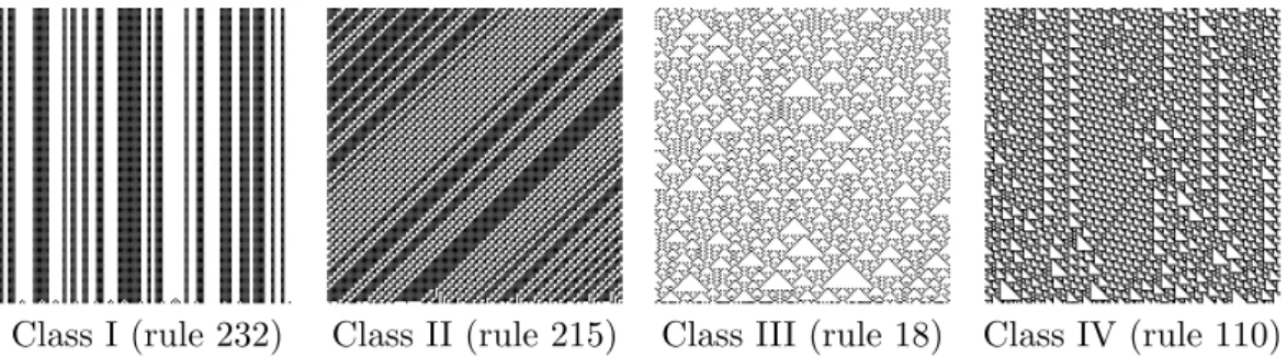
Through very restricted, elementary cellular automata can exhibit a wide range a be-haviors. Those behaviors have been experimentally categorised by S. Wolfram [15] into four classes (see Figure 2): Class I regroups cellular automata whose behavior converges towards a stable configuration. Class II is constituted by those whose orbits ultimately go into a cycle. Class III regroups the ones whose behavior seems random and does not exhibit any kind of regularity. At last, elements of class IV are cellular automata where “(...) local-ized structures are produced which on their own are fairly simple, but these structures move around and interact with each other in very complicated ways. (...)”. Such phenomenon is often referred as self-organisation and is though to include a great computational power. In fact, simulation of Turing machine by rule 110 heavily relies on such structures. To use those structures, we need a formalism as the one introduced in [10] which gives us a formal support on intuitive tools.

Class I (rule 232) Class II (rule 215) Class III (rule 18) Class IV (rule 110) Figure 2: Behaviors of elementary cellular automata

Intuitively, those elements (which can be seen in the last class on Figure 2) can be easily described: most of the space-time diagram is filled with a bi-periodic pattern called background (Figure 3a). Among backgrounds, some uni-periodic structures called particles seem to travel (Figure 3b). These particles interact with each other and give birth to new particles in collisions (Figure 3c).

(a) Background (b) Particle (c) Collision

Figure 3: Examples of elements present in self-organisation and symbolic representation. To give a formalism of these object, one heavily relies on two-dimensional aspect of time diagram. Therefore, in the rest of the paper, we only consider bi-infinite space-time diagrams (i.e., orbits with an infinite sequence of predecessors). Moreover, all defini-tions are based on discrete two-dimensional geometry. In this vision, space-time diagrams are elements of {0, 1}Z2

A coloring is an application C from a subset Sup(C) of Z2 _{to {0, 1}. If Sup(C) is}

finite then the coloring is said to be finite. Restriction of a coloring C to a subset S of Z2 _{is denoted as C|S. Translation of a coloring along a vector u is the coloring of support} {s + u|s ∈ sup(C)}, defined by (u · C)(z + u) = C(z). Disjoint union of two colorings C and C′ whit Sup(C) ∩ Sup(C′) = ∅ is defined such that z ∈ Sup(C), it holds C ⊕ C′(z) = C(z) and for all z ∈ Sup(C′_{), it holds C ⊕ C}′_{(z) = C}′_(z).

A background is a triplet B = (C, u, v) where u, v are two non-collinear elements of Z2 and C a finite coloration satisfying that L_i,j∈Z2(iu + jv) · C is a space-time diagram. In

the rest of the paper, we abusively also denote by B the resulting space-time diagram. A particle is a tuple P = (C, u, Bl, Br) where C is a finite coloring, u ∈ Z2, Bl and Br are

backgrounds, provided that I =L_k∈Zku · C separate the plan in two 4-connected zone L and R (oriented according to u) ensuring that B_|L ⊕ I ⊕ B′

|R is a space-time diagram1.

At last, a collision is a pair (C, L) where C is a finite coloring, L is a finite sequence of n particles Pi = (Bi, Ci, ui, B′i), satisfying:

(1) ∀i ∈ Zn, B′i= Bi+1;

(2) I = C ⊕L_i∈Zn,k∈Nkui· Ci cut the plan in n 4-connected zones;

(3) For all i ∈ Zn, C ⊕L_k∈N(kui· Ci⊕ kui+1· Ci+1) cut the plane in two 4-connected

zones. Let Pi be the one right of Pi;

(4) C = I ⊕L_iBi|Pi is a space-time diagram.

Since finite colorings involved in particles and in collisions can be quite large, it would be unreadable to give them in an analytic form. That’s why we depict them using a graphical version. To help the reader convince itself, rather than just depicting the coloring, we give the finite coloring “in context” and highlight it. This representation is more intuitive but nevertheless completely defines the object. In this paper, all background, particles and collisions shall be given this way (see figure 3). For collisions, we also give the name of involved particles.

The idea behind formalism [10] is to manipulate space-time diagram representing par-ticles as lines and collisions as points. Such representation allows to represent evolutions of the cellular automaton as a planar map (see for example Figure 15) and is formalized below:

Definition 1.3. a catenation scheme is a planar map whose vertices are labeled by collisions and edges by particles which are coherent with respect to collisions.

A catenation scheme is a high-level symbolic assembly of particles and collisions. To make this scheme correspond to a valid space-time diagram, one needs to give explicit positions for every vertex and check that all local constrains are correct. Alternatively, those positions can be given indicating relative position of collisions, for example by specifying the number of repetitions of particles. Such set of repetitions is called valid affectation is the resulting object is a space-time diagram. The main point is that, from a catenation scheme, one can automatically know the form of the set of valid affectations.

Theorem 1.4 ([10]). Given a finite catenation scheme, the set of valid affectations is a computable semi-linear set.

1_{In an exact version, disjoint union is replaced by patchwork which require the different colorings to have}

a “safety border” on which they agree. This condition can be easily fulfilled by making the finite coloring larger. In this paper, we stick to this simplified version.

Catenations allow us to construct complex behaviors for cellular automata exhibiting self-organisation. To apply this in the case of rule 110, we need to manually extract a set of particles and collisions and then use it to simulate our Turing machine. Although rule 110 is known to have a very wide and complex system of particles and collisions, we are still not able to simulate directly a Turing machine. To make the simulation, M. Cook introduces an intermediate dynamical system known as cyclic Post tag systems with several additional constraints. To do this, one must first prove that this system can embed any Turing computation and then that rule 110 can embed this system.

For completeness of the proof, the next section describe how Turing machines can be embedded into this specific version of cyclic Post tag system. On first reading, the reader who is mainly concerned with rule 110 stuff can easily skip this part and just read cyclic Post tag systems definition (def 2.2) and assume the result of proposition 2.4.

2. Cyclic Post tag systems

In this section, we prove that cyclic Post tag systems with additional restrictions can simulate any Turing machine. Those systems are a variant of Post tag systems whose Turing power has been know for long (see H. Wang [14] or J. Cocke and M. Minsky [2]). From those systems, obtaining a cyclic one is not very difficult but ensuring the additional restrictions require a deep understanding of the simulation. Since those restrictions are a key point of the proof of rule 110, we choose to give a full proof of Turing machines simulation.

2.1. Definitions

Introduced by A. Turing in the 30s [12], Turing machines are one of the main dynamical models of computation. In our case, they consist of a bi-infinite tape filled with letters chosen among a finite alphabet Σ (see Figure 4). On the tape, there is a unique head with a state taken among a finite set Q. Dynamics is obtained the following way: at each time step, the head can write a new letter at its position, change its state and make a move to the left or to the right. The behavior of the head is uniquely determined by the current state of the head and the symbol on the tape under it. This behavior is denoted by the transition function δ. Initially, the tape filled with one distinguished white letter w(∈ Σ) on all but a finite portion called input. The head starts at position 0 in the initial state q0 . Computation

steps are done by applying the local rule until the head enters the halting state qf. This

can be formalized with the following definition:

Definition 2.1. A Turing machine (TM for short) is a tuple (Σ, w, Q, q0, qf, δ) where:

• Σ is the finite set of letters; • w ∈ Σ is the white letter; • Q is the finite set of states;

• q0, qf ∈ Q are the initial (resp. halting) state;

• δ : Q × Σ → Q × Σ × {←, →} is the transition function.

At each step, the system is fully defined by a configuration consisting of the non-white portion of the tape along with the current state and position of the head. In this system, all changes are localised under the head. Although simple, this system has as much computational power as most of other known dynamical systems. In this paper, we also use another system known as cyclic Post tag system. This system was first introduced by

w w w w w w w w w w

. . . _{a b a b} . . . _{a w a b} . . .

q _q′

Figure 4: Example of Turing machine transition δ(q, b) = (q′_{, w, →)}

E. Post in 1943 [11]. A Post Tag system (PTS for short) can be described as a finite queue on a finite alphabet Σ. At each step, the system pops a finite fixed number n of letters from the queue. Then, according to the first popped letter, it pushes a (possibly empty) word at the end of the queue (see Figure 5a). The function associating the pushed word to the read letter δ is called transition function. The system starts with an initial finite input word in the queue. Transition rule is applied until there are not enough letters left to pop in the queue (i.e., strictly less than n). Formally, a Post Tag system can be depicted as a triplet (Σ, n, δ) where Σ is the finite set of letters; n is a non-null integer and δ : Σ → Σ∗ is the local transition function.

01 01100 11011 (ǫ, 10011, 011100, 01) 01 100 1011 (10011, 011100, 01, ǫ) 10 0 01110011 (011100, 01, ǫ, 10011) 01 00 11110011 (01, ǫ, 10011, 011100) 00 111001101 (ǫ, 10011, 011100, 01) ǫ (halts) . . .

(a) Post Tag System ({0, 1}, 2, θ) (b) Cyclic Post Tag System

with θ(0) = ǫ and θ(1) = 100 (ǫ, 10011, 011100, 01)

Figure 5: Example of Post tag systems transitions

In this paper, we use a variant of this system, introduced by M. Cook [3], called Cyclic Post Tag System (CPTS for short) depicted in Figure 5b. In this variant, the alpha-bet is fixed to {0, 1} and the transition rule is replaced by a finite cyclic list of words (w0, w1, . . . , wk−1) on {0, 1}∗. At each step, the systems pops the first letter. If this letter

is 1, it pushes the first word of the list (here w0) at the end of the queue. Then, in all cases,

it rotates the list of words — here, for example, the list becomes (w1, w2, . . . , wk−1, w0).

As previously, starting from an initial input word in the queue, transitions occur until the queue is empty. In this case, the system is said to halt on the selected input. This leads to the following definition:

Definition 2.2. A cyclic Post tag system P is a finite cyclic list (w0, w1, . . . , wk−1) of words

over the alphabet {0, 1}.

Once again, at each step, the system can be entirely characterised by a configuration consisting of the current content of the queue and the current rotation of the cyclic list (more precisely, the index of the first word in the list). The rest of this section is devoted to prove that CPTS can embed any Turing machine even when ensuring two additional restrictions. The first one is on the length of every word in the cyclic list. The other one is on the occurrence of letter 1 during any Turing simulation.

2.2. From Turing machines to cyclic Post tag systems

In this section, we show how a CPTS can simulate a Turing machine. Intuitively, the notion of simulation indicates that there exists an easy way to transform any input of the Turing machine into an input of the CPTS such that the Turing machine halts on the input if and only if the CPTS does. This can be formalized by the following:

Definition 2.3. A CPTS P simulates a Turing machine M if there exists a function f : Σ∗ _{→ {0, 1}}∗ _{which is simple}2 _{such that for any word s ∈ Σ}∗_{, M eventually halts on s}

if and only if P eventually halts on f (s).

With this definition, we can state the main theorem of this section which says that a subset of CPTS is sufficient to simulate any Turing machine. As underlined before, the result has been already known for long in the general case but restrictions need a deep understanding of the method used. For this reason and to give the reader a complete view of the embedding process, we give in the following the complete reduction. Restrictions may seem quite mystic by now but they will appear when embedding this system into cellular automaton 110.

Proposition 2.4. Any Turing machine M can be simulated by a cyclic Post tag system P such that:

• the length of any word in P is a multiple of 6;

• during any step of the simulation, there is at most K consecutive steps with 0 as the first popped letter. Moreover, K only depends on M.

Proof. First of all, it is well known than any Turing machine can be simulated by a Turing machine on alphabet {0, 1} with white letter 0. Since the reduction is trivial, we restrict our-selves to Turing machine with this alphabet. In this proof, we prove an even stronger result: there exists a transformation of any Turing machine configurations into CPTS configura-tions which commutes with dynamics. The proof is done by using PTS as an intermediate model.

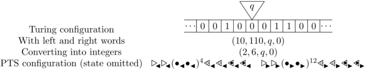
Let us take any Turing machine M = ({0, 1}, 0, Q, q0, qf, δ) and c be a configuration of

the Turing machine. It can be entirely defined by the state of the head q , the portion of the tape on the left of the head, the one on the right and the letter under the head i (see Figure 6). Since left and right words have only a finite number of 1 letters (i.e., non-white), they can be depicted as integers nl and nr which give c on the form (nl, nr, q, i).

At this point, let us how encode this configuration into a PTS (Σ, n, δ′) configuration. To encode all information, we use different methods:

• the left (resp. right) integer is encoded in unary between start and end markers; • state is encoded in every letter of the queue;

• current letter is encoded using the fact that only one letter over n is read.

To allow encoding of all these information, let us take an alphabet Σ0 on the form

M × {◭,◮} × Q × {0, 1} where M = {

⊲

⊳

⊳

one for start, one for interior and two for end). The part {◭,◮} indicates if we speak

about left or right word. the set Q is used to encode the current state. The last part of the alphabet refers to the parity of the position: throughout the construction, every letter on the form (m, f, q, 0) is followed by a (m, f, q, 1) letter. Such sequence is called representation and depicted as mf (omitting the state for clarity). Moreover, representations are often 2_{usually, we request a log-space function but here we use the even more restrictive notion of morphism}

doubled, the result is called tag. With this formalism, a configuration c = (nl, nr, q, 0)

is encoded in the queue as

⊲

⊲

_⊳

◭ ◦

⊳

⊳

⊳

⊲

⊲

r

_⊳

◮ ◦

⊳

⊳

⊳

Figure 6). For the (nl, nr, q, 1) case, the encoding is the same except that the first letter

is removed. As we have made four letters blocs, we choose n = 4 (i.e., read one letter and then discard 3). This ensure that exactly one letter is read per tag.

Turing configuration . . . 0 0 1 0 0 0 1 1 0 0 . . .

q

With left and right words (10, 110, q, 0)

Converting into integers (2, 6, q, 0)

PTS configuration (state omitted)

⊲

⊲

⊳

⊳

⊳

⊳

⊲

⊲

⊳

⊳

⊳

⊳

Figure 6: From Turing machine configuration to PTS configuration

At this point, let us study how transitions are achieved. Let (nl, nr, q, i) be a

config-uration of the Turing machine. Let us assume that the transition is on the form δ(q, i) = (q′_{, s, ←) (the case → is obtained by symmetry). In these conditions, the successor of the}

configuration is (nl/2, 2nr + s, q′, nl mod 2) (shifting bits corresponds to multiplying or

dividing by 2). Thus, in our PTS we need to: • update the state;

• multiply the right value by 2; • add s to the right value; • divide the left value by 2;

• make an integer floor on the left value;

• read the modulus of the left value and transform it into positioning.

Sadly, doing all these operations requires three passes. The current pass is encoded in all letters of the queue by extending the alphabet with a Cartesian product: the new alphabet is Σ1 = Σ0× {A, B, C}. In pass A, we do the first four points. In pass B, we do the floor

and read the modulus and in pass C we convert the read modulus to alignment.

Now, let us construct the transition function achieving this behavior. A full example of transition is given in Figure 7. During pass A, for each encountered tag, we know the current state (present in the letter) and the current value under the head (read in the last element of the letter). Thus we know the transition and can update the state and the left and right values. For the doubled value, we copy the start and end tags, double each interior tag and add one interior case if 1 if written. For the divided value and for each encountered tag (start, interior or end), we write only one corresponding representation (thus dividing the number of letters by two even for boundaries). As the word is only made of tags, the relative position of read letters is the same after the first pass. During pass B, floor and modulus of the divided word are computed as depicted in Figure 7: First, the starting letter is read whereas eating one interior representation and writing a start tag. Thereafter, we write one interior tag for every two interior representations. At the end, we can either arrive on the first or second ending representation according to the interior representation parity. In addition to write both end tags, we can also insert some new letters # to change the relative position in the next step. On other portions, we just need to make a copy which can be easily achieved since they are compound of tags (recall tags are made of four letters and thus are read exactly one time). The last part also consists just of copying. Passing

above letters # ensures the correct new positioning of read letters. A careful reader may note that the depicted method is not fully correct since in pass B, we must know which word must be floored and have no longer access to this information. However, this can be easily overcome by enlarging once again the alphabet.

The last point is to define the behavior in the case we reach an halting state of the Turing machine. This case is easily dealt with by requesting the Post system to erase the whole queue, causing it to halt. To ensure our additional condition, we need to bound the number of step without writing. Since the only case where there is no writing is when erasing the configuration on halting, it is easy to obtain a bound by requesting that the simulated Turing machine halt only with empty tape. This set of machine is obviously also Turing powerful. With this restriction, the number of step without write is bounded by the number of steps (precisely six) to erase the empty configuration

⊲

⊲

⊳

⊳

⊳

⊳

⊲

⊲

⊳

⊳

⊳

⊳

Pass A:

⊲

⊲

⊳

⊳

⊳

⊳

⊲

⊲

⊳

⊳

⊳

⊳

⊲

⊲

⊳

⊳

⊳

⊳

⊲

⊳

⊳

⊲

⊲

⊳

⊳

⊳

⊳

⊲

⊳

⊳

⊲

⊲

⊳

⊳

⊳

⊳

⊲

⊲

⊳

⊳

⊲

⊲

⊳

⊳

⊳

⊳

⊲

⊲

⊳

⊳

⊲

⊲

⊳

⊳

⊳

⊳

⊲

⊲

⊳

⊳

Figure 7: Example of a Turing transition simulation (above is the read queue and below the corresponding elements written).

At this point, we want to convert our PTS system into a CPTS one. This can be done without any real difficulty (see Figure 8). Let us take the alphabet Σ of the PTS. It is possible to represent the n-th letter with a fixed length sequence of 0 by marking a letter 1 in a the n-th position. One can trivially request that the length m of those words is a multiple of 6 (ensuring our first additional condition). This way, we can convert all letters to words on alphabet {0, 1}. Since all letters have the same size, each transition read a fixed number 4m of letters. The transition is indicated by the 1 in the first m read letters. Thus the cyclic list can be done the following way: take a list of length 4m, for the first m words, the word is the result by the transition of the PTS on the m-th letter. All other words are taken empty. To end this, let us look at the maximal number of consecutive erasing. Since a complete rotation of the list correspond to a transition of our PTS, we know there are at most 24m steps without writing.

Initial Post system a ⊢ bb, b ⊢ caa, c ⊢ ǫ

Representation of letters a ⇔ 100000, b ⇔ 010000, c ⇔ 001000

Representation of images bb ⇔ 010000010000, caa ⇔ 001000100000100000, ǫ ⇔ ǫ Cyclic word list (with step 4) (010000010000, 001000100000100000, ǫ, ǫ, . . . , ǫ

| {z }

18×

)

In this transformation, we need to go thorough the configuration three times to simulate one transition of the initial Turing machine. Since we use unary encoding, the length of the configuration can double at each simulated step, thus the speed of simulation suffers an exponential slowdown. With a more subtle and complex methods, T. Neary and D. Woods managed to obtain a polynomial slowdown [7, 17] . This result allows them to obtain stronger results using the simulation presented in the rest of the paper. In particular, they prove that predicting rule 110 is P-complete with respect to Turing reducibility.

3. Universality of rule 110

Now, let us go back to rule 110. This last section is devoted to simulate a CPTS (with the additional restrictions) with rule 110. Of course, this simulation is done using tools introduced in section 1.2. With those tools, the way of constructing and proving the simulation is the following:

(1) First, give an explicit set of particles and collisions of rule 110; (2) Then, construct the simulation at a global level using catenations;

(3) Last, use properties of catenation to ensure that simulation is correct (in particular at local level).

3.1. Particles and collisions of rule 110

Rule 110 do possess a very large number of particles and collisions. In this part, we extract a small subset of those particles and collisions that are used in the construction.

For background, we use only one background (the standard one on rule 110) which is given in Figure 9. Since it is the only background, it is omitted in all following objects and representations.

Figure 9: Background used in the construction (coloring is highlighted)

During the construction, we use a bunch of particles and collisions. To ease the reading and understanding of the construction, some hints about particles and collisions used are given alongside their description.

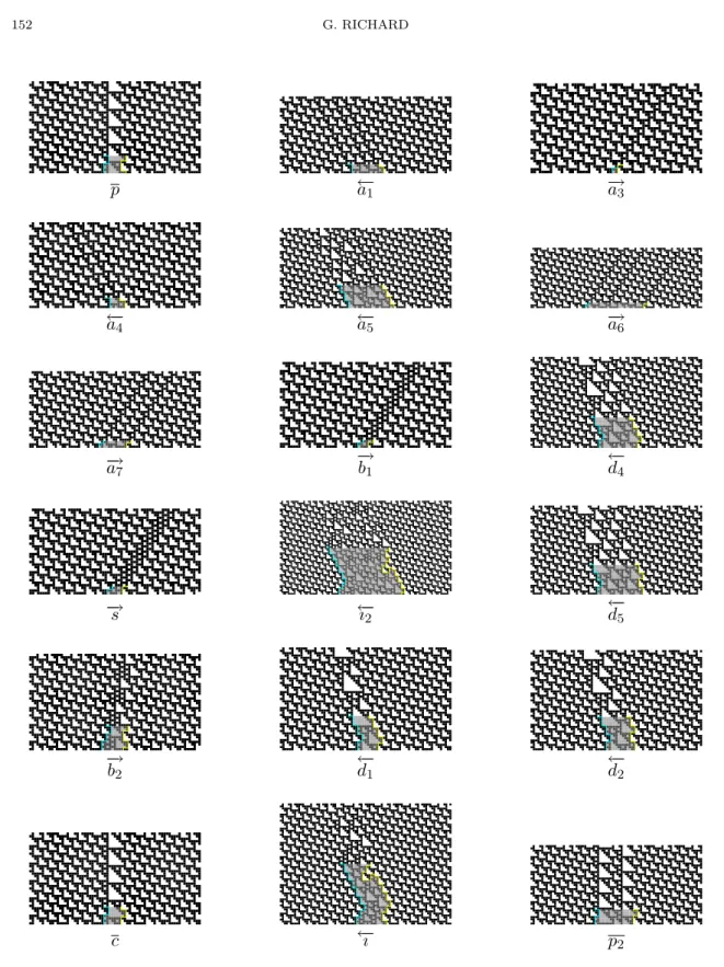
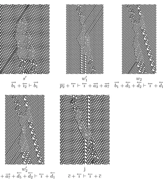
These particles serve as support for information. Dynamic is achieved by a set of 23 collisions depicted in Figures 11 to 13. As for particles, each collision is given by an extract of the space-time diagram where non perturbation pattern is highlighted. Moreover, symbolic behavior of collisions on particles are also given as formulae.

Remark 3.1. The full set of particles and collisions used in this paper contains 18 particles and 23 collisions that are all depicted in Figures 10, 11, 12 and 13.

p ←a−1 −→a3 ←_a− 4 ←a−5 −→a6 − →_a 7 − → b1 ←− d4 − →_s ←_ı− 2 ←− d5 − → b2 ←d−1 ←d−2 c ←−ı p2

f d d′ − → b1 + ←−ı ⊢−→b2 p + ←−ı ⊢ p2 p2+ ←ı−2 ⊢ ←−ı + p f′ _g 1 g2 − → b2 + ←ı−2 ⊢−→b2 c + ←−ı ⊢ ←a−1 c + ←a−1 ⊢ ←−ı + −→a3 g5 g4 g3 − → a3+←d−1 ⊢ p c + ←a−5+ ←a−4 ⊢ ←−ı c + ←−ı ⊢ ←a−5+ ←a−4 + −→a3

g′ 7 g8′ g8 − → a6+ ←−ı ⊢−→b2 −→b2 + ←−ı ⊢−→b1 p2+ ←−ı ⊢−→b2 h g′ 9 g6 − →_{s + ←}−_{ı ⊢ ←}−_{ı + −}→_s −→_b 1 + ←−ı ⊢ p −→a3+ p +←d−4 ⊢ ←−ı + p k s g′ 6 − →_{s + ←}−_{ı ⊢ c} −→_b 2 + ←−ı ⊢−→b1 a→−3+ p +←d−4 ⊢ −→a6

s′ _w′ 1 w2 − → b1 + ←ı−2 ⊢−→b1 p2+ ←−ı ⊢ ←−ı + −→a3+ −a→7 −→b1 +←d−5+←d−2 ⊢ ←−ı +←d−1 w′ 2 j − → a3+ −→a7+←d−5+d←−2 ⊢ ←−ı +←d−1 c + ←−ı ⊢ ←−ı + c

Figure 13: Collisions used in the construction (end)

At this point, let us discuss how to encode CPTS elements using particles. Encoding information into particles can be done in two ways: either by the type of particle used or by the relative position in a group of particles. In the construction, both methods are used. This implies, in particular, that some bits of information are conveyed by groups of parallel particles. Those groups of particles are called symbols and named with capital letters. To encode binary letters of the CPTS, we use groups of four particles, the letter x ∈ {0, 1} is encoded by the relative position of those particles. In the construction different groups are used to encode letters: ←F−x = (←−ı ←ı−2)4 are words list letters (called frozen letters); Cx = c4

are queue letters and ←W−x = ←−ı 4 temporary container (called unfrozen letters). To encode

the cyclic list of words, we also use a starting symbol ←S = ←− −ı ←d−1←d−4←−ı 4←ı−2 and a delimiter

←−

D = ←d−5←d−2←d−1←d−4←−ı 4←−ı . The behavior of transition is stored in a erasing symbol −→B = −→b2 or

a copying symbol P = p. For the dynamic, two additional symbols are needed: a clock −

→

that we denote with a tilde: ˜Fx = (←−ı ←ı−2)3(←−ı ←−ı ), ˜S = ←−ı ←− d1 ←− d4←−ı 4←−ı , ˜D = ←− d5 ←− d2 ←− d1 ←− d4←−ı 4←−ı , ˜ P = −→a3−→a7 and ˜B = − → b1.

Combining collisions into finite catenations, it is possible to obtain 10 different possible behaviors with symbols (and 6 additional with altered versions). The complete list of such catenations are given in Figure 14 and Figure 15. Altered versions are not fully depicted since they can be very easily obtained from non-altered ones. The catenation ˜Cis the same as C with half number of collisions. For ˜S0, the only difference is that the upper collision is

g′₈ rather than f′ (as for ˜M0). For ˜S1 and ˜M1, the same holds replacing the upper collision

d′ by w′₁. The last catenations E0, ˜E0, E1 and ˜E1 are made with only one collision (w2 for

the first two ones, w′

2 for the last two ones).

R −→T +←W−x ⊢ Cx C′ −→T +←J− ⊢ ←−J +−→T C Cx+←W−y ⊢ ←W−y + Cx C˜ Cx+←J ⊢− ←J + C− x S0 C0+←S ⊢− ←−J +→−B S˜0 C0+ ˜S ⊢ ←J + ˜− B S1 C1+←S ⊢− ←−J + P S˜1 C1+ ˜S ⊢ ←J + ˜− P M0 −→B +←F−x ⊢ →−B M˜0 −→B + ˜Fx ⊢ ˜B M1 P +←F−x ⊢ ←W−x+ P M˜1 P + ˜Fx ⊢ ←W−x+ ˜P E0 B +˜ ←D ⊢− ←S− E˜0 B + ˜˜ D ⊢ ˜S E1 P +˜ ←D ⊢− ←S− E˜1 P + ˜˜ D ⊢ ˜S

Figure 14: Local behavior of symbols

3.2. Simulation and catenation

With the previously defined local encoding of CPTS elements, let us proceed by speci-fying the global encoding and construct catenations embedding the dynamic.

Encoding of a CPTS configuration is made the following way: in the center, the queue is written with symbols Cx, the upper symbol of the queue being on the right. Right of

these elements, the cyclic list of words is repeated infinitely starting from the current word. Words are written with symbols ←F−x and separated with symbols

←−

D. The first symbol before the current word is ←S . Furthermore, a symbol is replaced by its altered version− where being the last one before a delimiter — i.e., representing the last letter of a word or being a delimiter (or a start symbol) before an empty word. On the left of the queue contents, there is an infinite amount of −→T symbols.

Proposition 3.2. For any CPTS evolution, it is possible to construct a catenation scheme embedding the evolution.

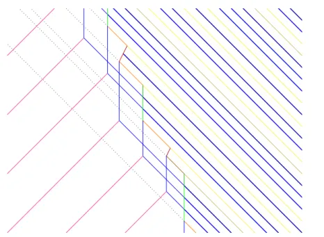
Proof. The catenation uses the symbols presented above. An extract of such a catenation can be found in Figure 16. First, the upper letter of the queue encounters the starting symbol, resulting either on a erasing symbol −→B (catenation S0) or a copying symbol P

(catenation S1) according to the considered letter. This symbol encounters all frozen letters

of the word erasing them (M0) or transforming them into an unfrozen ones (M1). On the

k j j j k j j k j k h h h h h h h h j j j j j j j j j j j j j j j j R C′ C s s′ f f′ s s′ f f′ d d′ d d′ d d′ d d′ g1 g2 g3 g4 g5 g6 d g8 g′ 8 f f′ g1 g2 g3 g4 g5 g′ 6 g₇′ g′₈ g₉′ d d′ M0 M1 S0 S1

Figure 15: Behaviors of symbols

delimiter, transforming it into a new starting symbol (E0 or E1). Unfrozen letters are going

left, crossing all queue letters (C). After that, they are added at the end of the queue when colliding with a−→T symbol (catenation R). One can note that catenations Sx also generate

some junk symbols that go left untouched crossing both queue letters (catenation ˜C) and clock symbols (catenation C). In the case of an empty word, the behavior is the same up to the fact that the altered symbol of copy or erase is directly generated by an altered start catenation ( ˜Sx). After those steps, the system is ready for a new transition. The simulated

system halts when the queue is empty. On the space-time diagram, this condition can be easily expressed by a word indicating that a clock symbol −→T encounters a start of list symbol←S .−

←− W ←− F F˜ ←− S S˜ ←− J ←− D D˜ C P P˜ − → B B˜ − → T

Figure 16: Symbolic behavior of simulation

This explanation conclude the description of dynamic simulation. The last point is to prove that those symbolic behaviors correspond to valid space-time diagrams. At this point, properties of catenation allows us to end the proof without resort to low-level study.

3.3. Validity of simulation

Let us now study the catenation schemes simulating computations of the CPTS. In this section, we shall use properties of catenations to ensure that constructed simulation can really happen in the cellular automaton.

Proposition 3.3. The previously constructed catenations have all valid affectations. More-over, constraints on input are independent on the considered evolution.

Proof. At first, let us look at a global level. Since many symbols are parallel, there are hardly any problem on the order of encounters. The only non-trivial one is that any unfrozen symbols must cross the whole queue before encountering the clock symbol. This implies that is must have crossed the last queue letter before encountering the clock symbols. Since the last queue letter is previous unfrozen letter, the previous condition can be formalized by saying that space between two consecutive clock symbol must be greater than maximum space between two consecutive unfrozen (i.e., copied) letters. At this point, you can see one of the additional conditions on number of consecutive erasing during Turing simulation. With this condition, there is a fixed size for clock spacing ensuring the correct order of collisions independently of the computation.

Now, let us study local constraints. Due to our global approach with collisions and catenations, we have “forgotten” local constraints. In previous proves, the method to ensure these local constraints where by fixing values on the initial configuration and show by induction that they remain consistent. This approach requires a very detailed study and many combinatorial arguments. Here, with the help of catenations, we can have a more global and intuitive approach.

The first remark is that since all our catenations are finite, theorem 1.4 allows us to know affectations such that catenations correspond to real space-time diagram extracts. The set of affectations can be automatically obtained using Presburger arithmetic as described in details in [10].

The only important thing on obtained result is that there exists values for S0 and S1

that have the same spacing for particles inside ←S symbol. The same way, it is possible− to chose fixed values of spacing for all other signal in symbols that ensure coherence in all catenations. The only exception being the junk symbol which has two possibles values depending on whether it has be generated from a S0 or S1 catenation.

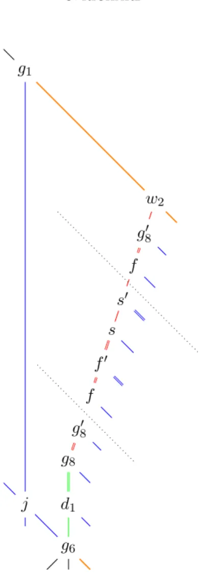
The last point is to study spacing between symbols. During this process, one look at the catenations formed by the border of the one introduced previously. Even if the used method is the same as previously, some interesting things may be noted: First, the main difference between junk signals and unfrozen letters are the relative positions of particles ←−_{ı . Another main point encounter when studying the erasing face (see Figure 17). In this} face, each erased letter induce a small shift which can not be compensated directly. The solution for this problem is to require that the number of letter is a multiple of 6 which provide a greater and solvable gap. This explains the second restriction introduced in our CPTS.

Conclusion

In this paper, we have shown how any Turing computation can be embedded into rule 110. Starting from a Turing machine, we show how to embed it into a CPTS in Proposition 2.4. Then, we show how to encoding this system into rule 110 space-time diagram (Proposition 3.2) and that this encoding is correct (Proposition 3.3). Thus proving that rule 110 is Turing universal. The main achievement is that the construction can be completely made at high level using particles and collisions which allows to follow at each point what is happening. This construction is very interesting but does only erase particles without creating it, thus having the need to be continually feed with particles. This need of “fuel” is not compatible with intrinsic universality. One open question is whether or not rule 110 is intrinsically universal.

References

[1] N. Boccara, J. Nasser, and M. Roger. Particle like structures and their interactions in spatio tempo-ral patterns generated by one-dimensional deterministic cellular-automaton rules. Physical Review A, 44(2):866–875, 1991.

[2] J. Cocke and M. Minsky. Universality of tag systems with p = 2. Journal of the ACM, 11(1):15–20, 1964.

[3] M. Cook. Universality in elementary cellular automata. Complex Systems, 15:1–40, 2004.

[4] B. Durand and Zs R´oka. The game of life: universality revisited. In Cellular automata (Saissac, 1996), pages 51–74. Kluwer Acad. Publ., Dordrecht, 1999.

[5] W. Hordijk, C. R. Shalizi, and J. P. Crutchfield. Upper bound on the products of particle interactions in cellular automata. Physica D, 154(3-4):240–258, 2001.

[6] J. Kari. Theory of cellular automata: a survey. Theoretical Computer Science, 334:3–33, 2005.

[7] T. Neary and D. Woods. P-completeness of cellular automaton rule. In ICALP, Lecture Notes in Com-puter Science, pages 132–143. Springer, 2006.

g6 d1 g8 g₈′ f f′ s s′ f g₈′ w2 j g1

Figure 17: Erasing catenation

[9] N. Ollinger. Universalities in cellular automata; a (short) survey. personal communication (to appear in

JAC 2008), 2008.

[10] N. Ollinger and G. Richard. Collisions and their catenations: Ultimately periodic tilings of the plane. (to appear in the proceedings of IFIP-TCS 2008, available at http://hal.archives-ouvertes.fr/ hal-00175397/en/), 2007.

[11] E. Post. Formal reductions of the general combinatorial decision problem. American Journal of

Math-ematics, 65(2):197–215, 1943.

[12] A. M. Turing. On computable numbers, with an application to the Entscheidungsproblem. Proceedings

of the London Mathematical Society, 2(42):230–265, 1936.

[13] J. Von Neumann. Theory of Self-Reproducing Automata. University of Illinois Press, Urbana, Ill., 1966. [14] H. Wang. Tag systems and lag systems. Mathematische Annalen, 152(1):65–74, 1963.

[15] S. Wolfram. Universality and complexity in cellular automata. Physica D. Nonlinear Phenomena, 10(1-2):1–35, 1984. Cellular automata (Los Alamos, N.M., 1983).

[16] S. Wolfram. A new kind of science. Wolfram Media Inc., Champaign, Ilinois, United States, 2002. [17] D. Woods and T. Neary. On the time complexity of 2-tag systems and small universal Turing machines.

focs, 0:439–448, 2006.

This work is licensed under the Creative Commons Attribution-NoDerivs License. To view a copy of this license, visit http://creativecommons.org/licenses/by-nd/3.0/.