Assessing and tuning brain decoders: cross-validation, caveats, and guidelines

HAL Id: hal-01332785

https://hal.archives-ouvertes.fr/hal-01332785v2

Submitted on 31 Oct 2016

HAL is a multi-disciplinary open access

archive for the deposit and dissemination of

sci-entific research documents, whether they are

pub-lished or not. The documents may come from

teaching and research institutions in France or

abroad, or from public or private research centers.

L’archive ouverte pluridisciplinaire HAL, est

destinée au dépôt et à la diffusion de documents

scientifiques de niveau recherche, publiés ou non,

émanant des établissements d’enseignement et de

recherche français ou étrangers, des laboratoires

publics ou privés.

Distributed under a Creative Commons Attribution| 4.0 International License

Assessing and tuning brain decoders: cross-validation,

caveats, and guidelines

Gaël Varoquaux, Pradeep Reddy Raamana, Denis Engemann, Andrés

Hoyos-Idrobo, Yannick Schwartz, Bertrand Thirion

To cite this version:

Gaël Varoquaux, Pradeep Reddy Raamana, Denis Engemann, Andrés Hoyos-Idrobo, Yannick

Schwartz, et al.. Assessing and tuning brain decoders: cross-validation, caveats, and guidelines.

NeuroImage, Elsevier, 2016, �10.1016/j.neuroimage.2016.10.038�. �hal-01332785v2�

Assessing and tuning brain decoders: cross-validation, caveats, and guidelines

Ga¨el Varoquauxa,b,∗_{, Pradeep Reddy Raamana}d,c_{, Denis A. Engemann}e,b,f_{, Andr´es Hoyos-Idrobo}a,b_{, Yannick}

Schwartza,b_{, Bertrand Thirion}a,b

a_{Parietal project-team, INRIA Saclay-ˆıle de France, France} b_{CEA/Neurospin bˆat 145, 91191 Gif-Sur-Yvette, France}

c_{Rotman Research Institute, Baycrest Health Sciences, Toronto, ON, Canada M6A 2E1} d_{Dept. of Medical Biophysics, University of Toronto, Toronto, ON, Canada M5S 1A1}

e_{Cognitive Neuroimaging Unit, INSERM, Universit´e Paris-Sud and Universit´e Paris-Saclay, 91191 Gif-sur-Yvette, France} f_{Neuropsychology & Neuroimaging team INSERM UMRS 975, Brain and Spine Institute (ICM), Paris}

Abstract

Decoding, ie prediction from brain images or signals, calls for empirical evaluation of its predictive power. Such evaluation is achieved via cross-validation, a method also used to tune decoders’ hyper-parameters. This paper is a review on cross-validation procedures for decoding in neuroimaging. It includes a didactic overview of the relevant theoretical considerations. Practical aspects are highlighted with an extensive empirical study of the common decoders in within-and across-subject predictions, on multiple datasets –anatomical within-and functional MRI within-and MEG– within-and simulations. Theory and experiments outline that the popular “leave-one-out” strategy leads to unstable and biased estimates, and a repeated random splits method should be preferred. Experiments outline the large error bars of cross-validation in neuroimaging settings: typical confidence intervals of 10%. Nested cross-validation can tune decoders’ parameters while avoiding circularity bias. However we find that it can be more favorable to use sane defaults, in particular for non-sparse decoders.

Keywords: cross-validation; decoding; fMRI; model selection; sparse; bagging; MVPA

1. Introduction: decoding needs model evaluation

Decoding, ie predicting behavior or phenotypes from brain images or signals, has become a central tool in neu-roimage data processing [20, 21, 24, 42, 58, 61]. In clin-ical applications, prediction opens the door to diagnosis or prognosis [9, 11, 40]. To study cognition, successful prediction is seen as evidence of a link between observed behavior and a brain region [19] or a small fraction of the image [28]. Decoding power can test if an encoding model describes well multiple facets of stimuli [38,41]. Prediction can be used to establish what specific brain functions are implied by observed activations [48,53]. All these applica-tions rely on measuring the predictive power of a decoder. Assessing predictive power is difficult as it calls for characterizing the decoder on prospective data, rather than on the data at hand. Another challenge is that the decoder must often choose between many different esti-mates that give rise to the same prediction error on the data, when there are more features (voxels) than samples (brain images, trials, or subjects). For this choice, it relies on some form of regularization, that embodies a prior on the solution [18]. The amount of regularization is a pa-rameter of the decoder that may require tuning. Choosing a decoder, or setting appropriately its internal parameters,

∗

Corresponding author

are important questions for brain mapping, as these choice will not only condition the prediction performance of the decoder, but also the brain features that it highlights.

Measuring prediction accuracy is central to decoding, to assess a decoder, select one in various alternatives, or tune its parameters. The topic of this paper is cross-validation, the standard tool to measure predictive power and tune parameters in decoding. The first section is a primer on cross-validation giving the theoretical under-pinnings and the current practice in neuroimaging. In the second section, we perform an extensive empirical study. This study shows that cross-validation results carry a large uncertainty, that cross-validation should be performed on full blocks of correlated data, and that repeated random splits should be preferred to leave-one-out. Results also yield guidelines for decoder parameter choice in terms of prediction performance and stability.

2. A primer on cross-validation

This section is a tutorial introduction to important con-cepts in cross validation for decoding from brain images.

2.1. Cross-validation: estimating predictive power In neuroimaging, a decoder is a predictive model that, given brain images X, infers an external variable y. Typ-ically, y is a categorical variable giving the experimental

condition or the health status of subjects. The accuracy, or predictive power, of this model is the expected error on the prediction, formally:

accuracy = E[E(ypred, yground truth)] (1) where E is a measure of the error, most often1the fraction of instances for which ypred ≠yground truth. Importantly, in equation (1_{), E denotes the expectation, ie the average} error that the model would make on infinite amount of data generated from the same experimental process.

In decoding settings, the investigator has access to la-beled data, ie brain images for which the variable to pre-dict, y, is known. These data are used to train the model, fitting the model parameters, and to estimate its predic-tive power. However, the same observations cannot be used for both. Indeed, it is much easier to find the correct labels for brain images that have been seen by the decoder than for unknown images2. The challenge is to measure the ability to generalize to new data.

The standard approach to measure predictive power is cross-validation: the available data is split into a train set, used to train the model, and a test set, unseen by the model during training and used to compute a prediction error (figure 1). Chapter 7 of [18] contains a reference on statistical aspects of cross-validation. Below, we detail important considerations in neuroimaging.

Independence of train and test sets. Cross-validation re-lies on independence between the train and test sets. With time-series, as in fMRI, the autocorrelation of brain sig-nals and the temporal structure of the confounds imply that a time separation is needed to give truly independent observations. In addition, to give a meaningful estimate of prediction power, the test set should contain new samples displaying all confounding uncontrolled sources of variabil-ity. For instance, in multi-session data, it is harder to pre-dict on a new session than to leave out part of each session and use these samples as a test set. However, generaliza-tion to new sessions is useful to capture actual invariant information. Similarly, for multi-subject data, predictions on new subjects give results that hold at the population level. However, a confound such as movement may corre-late with the diagnostic status predicted. In such a case the amount of movement should be balanced between train and test set.

Sufficient test data. Large test sets are necessary to ob-tain sufficient power for the prediction error for each split of cross-validation. As the amount of data is limited, there is a balance to strike between achieving such large test sets

1_{For multi-class problems, where there is more than 2 categories} in y, or for unbalanced classes, a more elaborate choice is advisable, to distinguish misses and false detections for each class.

2_{A simple strategy that makes no errors on seen images is simply} to store all these images during the training and, when asked to predict on an image, to look up the corresponding label in the store.

Figure 1: Cross-validation: the data is split multiple times into a train set, used to train the model, and a test set, used

to compute predictive power. Train set Test set

Full data

and keeping enough training data to reach a good fit with the decoder. Indeed, theoretical results show that cross-validation has a negative bias on small dataset [2, sec.5.1] as it involves fitting models on a fraction of the data. On the other hand, large test sets decrease the variance of the estimated accuracy [2, sec.5.2]. A good cross-validation strategy balances these two opposite effects. Neuroimag-ing papers often use leave one out cross-validation, leavNeuroimag-ing out a single sample at each split. While this provides am-ple data for training, it maximizes test-set variance and does not yield stable estimates of predictive accuracy3. From a decision-theory standpoint, it is preferable to leave out 10% to 20% of the data, as in 10-fold cross-validation [18, chap. 7.12] [5, 27]. Finally, it is also beneficial to in-crease the number of splits while keeping a given ratio be-tween train and test set size. For this purpose k-fold can be replaced by strategies relying on repeated random splits of the data (sometimes called repeated learning-testing4 _[2] or ShuffleSplit [43]). As discussed above, such splits should be consistent with the dependence structure across the observations (using eg a LabelShuffleSplit ), or the train-ing set could be stratified to avoid class imbalance [49]. In neuroimaging, good strategies often involve leaving out sessions or subjects.

2.2. Hyper-parameter selection

A necessary evil: one size does not fit all. In standard statistics, fitting a simple model on abundant data can be done without the tricky choice of a meta-parameter: all model parameters are estimated from the data, for in-stance with a maximum-likelihood criterion. However, in high-dimensional settings, when the number of model pa-rameters is much larger than the sample size, some form of regularization is needed. Indeed, adjusting model parame-ters to best fit the data without restriction leads to overfit, ie fitting noise [18, chap. 7]. Some form of regularization or prior is then necessary to restrict model complexity, e.g. with low-dimensional PCA in discriminant analysis [7], or by selecting a small number of voxels with a sparse penalty [6, 60]. If too much regularization is imposed, the ensu-ing models are too constrained by the prior, they underfit, ie they do not exploit the full richness of the data. Both underfitting and overfitting are detrimental to predictive power and to the estimation of model weights, the decoder maps. Choosing the amount of regularization is a typical

3_{One simple aspect of the shortcomings of small test sets is that} they produce unbalanced dataset, in particular leave-one-out for which there is only one class represented in the test set.

4_{Also related is bootstrap CV, which may however duplicate} sam-ples inside the training set of the test set.

Figure 2: Nested cross-validation: two cross-validation loops are run one inside the other.

Validation set Full data Test set Train set Nested loop Outer loop Decoding set

bias-variance problem: erring on the side of variance leads to overfit, while too much bias leads to underfit. In gen-eral, the best tradeoff is a data-specific choice, governed by the statistical power of the prediction task: the amount of data and the signal-to-noise ratio.

Nested cross-validation. Choosing the right amount of regularization can improve the predictive power of a de-coder and controls the appearance of the weight maps. The most common approach to set it is to use cross-validation to measure predictive power for various choices of regularization and to retain the value that maximizes predictive power. Importantly, with such a procedure, the amount of regularization becomes a parameter adjusted on data, and thus the predictive performance measured in the corresponding cross-validation loop is not a reliable as-sessment of the predictive performance of the model. The standard procedure is then to refit the model on the avail-able data, and test its predictive performance on new data, called a validation set. Given a finite amount of data, a nested cross-validation procedure can be employed: the data are repeatedly split in a validation set and a decod-ing set to perform decoddecod-ing. The decoddecod-ing set itself is split in multiple train and test sets with the same valida-tion set, forming an inner “nested” cross-validavalida-tion loop used to set the regularization hyper-parameter, while the external loop varying the validation set is used to measure prediction performance –see figure 2.

Model averaging. Choosing the best model in a family of good models is hard. One option is to average the predic-tions of a set of suitable models [44, chap. 35], [8,23, 29] –see [18, chap. 8] for a description outside of neuroimaging. A simple version of this idea is bagging [4]: using bootstrap, random resamplings of the data, to generate many train sets and corresponding models, the predictions of which are then averaged. The benefit of these approaches is that if the errors of each model are sufficiently independent, they average out: the average model performs better and displays much less variance. With linear models often used as decoders in neuroimaging, model averaging is appealing as it boils down to averaging weight maps.

To benefit from the stabilizing effect of model averaging in parameter tuning, we can use a variant of both cross-validation and model averaging5_{. In a standard} cross-validation procedure, we repeatedly split the data in train

5_{The combination of cross-validation and model averaging is not} new (see eg [23]), but it is seldom discussed in the neuroimaging

and test set and for each split, compute the test error for a grid of hyper-parameter values. However, instead of selecting the hyper-parameter value that minimizes the mean test error across the different splits, we select for each split the model that minimizes the corresponding test error and average these models across splits.

2.3. Model selection for neuroimaging decoders Decoding in neuroimaging faces specific model-selection challenges. The main challenge is probably the scarcity of data relative to their dimensionality, typically hundreds of observations6_{. Another important aspect of} decoding is that, beyond predictive power, interpreting model weights is relevant.

Common decoders and their regularization. Both to pre-fer simpler models and to facilitate interpretation, linear models are ubiquitous in decoding. In fact, their weights form the common brain maps for visual interpretation.

The classifier used most often in fMRI is the support vector machine (SVM) [7, 31, 40]. However, logistic re-gressions (Log-Reg) are also often used [7,50,52,57,60]. Both of these classifiers learn a linear model by minimizing the sum of a loss L –a data-fit term– and a penalty p –the regularizing energy term that favors simpler models:

ˆ w = argmin w (L(w) + 1 Cp(w)) L = ⎧ ⎪ ⎪ ⎨ ⎪ ⎪ ⎩ SVM logistic where C is the regularization parameter that controls the bias-variance tradeoff: small C means strong regulariza-tion. The SVM and logistic regression model differ only by the loss used. For the SVM the loss is a hinge loss: flat and exactly zero for well-classified samples and with a mis-classification cost increasing linearly with distance to the

literature. It is commonly used in other areas of machine learning, for instance to set parameters in bagged models such as trees, by monitoring the out-of-bag error (eg in the scikit-learn library [43]).

6_{While in imaging neuroscience, hundreds of observations seems} acceptably large, it is markedly below common sample sizes in ma-chine learning. Indeed, data analysis in brain imaging has histori-cally been driven by very simple models while machine learning has tackled rich models since its inception.

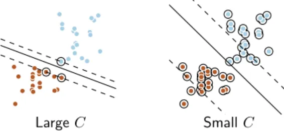
Large C Small C

Figure 3: Regularization with SVM-`2: blue and brown points are training samples of each class. The SVM learns a separating line between the two classes. In a weakly regularized setting (large C, this line is supported by few observations –called support vectors–, circled in black on the figure, while in a strongly-regularized case (small C), it is supported by the whole data.

C=10−5 C=1. Log-reg `1 C=102 C=105 C=10−5 SVM `2 C=1 L R C=105

Figure 4: Varying amount of regularization on the face vs house discrimination in the Haxby 2001 data [19]. Left: with a log-reg `1, more regularization (small C) induces sparsity. Right: with an SVM `2, small C means that weight maps are a combination of a larger number of original images, although this has only a small visual impact on the corresponding brain maps.

decision boundary. For the logistic regression, it is a logis-tic loss, which is a soft, exponentially-decreasing, version of the hinge [18]. By far the most common regularization is the `2 penalty. Indeed, the common form of SVM uses

`2 regularization, which we will denote SVM-`2.

Com-bined with the large zero region of the hinge loss, strong `2penalty implies that SVMs build their decision functions

by combining a small number of training images (see figure 3). Logistic regression is similar: the loss has no flat re-gion, and thus every sample is used, but some very weakly. Another frequent form of penalty, `1, imposes sparsity on

the weights: a strong regularization means that the weight maps w are mostly comprised of zero voxels (see Fig.4). Parameter-tuning in neuroimaging. In neuroimaging, many publications do not discuss their choice of decoder hyper-parameters; while others state that they use the de-fault value, eg C = 1 for SVMs. Standard machine learning practice advocates setting the parameters by nested cross-validation [18]. For non sparse, `2-penalized models, the

amount of regularization often does not have a strong in-fluence on the weight maps of the decoder (see figure 4). Indeed, regularization in these models changes the frac-tion of input maps supporting the hyperplane (see 3). As activation maps for the same condition often have similar aspects, this fraction impacts weakly decoders’ maps.

For sparse models, using the `1penalty, sparsity is

of-ten seen as a means to select relevant voxels for prediction [6, 52]. In this case, the amount of regularization has a very visible consequence on weight maps and voxel selec-tion (see figure 4). Neuroimaging studies often set it by cross-validation [6], though very seldom nested (exceptions comprise [8, 57]). Voxel selection by `1 penalty on brain

maps is unstable because neighboring voxels respond simi-larly and `1estimators will choose somewhat randomly few

of these correlated features [51,57]. Hence various strate-gies combining sparse models are used in neuroimaging to improve decoding performance and stability. Averaging weight maps across cross-validation folds [23, 57], as de-scribed above, is interesting, as it stays in the realm of linear models. Relatedly, [16] report the median of weight maps, thought it does not correspond to weights in a pre-dictive model. Consensus between sparse models over data

perturbations gives theoretically better feature selection [35]. In fMRI, it has been used to screen voxels before fitting linear models [51,57] or to interpret selected voxels [60].

For model selection in neuroimaging, prediction per-formance is not the only relevant metric and some con-trol over the estimated model weights is also important. For this purpose, [30, 50, 55] advocate using a tradeoff between prediction performance and stability of decoder maps. Stability is a proxy for estimation error on these maps, a quantity that is not accessible without knowing the ground truth. While very useful it gives only indi-rect information on estimation error: it does not con-trol whether all the predictive brain regions were found, nor whether all regions found are predictive. Indeed, a decoder choosing its maps independently from the data would be very stable, though likely with poor prediction performance. Hence the challenge is in finding a good prediction-stability tradeoff [50,56].

3. Empirical studies: cross-validation at work

Here we highlight practical aspects of cross-validation in brain decoding with simple experiments. We first demonstrate the variability of prediction estimates on MRI, MEG, and simulated data. We then explore how to tune decoders parameters.

3.1. Experiments on real neuroimaging data

A variety of decoding datasets. To achieve reliable empiri-cal conclusions, it is important to consider a large number of different neuroimaging studies. We investigate cross-validation in a large number of 2-class classification prob-lems, from 7 different fMRI datasets (an exhaustive list can be found inAppendix E). We decode visual stimuli within subject (across sessions) in the classic Haxby dataset [19], and across subjects using data from [10]. We discriminate across subjects i) affective content with data from [59], ii) visual from narrative with data from [39], iii) famous, familiar, and scrambled faces from a visual-presentations dataset [22], and iv) left and right saccades in data from [26]. We also use a non-published dataset, ds009 from

openfMRI [47]. All the across-subject predictions are per-formed on trial-by-trial response (Z-score maps) computed in a first-level GLM. Finally, beyond fMRI, we perform prediction of gender from VBM maps using the OASIS data [34]. Note that all these tasks cover many different settings, range from easy discriminations to hard ones, and (regarding fMRI) recruit very different systems with differ-ent effect size and variability. The number of observations available to the decoder varies between 80 (40 per class) and 400, with balanced classes.

The results and figures reported below are for all these datasets. We use more inter-subject than intra-subject datasets. However 15 classification tasks out of 31 are intra-subject (see Tab.A1). In addition, when decoding is performed intra-subject, each subject gives rise to a cross-validation. Thus in our cross-validation study, 82% of the data points are for intra-subject settings.

All MR data but [26] are openly available from openfMRI [47] or OASIS [34]. Standard preprocess-ing and first-level analysis were applied uspreprocess-ing SPM, Nipype and Nipy (details in Appendix F.1). All MR data were variance-normalized7and spatially-smoothed at 6 mm FWHM for fMRI data and 2 mm FWHM for VBM data.

MEG data. Beyond MR data, we assess cross-validation strategies for decoding of event-related dynamics in neuro-physiological data. We analyze magneteoencephalography (MEG) data from a working-memory experiment made available by the Human Connectome Project [33]. We per-form intra-subject decoding in 52 subjects with two runs, using a temporal window on the sensor signals (as in [54]). Here, each run serves as validation set for the other run. We consider two-class decoding problems, focusing on ei-ther the image content (faces vs tools) or the functional role in the working memory task (target vs low-level and high-level distractors). This yields in total four classifica-tion analyzes per subject. For each trial, the feature set is a time window constrained to 50 ms before and 300 ms after event onset, emphasizing visual components. We use the cleaned single-trial outputs from the HCP “tmegpre-proc” pipeline. MEG data analysis was performed with the MNE-Python software [13, 14]. Full details on the analysis are given inAppendix F.3.

Experimental setup. Our experiments make use of nested cross-validation for an accurate measure of prediction power. As in figure2, we repeatedly split the data in a val-idation set and a decoding set passed on to the decoding procedure (including parameter-tuning for experiments in 3.3 and3.4). To get a good measure of predictive power, we choose large validation sets of 50% of the data, respect-ing the sample dependence structure (leavrespect-ing out subjects,

7_{Division of each time series voxel/MEG sensor by its standard} deviation

or sessions). We use 10 different validation sets that each contribute a data point in results.

We follow standard decoding practice in fMRI [45]. We use univariate feature selection on the training set to select the strongest 20% of voxels and train a decoder on the selected features. As a choice of decoder, we explore classic linear models: SVM and logistic regression with `1 and `2

penalty8. We use scikit-learn for all decoders [1,43]. In a first experiment, we compare decoder performance estimated by cross-validation on the decoding set, with performance measured on the validation set. In a second experiment, we investigate the use of cross-validation to tune the model’s regularization parameter, either using the standard refitting approach, or averaging as described in section2.2, as well as using the default C = 1 choice of parameter, and a value of C = 1000.

3.2. Results: cross-validation to assess predictive power Reliability of the cross-validation measure. Considering that prediction error on the large left-out validation set is a good estimate of predictive power, we use it to as-sess the quality of the estimate given by the nested cross-validation loop. Figure5shows the prediction error mea-sured by cross-validation as a function of the validation-set error across all datavalidation-sets and validation splits. It re-veals a small negative bias: as predicted by the theory,

8_{Similar decoders adding a regularization that captures} spatio-temporal correlations among the voxels are well suited for neuroimag-ing [15,16,25,36]. Also, random forests, based on model averaging discussed above, have been used in fMRI [29,32]. However, this re-view focuses on the most common practice. Indeed, these decoders entail computational costs that are intractable given the number of models fit in the experiments.

50.0% 60.0% 70.0% 80.0% 90.0% 100.0%

Decoder accuracy on validation set 

50.0% 60.0% 70.0% 80.0% 90.0% 100.0%

Decoder accuracy 

measured by cross­validation

Intra subject Inter subject

Figure 5: Prediction error: cross-validated versus validation set. Each point is a measure of predictor error in the inner cross-validation loop (10 splits, leaving out 20%), or in the left-out vali-dation set. The dark line is an indication of the tendency, using a lowess local regression. The two light lines indicate the boundaries above and below which fall 5% of the points. They are estimated using a Gaussian kernel density estimator, with a bandwidth set by the Scott method, and computing the CDF along the y direction.

Cross-validation Difference in accuracy measured strategy by cross-validation and on validation set

­40% ­20% ­10%  0% +10% +20% +40% Leave one sample out Leave one subject/session 20% left­out,   3 splits 20% left­out,   10 splits 20% left­out,   50 splits ­22% +19% +3% +43% ­10% +10% ­21% +17% ­11% +11% ­24% +16% ­9% +9% ­24% +14% ­9% +7% ­23% +13%   Intra subject   Inter subject cross-validation < validation set cross-validation > validation set

Figure 6: Cross-validation error: different strategies. Dif-ference between accuracy measured by cross-validation and on the validation set, in intra and inter-subject settings, for different cross-validation strategies: leave one sample out, leave one block of samples out (where the block is the natural unit of the experiment: subject or session), or random splits leaving out 20% of the blocks as test data, with 3, 10, or 50 random splits. For inter-subject settings, leave one sample out corresponds to leaving a session out. The box gives the quartiles, while the whiskers give the 5 and 95 percentiles.

cross-validation is pessimistic compared to a model fit on the complete decoding set. However, models that perform poorly are often reported with a better performance by cross-validation. Additionally, cross-validation estimates display a large variance: there is a scatter between esti-mates in the nested cross-validation loop and in the vali-dation set.

Different cross-validation strategies. Figure6summarizes the discrepancy between prediction accuracy measured by cross validation and on the validation set for different cross-validation strategies: leaving one sample out, leaving one block of data out –where blocks are the natural units of the experiment, sessions or subjects– and random splits leaving out 20% of the blocks of data with 3, 10, and 50 repetitions.

Ideally, a good cross-validation strategy would mini-mize this discrepancy. We find that leave-one-sample out is very optimistic in within-subject settings. This is ex-pected, as samples are highly correlated. When leaving out blocks of data that minimize dependency between train and test set, the bias mostly disappears. The remaining discrepancy appears mostly as variance in the estimates of prediction accuracy. For repeated random splits of the data, the larger the number of splits, the smaller the vari-ance. Performing 10 to 50 splits with 20% of the data blocks left out gives a better estimation than leaving suc-cessively each blocks out, at a fraction of the computing cost if the number of blocks is large. While intra and

Cross-validation Difference in accuracy measured strategy by cross-validation and on validation set

­40% ­20% ­10%  0% +10% +20% +40% Leave one sample out Leave one block out 20% left­out,   3 splits 20% left­out,   10 splits 20% left­out,   50 splits ­16% +14% +4% +33% ­15% +13% ­8% +8% ­15% +12% ­10% +11% ­13% +10% ­8% +8% ­12% +10% ­7% +7% MEG data Simulations cross-validation < validation set cross-validation > validation set

Figure 7: Cross-validation error: non-MRI modalities. Dif-ference between accuracy measured by cross-validation and on the validation set, for MEG data and simulated data, with different cross-validation strategies. Detailed simulation results inAppendix A.

inter subject settings do not differ strongly when leav-ing out blocks of data, intra-subject settleav-ings display a larger variance of estimation as well as a slight negative bias. These are likely due to non-stationarity in the time-series, eg scanner drift or loss of vigilance. In inter-subject settings, heterogeneities may hinder prediction [56], yet a cross-validation strategy with multiple subjects in the test set will yield a good estimate of prediction accuracy9. Other modalities: MEG and simulations. We run the ex-periments on the MEG decoding tasks and the simulations. We generate simple simulated data that mimic brain imaging to better understand trends and limitations of cross-validation. Briefly, we generate data with 2 classes in 100 dimensions with Gaussian noise temporally auto-correlated and varying the separation between the class centers (more details inAppendix A). We run the exper-iments on a decoding set of 200 samples.

The results, displayed in figure7, reproduce the trends observed on MR data. As the simulated data is tempo-rally auto-correlated, leave-one-sample-out is strongly op-timistic. Detailed analysis varying the separability of the classes (Appendix A) shows that cross-validation tends to be pessimistic for high-accuracy situations, but optimistic when prediction is low. For MEG decoding, the leave-one-out procedure is on trials, and thus does not suffer from

9_{The probability of correct classification for each subject is also} an interesting quantity, though it is not the same thing as the pre-diction accuracy measured by cross-validation [18, sec 7.12]. It can be computed by non-parametric approaches such as bootstrapping the train set [46], or using a posterior probability, as given by certain classifiers.

correlations between samples. Cross-validation is slightly pessimistic and display a large variance, most likely be-cause of inhomogeneities across samples. In both situa-tions, leaving blocks of data out with many splits (e.g. 50) gives best results.

3.3. Results on cross-validation for parameter tuning We now evaluate cross-validation as a way of setting decoder hyperparameters.

Tuning curves: opening the black box. Figure 8 is a di-dactic view on the parameter-selection problem: it gives, for varying values of the meta-parameter C, the cross-validated error and the validation error for a given split of validation data10. The validation error is computed on a large sample size on left out data, hence it is a good estimate of the generalization error of the decoder. Note that the parameter-tuning procedure does not have access to this information. The discrepancy between the tuning curve, computed with cross-validation on the data avail-able to the decoder, and the validation curve, is an indica-tion of the uncertainty on the cross-validated estimate of prediction power. Test-set error curves of individual splits of the nested cross-validation loop show plateaus and a dis-crete behavior. Indeed, each individual test set contains dozens of observations. The small combinatorials limit the accuracy of error estimates.

Figure 8 also shows that non-sparse –`2-penalized–

models are not very sensitive to the choice of the regu-larization parameter C: the tuning curves display a wide plateau11. However, for sparse models (`1 models), the

maximum of the tuning curve is a more narrow peak, par-ticularly so for SVM. A narrow peak in a tuning curve implies that a choice of optimal parameter may not alway carry over to the validation set.

Impact of parameter tuning on prediction accuracy. Cross-validation is often used to select regularization hyper-parameters, eg to control the amount of sparsity. On fig-ure9, we compare the various strategies: refitting with the best parameters selected by nested cross-validation, aver-aging the best models in the nested cross-validation, or simply using either the default value of C or a large one, given that tuning curves can plateau for large C.

For non-sparse models, the figure shows that tuning the hyper-parameter by nested cross validation does not lead in general to better prediction performance than a default choice of hyper-parameter. Detailed investigations (figure A3) show that these conclusions hold well across all tasks, though refitting after nested cross-validation is

10_{For the figure, we compute cross-validated error with a} leave-one-session-out on the first 6 sessions of the scissor / scramble Haxby data, and use the last 6 sessions as a validation set.

11_{This plateau is due to the flat, or nearly flat, regions of their} loss that renders them mostly dependent only on whether samples are well classified or not.

beneficial for good prediction accuracies, ie when there is either a large signal-to-noise ratio or many samples.

For sparse models, the picture is slightly different. Indeed, high values of C lead to poor performance – presumably as the models are overly sparse–, while using default value C = 1, refitting or averaging models tuned by cross-validation all perform well. Investigating how these compromises vary as a function of model accuracy (figure A3) reveals that for difficult decoding situations (low pre-diction) it is preferable to use the default C = 1, while in good decoding situations, in is beneficial to tune C by nested cross-validation and rely on model averaging, which tends to perform well and displays less variance.

3.4. Results: stability of model weights

Impact of parameter tuning on stability. The choice of regularization parameter also affects the stability of the weight maps of the classifier. Strongly regularized maps underfit, thus depending less on the train data, which may lead to increased stability. We measure stability of the de-coder maps by computing their correlation across different choices of validation split for a given task.

Figure 10 summarizes the results on stability. For all models, sparse and non-sparse, model averaging does give more stable maps, followed by refitting after choosing pa-rameters by nested cross-validation. Sparse models are much less stable than non-sparse ones [57].

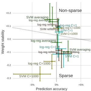
Prediction power – stability tradeoff. The choice of de-coder with the best predictive performance might not give the most stable weight maps, as seen by comparing figures 9 and10. Figure11shows the prediction–stability trade-off for different decoders and different parameter-tuning strategies. Overall, SVM and logistic-regression perform similarly and the dominant effect is that of the regular-ization: non-sparse, `2-penalized, models are much more

stable than sparse, `1-penalized, models. For non-sparse

models, averaging stands out as giving a large gain in sta-bility albeit with a decrease of a couple of percent in pre-diction accuracy compared to using C = 1 or C = 1000, which gives good prediction and stability (figures 9 and 11). With sparse models, averaging offers a slight edge for stability and, for SVM performs also well in prediction. C = 1000 achieves low stability (figure10), low prediction power (figure9), and a poor tradeoff.

Appendix D.2shows trends on datasets where the pre-diction is easy or not. For non-sparse models, averaging brings a larger gain in stability when prediction accuracy is large. Conversely, for sparse models, it is more beneficial to average in case of poor prediction accuracy.

Note that these experimental results are for common neuroimaging settings, with variance-normalization and univariate feature screening.

10-4₁₀-3₁₀-2₁₀-1₁₀0₁₀1₁₀2₁₀3₁₀4

Parameter tuning: C

50 60 70 80 90 100

Prediction accuracy

Accuracy

Nested cross validation

Validation set

SVM `2 10-4₁₀-3₁₀-2₁₀-1₁₀0₁₀1₁₀2₁₀3₁₀4

Parameter tuning: C

Log-reg `2 10-4₁₀-3₁₀-2₁₀-1₁₀0₁₀1₁₀2₁₀3₁₀4

Parameter tuning: C

SVM `1 10-4₁₀-3₁₀-2₁₀-1₁₀0₁₀1₁₀2₁₀3₁₀4

Parameter tuning: C

Log-reg `1

Figure 8: Tuning curves for SVM `2, logistic regression `2, SVM `1, and logistic regression `1, on the scissors / scramble discrimination for the Haxby dataset [19]. The thin colored lines are test scores for each of the internal cross-validation folds, the thick black line is the average of these test scores on all folds, and the thick dashed line is the score on left-out validation data. The vertical dashed line is the parameter selected on the inner cross-validation score.

4. Discussion and conclusion: lessons learned

Decoding seeks to establish a predictive link between brain images and behavioral or phenotypical variables. Prediction is intrinsically a notion related to new data, and therefore it is hard to measure. Cross-validation is the tool of choice to assess performance of a decoder and

CV +  averaging CV + refittingC=1 C=1000 ­8% ­4% ­2% 0% +2% +4% +8% Impact on prediction accuracy SVM log­reg Non-sparse models CV +  averaging CV + refittingC=1 C=1000 ­8% ­4% ­2% 0% +2% +4% +8% Impact on prediction accuracy SVM_log­reg Sparse models

Figure 9: Prediction accuracy: impact of the

parameter-tuning strategy. For each strategy, difference to the mean pre-diction accuracy in a given validation split.

CV +  averaging CV + refitting C=1 C=1000 ­0.3 ­0.2 ­0.1 0.0 +0.1 +0.2 +0.3 Impact on weight stability _SVM log­reg Non-sparse models CV +  averaging CV + refitting C=1 C=1000 ­0.3 ­0.2 ­0.1 0.0 +0.1 +0.2 +0.3 Impact on weight stability _SVM log­reg Sparse models

Figure 10: Stability of the weights: impact of the parameter-tuning strategy: for each strategy, difference to the mean stability of the model weights, where the stability is the correlation of the weights across validation splits. As the stability is a correlation, the unit is a different between correlation values. The reference is the mean stability across all models for a given prediction task.

to tune its parameters. The strength of cross-validation is that it relies on few assumptions and probes directly the ability to predict, unlike other model-selection procedures –eg based on information theoretic or Bayesian criteria. However, it is limited by the small sample sizes typically available in neuroimaging12.

An imprecise assessment of prediction. The imprecision on the estimation of decoder performance by cross-validation is often underestimated. Empirical confidence intervals of cross-validated accuracy measures typically ex-tend more than 10 points up and down (figure 5 and 6). Experiments on MRI (anatomical and functional), MEG, and simulations consistently exhibit these large error bars due to data scarcity. Such limitations should be kept in

12_{There is a trend in inter-subject analysis to acquire databases} with a larger number of subjects, eg ADNI, HCP. Conclusions of our empirical study might not readily transfer to these settings.

­5% 0% +5%

Prediction accuracy

­0.3 ­0.2 ­0.1 0.0 +0.1 +0.2

Weight stability

SVM averaging SVM C=1000 SVM C=1 SVM refitting SVM averaging SVM C=1000 SVM C=1 SVM refitting log­reg averaging log­reg C=1000 log­reg C=1 log­reg refitting log­reg averaging log­reg C=1000 log­reg C=1 log­reg refitting

Non­sparse

Sparse

Figure 11: Prediction – stability tradeoff The figure summarize figures9 and 10, reporting the stability of the weights, relative to the split’s average, as a function of the delta in prediction accuracy. It provides an overall summary, with errors bar giving the first and last quartiles (more detailed figures inAppendix D)

mind for many MVPA practices that use predictive power as a form of hypothesis testing –eg searchlight [28] or test-ing for generalization [26]– and it is recommended to use permutation to define the null hypothesis [28]. In addition, in the light of cross-validation variance, methods publica-tions should use several datasets to validate a new model. Guidelines on cross-validation. Leave-one-out cross-validation should be avoided, as it yields more variable results. Leaving out blocks of correlated observations, rather than individual observations, is crucial for non-biased estimates. Relying on repeated random splits with 20% of the data enables better estimates with less computation by increasing the number of cross-validations without shrinking the size of the test set.

Parameter tuning. Selecting optimal parameters can im-prove prediction and change drastically the aspects of weight maps (Fig.4).

However, our empirical study shows that for variance-normalized neuroimaging data, non-sparse decoders (`2

-penalized) are only weakly sensitive to the choice of their parameter, particularly for the SVM. As a result, rely-ing on the default value of the parameter often outper-forms parameter tuning by nested cross-validation. Yet, such parameter tuning tends to improve the stability of the maps. For sparse decoders (`1-penalized), default

pa-rameters also give good prediction performance. However, parameter tuning with model averaging increases stability and can lead to better prediction. Note that it is often useful to variance normalize the data (seeAppendix C). Concluding remarks. Evaluating a decoder is hard. Cross-validation should not be considered as a silver bullet. Nei-ther should prediction performance be the only metric. To assess decoding accuracy, best practice is to use repeated learning-testing with 20% of the data left out, while keep-ing in mind the large variance of the procedure. Any parameter tuning should be performed in nested cross-validation, to limit optimistic biases. Given the variance that arises from small samples, the choice of decoders and their parameters should be guided by several datasets.

Our extensive empirical validation (31 decoding tasks, with 8 datasets and almost 1 000 validation splits with nested cross-validation) shows that sparse models, in par-ticular `1 SVM with model averaging, give better

predic-tion but worst weight-maps stability than non-sparse clas-sifiers. If stability of weight maps is important, non-sparse SVM with C = 1 appears to be a good choice. Further work calls for empirical studies of decoder performance with more datasets, to reveal factors of the dataset that could guide better the choice of a decoder for a given task.

Acknowledgments

This work was supported by the EU FP7/2007-2013 under grant agreement no. 604102 (HBP). Computing re-source were provided by the NiConnect project

(ANR-11-BINF-0004 NiConnect) and an Amazon Webservices Re-search Grant. The authors would like to thank the devel-opers of nilearn13_{, scikit-learn}14 _{and MNE-Python}15 _for continuous efforts in producing high-quality tools crucial for this work.

In addition, we acknowledge useful feedback from Russ Poldrack on the manuscript.

References

[1] A. Abraham, F. Pedregosa, M. Eickenberg, P. Gervais, A. Mueller, J. Kossaifi, A. Gramfort, B. Thirion, G. Varoquaux, Machine learning for neuroimaging with scikit-learn, Frontiers in neuroinformatics 8 (2014).

[2] S. Arlot, A. Celisse, A survey of cross-validation procedures for model selection, Statistics surveys 4 (2010) 40.

[3] J. Ashburner, K.J. Friston, Diffeomorphic registration using geodesic shooting and gauss–newton optimisation, NeuroImage 55 (2011) 954–967.

[4] L. Breiman, Bagging predictors, Machine learning 24 (1996) 123.

[5] L. Breiman, P. Spector, Submodel selection and evaluation in regression. the x-random case, International statistical re-view/revue internationale de Statistique (1992) 291–319. [6] M.K. Carroll, G.A. Cecchi, I. Rish, R. Garg, A.R. Rao,

Pre-diction and interpretation of distributed neural activity with sparse models, NeuroImage 44 (2009) 112.

[7] X. Chen, F. Pereira, W. Lee, et al., Exploring predictive and reproducible modeling with the single-subject FIAC dataset, Hum. Brain Mapp. 27 (2006) 452.

[8] N.W. Churchill, G. Yourganov, S.C. Strother, Comparing within-subject classification and regularization methods in fMRI for large and small sample sizes, Human brain mapping 35 (2014) 4499.

[9] O. Demirci, V.P. Clark, V.A. Magnotta, N.C. Andreasen, J. Lauriello, K.A. Kiehl, G.D. Pearlson, V.D. Calhoun, A re-view of challenges in the use of fMRI for disease classifica-tion/characterization and a projection pursuit application from a multi-site fMRI schizophrenia study, Brain imaging and be-havior 2 (2008) 207–226.

[10] K.J. Duncan, C. Pattamadilok, I. Knierim, J.T. Devlin, Con-sistency and variability in functional localisers, Neuroimage 46 (2009) 1018.

[11] C.H. Fu, J. Mourao-Miranda, S.G. Costafreda, A. Khanna, A.F. Marquand, S.C. Williams, M.J. Brammer, Pattern classification of sad facial processing: toward the development of neurobio-logical markers in depression, Bioneurobio-logical psychiatry 63 (2008) 656–662.

[12] K. Gorgolewski, C.D. Burns, C. Madison, D. Clark, Y.O. Halchenko, M.L. Waskom, S.S. Ghosh, Nipype: a flexible, lightweight and extensible neuroimaging data processing frame-work in python., Front Neuroinform 5 (2011) 13.

[13] A. Gramfort, M. Luessi, E. Larson, D.A. Engemann,

D. Strohmeier, C. Brodbeck, R. Goj, M. Jas, T. Brooks, L. Parkkonen, et al., MEG and EEG data analysis with MNE-Python (2013).

[14] A. Gramfort, M. Luessi, E. Larson, D.A. Engemann,

D. Strohmeier, C. Brodbeck, L. Parkkonen, M.S. H¨am¨al¨ainen, MNE software for processing MEG and EEG data, Neuroimage 86 (2014) 446–460.

[15] A. Gramfort, B. Thirion, G. Varoquaux, Identifying predictive regions from fMRI with TV-L1 prior, PRNI (2013) 17.

13_{https://github.com/nilearn/nilearn/graphs/contributors} 14 https://github.com/scikit-learn/scikit-learn/graphs/ contributors 15 https://github.com/mne-tools/mne-python/graphs/ contributors

[16] L. Grosenick, B. Klingenberg, K. Katovich, B. Knutson, J.E. Taylor, Interpretable whole-brain prediction analysis with graphnet, NeuroImage 72 (2013) 304.

[17] M. Hanke, Y.O. Halchenko, P.B. Sederberg, S.J. Hanson, J.V. Haxby, S. Pollmann, PyMVPA: A python toolbox for multi-variate pattern analysis of fmri data, Neuroinformatics 7 (2009) 37.

[18] T. Hastie, R. Tibshirani, J. Friedman, The elements of statisti-cal learning, Springer, 2009.

[19] J.V. Haxby, I.M. Gobbini, M.L. Furey, et al., Distributed and overlapping representations of faces and objects in ventral tem-poral cortex, Science 293 (2001) 2425.

[20] J.D. Haynes, A primer on pattern-based approaches to fMRI: Principles, pitfalls, and perspectives, Neuron 87 (2015) 257. [21] J.D. Haynes, G. Rees, Decoding mental states from brain

activ-ity in humans, Nat. Rev. Neurosci. 7 (2006) 523.

[22] R. Henson, T. Shallice, M. Gorno-Tempini, R. Dolan, Face rep-etition effects in implicit and explicit memory tests as measured by fMRI, Cerebral Cortex 12 (2002) 178.

[23] A. Hoyos-Idrobo, Y. Schwartz, G. Varoquaux, B. Thirion, Im-proving sparse recovery on structured images with bagged clus-tering, PRNI (2015).

[24] Y. Kamitani, F. Tong, Decoding the visual and subjective con-tents of the human brain, Nature neuroscience 8 (2005) 679. [25] F.I. Karahano˘glu, C. Caballero-Gaudes, F. Lazeyras, D. Van

De Ville, Total activation: fMRI deconvolution through spatio-temporal regularization, Neuroimage 73 (2013) 121.

[26] A. Knops, B. Thirion, E.M. Hubbard, V. Michel, S. Dehaene, Recruitment of an area involved in eye movements during men-tal arithmetic, Science 324 (2009) 1583.

[27] R. Kohavi, A study of cross-validation and bootstrap for accu-racy estimation and model selection, in: IJCAI, volume 14, p. 1137.

[28] N. Kriegeskorte, R. Goebel, P. Bandettini, Information-based functional brain mapping, Proceedings of the National Academy of Sciences of the United States of America 103 (2006) 3863. [29] L.I. Kuncheva, J.J. Rodr´ıguez, Classifier ensembles for fMRI

data analysis: an experiment, Magnetic resonance imaging 28 (2010) 583.

[30] S. LaConte, J. Anderson, S. Muley, J. Ashe, S. Frutiger, K. Rehm, L. Hansen, E. Yacoub, X. Hu, D. Rottenberg, The evaluation of preprocessing choices in single-subject bold fMRI using npairs performance metrics, NeuroImage 18 (2003) 10. [31] S. LaConte, S. Strother, V. Cherkassky, J. Anderson, X. Hu,

Support vector machines for temporal classification of block de-sign fMRI data, NeuroImage 26 (2005) 317–329.

[32] G. Langs, B.H. Menze, D. Lashkari, P. Golland, Detecting sta-ble distributed patterns of brain activation using gini contrast, NeuroImage 56 (2011) 497.

[33] L.J. Larson-Prior, R. Oostenveld, S. Della Penna, G. Michalar-eas, F. Prior, A. Babajani-Feremi, J.M. Schoffelen, L. Marzetti, F. de Pasquale, F. Di Pompeo, et al., Adding dynamics to the human connectome project with MEG, Neuroimage 80 (2013) 190–201.

[34] D.S. Marcus, T.H. Wang, J. Parker, et al., Open access series of imaging studies (OASIS): cross-sectional MRI data in young, middle aged, nondemented, and demented older adults., J Cogn Neurosci 19 (2007) 1498.

[35] N. Meinshausen, P. B¨uhlmann, Stability selection, J Roy Stat Soc B 72 (2010) 417.

[36] V. Michel, A. Gramfort, G. Varoquaux, E. Eger, B. Thirion, Total variation regularization for fMRI-based prediction of be-havior, Medical Imaging, IEEE Transactions on 30 (2011) 1328. [37] K.J. Millman, M. Brett, Analysis of functional magnetic reso-nance imaging in python, Computing in Science & Engineering 9 (2007) 52–55.

[38] T.M. Mitchell, S.V. Shinkareva, A. Carlson, K.M. Chang, V.L. Malave, R.A. Mason, M.A. Just, Predicting human brain activ-ity associated with the meanings of nouns, science 320 (2008) 1191.

[39] J.M. Moran, E. Jolly, J.P. Mitchell, Social-cognitive deficits in

normal aging, J. Neurosci 32 (2012) 5553.

[40] J. Mouro-Miranda, A.L. Bokde, C. Born, H. Hampel, M. Stet-ter, Classifying brain states and determining the discriminating activation patterns: Support vector machine on functional MRI data, NeuroImage 28 (2005) 980.

[41] T. Naselaris, K.N. Kay, S. Nishimoto, J.L. Gallant, Encoding and decoding in fMRI, Neuroimage 56 (2011) 400.

[42] K.A. Norman, S.M. Polyn, G.J. Detre, J.V. Haxby, Beyond mind-reading: multi-voxel pattern analysis of fMRI data, Trends in cognitive sciences 10 (2006) 424.

[43] F. Pedregosa, G. Varoquaux, A. Gramfort, et al., Scikit-learn: Machine learning in Python, Journal of Machine Learning Re-search 12 (2011) 2825.

[44] W.D. Penny, K.J. Friston, J.T. Ashburner, S.J. Kiebel, T.E. Nichols, Statistical Parametric Mapping: The Analysis of Func-tional Brain Images, Academic Press, London, 2007.

[45] F. Pereira, T. Mitchell, M. Botvinick, Machine learning classi-fiers and fMRI: a tutorial overview, Neuroimage 45 (2009) S199. [46] J. Platt, Probabilistic outputs for support vector machines and comparisons to regularized likelihood methods, Advances in large margin classifiers 10 (1999) 61.

[47] R.A. Poldrack, D.M. Barch, J.P. Mitchell, et al., Toward open sharing of task-based fMRI data: the OpenfMRI project, Fron-tiers in neuroinformatics 7 (2013).

[48] R.A. Poldrack, Y.O. Halchenko, S.J. Hanson, Decoding the large-scale structure of brain function by classifying mental states across individuals, Psychological Science 20 (2009) 1364. [49] P.R. Raamana, M.W. Weiner, L. Wang, M.F. Beg, Thickness network features for prognostic applications in dementia, Neu-robiology of Aging 36, Supplement 1 (2015) S91 – S102. [50] P.M. Rasmussen, L.K. Hansen, K.H. Madsen, N.W. Churchill,

S.C. Strother, Model sparsity and brain pattern interpretation of classification models in neuroimaging, Pattern Recognition 45 (2012) 2085–2100.

[51] J.M. Rondina, J. Shawe-Taylor, J. Mour˜ao-Miranda, Stability-based multivariate mapping using scors, PRNI (2013) 198. [52] S. Ryali, K. Supekar, D. Abrams, V. Menon, Sparse logistic

re-gression for whole-brain classification of fMRI data, NeuroImage 51 (2010) 752.

[53] Y. Schwartz, B. Thirion, G. Varoquaux, Mapping cognitive on-tologies to and from the brain, NIPS (2013).

[54] J.D. Sitt, J.R. King, I. El Karoui, B. Rohaut, F. Faugeras, A. Gramfort, L. Cohen, M. Sigman, S. Dehaene, L. Naccache, Large scale screening of neural signatures of consciousness in patients in a vegetative or minimally conscious state, Brain 137 (2014) 2258–2270.

[55] S.C. Strother, J. Anderson, L.K. Hansen, U. Kjems, R. Kustra, J. Sidtis, S. Frutiger, S. Muley, S. LaConte, D. Rottenberg, The quantitative evaluation of functional neuroimaging experiments: the npairs data analysis framework, NeuroImage 15 (2002) 747. [56] S.C. Strother, P.M. Rasmussen, N.W. Churchill, L.K. Hansen, Stability and reproducibility in fMRI analysis, Practical Appli-cations of Sparse Modeling (2014) 99.

[57] G. Varoquaux, A. Gramfort, B. Thirion, Small-sample brain mapping: sparse recovery on spatially correlated designs with randomization and clustering, ICML (2012) 1375.

[58] G. Varoquaux, B. Thirion, How machine learning is shaping cognitive neuroimaging, GigaScience 3 (2014) 28.

[59] T.D. Wager, M.L. Davidson, B.L. Hughes, et al., Neural mech-anisms of emotion regulation: evidence for two independent prefrontal-subcortical pathways, Neuron 59 (2008) 1037. [60] O. Yamashita, M. aki Sato, T. Yoshioka, F. Tong, Y. Kamitani,

Sparse estimation automatically selects voxels relevant for the decoding of fMRI activity patterns, NeuroImage 42 (2008) 1414. [61] T. Yarkoni, J. Westfall, Choosing prediction over explanation in psychology: Lessons from machine learning, figshare preprint (2016).

X

1

X

2

X

1

X

2

Low separability High separability

time

X

1

time

X

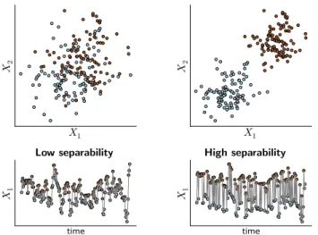
1

Figure A1: Simulated data for different levels of separability between the two classes (red and blue circles). Here, to simplify visualization, the data are generated in 2D (2 features), unlike the actual experiments, which are performed on 100 features. Top: The feature space. Bottom: Time series of the first feature. Note that the noise is correlated timewise, hence successive data points show similar shifts.

Appendix A. Experiments on simulated data

Appendix A.1. Dataset simulation

We generate data with samples from two classes, each de-scribed by a Gaussian of identity covariance in 100 dimensions. The classes are centered respectively on vectors (µ, . . . , µ) and (−µ, . . . , −µ) where µ is a parameter adjusted to control the separability of the classes. With larger µ the expected pre-dictive accuracy would be higher. In addition, to mimic the time dependence in neuroimaging data we apply a Gaussian smoothing filter in the sample direction on the noise (σ = 2). Code to reproduce the simulations can be found on https: //github.com/GaelVaroquaux/cross_val_experiments.

We produce different datasets with predefined separability by varying16 µ in (.05, .1, .2). FigureA1 shows two of these configurations.

Appendix A.2. Experiments: error varying separability Unlike with a brain imaging datasets, simulations open the door to measuring the actual prediction performance of a classi-fier, and therefore comparing it to the cross-validation measure. For this purpose, we generate a pseudo-experimental data with 200 train samples, and a separate very large test set, with 10 000 samples. The train samples correspond to the data avail-able during a neuroimaging experiment, and we perform cross-validation on these. We apply the decoder on the test set. The large number of test samples provides a good measure of predic-tion power of the decoder [2]. We use the same decoders as for brain-imaging data and repeat the whole procedure 100 times. For cross-validation strategies that rely on sample blocks –as with sessions–, we divide the data in 10 continuous blocks.

16_{the values we explore for µ were chosen empirically to vary} clas-sification accuracy from 60% to 90%.

Cross-validation Accuracy measured by cross-validation strategy for different separability

94.0% sep=0.2 77.2% sep=0.1 62.9% sep=0.05 Leave one sample out Leave one block out 20% left­out,   3 splits 20% left­out,   10 splits 20% left­out,   50 splits 86% 97% 94% 99% 98% 100% 57% 72% 67% 87% 83% 99% 55% 76% 66% 89% 81% 100% 57% 73% 68% 87% 84% 99% 58% 71% 69% 86% 84% 98% assymptotic prediction accuracy Separability 0.05 0.1 0.2

Figure A2: Cross-validation measures on simulations. Predic-tion accuracy, as measured by cross-validaPredic-tion (box plots) and on a very large test set (vertical lines) for different separability on the simulated data and for different cross-validation strategies: leave one sample out, leave one block of samples out (where the block is the natural unit of the experiment: subject or session), or random splits leaving out 20% of the blocks as test data, with 3, 10, or 50 random splits. The box gives the quartiles, while the whiskers give the 5 and 95 percentiles. Note that here leave-one-block-out is similar of 10 splits of 10% of the data.

Results. FigureA2 summarizes the cross-validation measures for different values of separability. Beyond the effect of the cross-validation strategy observed on other figures, the effect of the separability, ie the true prediction accuracy is also vis-ible. Setting aside the leave-one-sample-out cross-validation strategy, which is strongly biased by the correlations across the samples, we see that all strategies tend to be biased positively for low accuracy and negatively for high accuracy. This obser-vation is in accordance with trends observed on figure5.

Appendix B. Comparing parameter-tuning

strate-gies

FigureA3shows pairwise comparisons of parameter-tuning strategies, in sparse and non-sparse situations, for the best-performing options. In particular, it investigates when differ-ent strategies should be preferred. The trends are small. Yet, it appears that for low predictive power, setting C=1 in non-sparse models is preferable to cross-validation while for high predictive power, cross-validation is as efficient. This is con-sistent with results in figure5showing that cross-validation is more reliable to measure prediction error in situations with a good accuracy than in situations with a poor accuracy. Similar trends can be found when comparing to C=1000. For sparse models, model averaging can be preferable to refitting. We however find that for low prediction accuracy it is favorable to use C=1, in particular for logistic regression.

50% 60% 70% 80% 90% 100% Accuracy for cross­val + refitting 50% 60% 70% 80% 90% 100% Accuracy with C=1 SVM log­reg 50% 60% 70% 80% 90% 100% Accuracy for cross­val + refitting 50% 60% 70% 80% 90% 100% Accuracy with C=1000 _SVM log­reg Non-sparse models 50% 60% 70% 80% 90% 100% Accuracy for cross­val + averaging 50% 60% 70% 80% 90% 100% Accuracy with C=1 SVM log­reg 50% 60% 70% 80% 90% 100% Accuracy for cross­val + averaging 50% 60% 70% 80% 90% 100% Accuracy for cross­val + refitting SVM log­reg Sparse models

Figure A3: Comparing parameter-tuning strategies on pre-diction accuracy. Relating pairs of tuning strategies. Each dot corresponds to a given dataset, task, and validation split. The line is an indication of the tendency, using a lowess non-parametric local regression. The top row summarizes results for non-sparse models, SVM `2and logistic regression `2; while the bottom row gives results for sparse models, SVM `1and logistic regression `1.

Note these figures show points related to different studies and classification tasks. The trends observed are fairly homoge-neous and there are not regions of the diagram that stand out. Hence, the various conclusions on the comparison of decoding strategies are driven by all studies.

Appendix C. Results

without

variance-normalization

Results without variance normalization of the voxels are given in figure A4 for the correspondence between error mea-sured in the inner cross-validation loop, figureA5for the effect of the choice of a parameter-tuning strategy on the prediction performance, and figureA6for the effect on the stability of the weights.

Cross-validation on non variance-normalized neuroimaging data is not more reliable than on variance-normalized data (fig-ureA4). However, parameter tuning by nested cross-validation is more important than on variance-normalized data for good prediction (figureA5). This difference can be explained by the fact that variance normalizing makes dataset more comparable to each others, and thus a default value of parameters is more likely to work well.

In conclusion, variance normalizing the data can be impor-tant, in particular with non-sparse SVM.

50.0% 60.0% 70.0% 80.0% 90.0% 100.0%

Decoder accuracy on validation set 

50.0% 60.0% 70.0% 80.0% 90.0% 100.0%

Decoder accuracy 

measured by cross­validation

Intra subject Inter subject

Figure A4: Prediction error: cross-validated versus valida-tion set. Each point is a measure of predictor error measure in the inner cross-validation loop, or in the left-out validation dataset for a model refit using the best parameters. The line is an indication of the tendency, using a lowess non-parametric local regression.

CV +  averaging CV + refittingC=1 C=1000 ­8% ­4% ­2% 0% +2% +4% +8% Impact on prediction accuracy SVM log­reg Non-sparse models CV +  averaging CV + refittingC=1 C=1000 ­8% ­4% ­2% 0% +2% +4% +8% Impact on prediction accuracy SVM_log­reg Sparse models

Figure A5: Impact of the parameter-tuning strategy on the prediction accuracy without feature standardization: for each strategy, difference to the mean stability of the model weights across validation splits.

CV +  averaging CV + refitting C=1 C=1000 ­0.3 ­0.2 ­0.1 0.0 +0.1 +0.2 +0.3 Impact on weight stability _SVM log­reg Non-sparse models CV +  averaging CV + refitting C=1 C=1000 ­0.3 ­0.2 ­0.1 0.0 +0.1 +0.2 +0.3 Impact on weight stability _SVM log­reg Sparse models

Figure A6: Impact of the parameter-tuning strategy on sta-bility of weights without feature standardization: for each strategy, difference to the mean stability of the model weights across validation splits.

Figure A7: Prediction – stabil-ity tradeoff This figures gives the data points behind11, report-ing the stability of the weights, relative to the split’s average, as a function of the delta in predic-tion accuracy. Each point is cor-responds to a specific prediction task in our study.

­10% ­5% 0% +5%

Prediction accuracy

­0.3 ­0.4 ­0.2 ­0.1 0.0 +0.1 +0.2 +0.3 +0.4

Weight stability

SVM; C=1 SVM; C=1000 SVM; CV         + refitting SVM; CV      + averaging log­reg; C=1 log­reg; C=1000 log­reg; CV         + refitting log­reg; CV      + averaging Non-sparse models ­10% ­5% 0% +5%

Prediction accuracy

­0.3 ­0.4 ­0.2 ­0.1 0.0 +0.1 +0.2 +0.3 +0.4

Weight stability

Sparse models

Appendix D. Stability–prediction trends

Appendix D.1. Details on stability–prediction results Figure11summarizes the effects of the decoding strategy on the prediction – stability tradeoff. On figure A7, we give the data points that underly this summary.

Appendix D.2. Prediction and stability interactions

Figure 11 captures the effects of the decoding strategy across all datasets. However, some classification tasks are easier or more stable than others.

We give an additional figure, figureA8, showing this inter-action between classification performance and the best decod-ing strategy in terms of weight stability. The main factor of variation of the prediction accuracy is the choice of dataset, ie the difficulty of the prediction task.

Here again, we see that the most important choice is that of the penalty: logistic regression and SVM have overall the same behavior. In terms of stability of the weights, higher prediction accuracy does correspond to more stability, except for overly-penalized sparse model (C=1000). For non-sparse models, model averaging after cross-validation is particularly beneficial in good prediction situations.

Appendix E. Details on datasets used

Table A1 lists all the studies used in our experiments, as well as the specific prediction tasks. In the Haxby dataset [19] we use various pairs of visual stimuli, with differing difficulty. We excluded pairs for which decoding was unsuccessful, such as scissors versus bottle).

Appendix F. Details on preprocessing

Appendix F.1. fMRI data

Intra-subject prediction. For intra-subject prediction, we use the Haxby dataset [19] as provided from the PyMVPA [17] web-site –http://dev.pymvpa.org/datadb/haxby2001.html. De-tails of the preprocessing are not given in the original paper, beyond the fact that no spatial smoothing was performed. We have not performed additional preprocessing on top of this publicly-available dataset, aside from spatial smoothing with an isotropic Gaussian kernel, FWHM of 6 mm (nilearn 0.2, Python 2.7).

Inter-subject prediction. For inter-subject prediction, we use different datasets available on openfMRI [47]. For all the datasets, we performed standard preprocessing with SPM817: in the following order, slice-time correction, motion correction (realign), corregistration of mean EPI on subject’s T1 image, and normalization to template space with unified segmentation on the T1 image. The preprocessing pipeline was orchestrated through the Nipype processing infrastructure [12]. For each subject, we then performed session-level GLM with a design ac-cording to the individual studies, as described in the openfMRI files, using Nipy (version 0.3, Python version 2.7) [37]. Appendix F.2. Structural MR data

For prediction from structural MR data, we perform Voxel Based Morphometry (VBM) on the Oasis dataset [34]. We use SPM8 with the following steps: segmentation of the white matter/grey matter/CSF compartiments and estima-tion of the deformaestima-tion fields with DARTEL [3]. The puts for predictive models is the modulated grey-matter in-tensity. The corresponding maps can be downloaded with the dataset-downloading facilities of the nilearn software (function nilearn.datasets.fetch oasis vbm).

Appendix F.3. MEG data

The magneteoencephalography (MEG) data is from an N-back working-memory experiment made available by the Hu-man Connectome Project [33]. Data from 52 subjects and two runs was analyzed using a temporal window approach in which all magnetic fields sampled by the sensor array in a fixed time interval yield one variable set (see for example [54] for event re-lated potentials in electroencephalography). Here, each of the two runs served as validation set for the other run. For consis-tency, two-class decoding problems were considered, focussing on either the image content (faces VS tools) or the functional role in the working memory task (target VS low-level and high-level distractors). This yielded in total four classification anal-yses per subject. For each trial, the time window was then constrained to 50 millisecond before and 300 millisecond after event onset, emphasizing visual components.

17_{Wellcome Department of Cognitive Neurology,http://www.fil.} ion.ucl.ac.uk/spm

Figure A8: Prediction – sta-bility tradeoff The figure re-ports for each dataset and task the stability of the weights as a function of the prediction accu-racy measured on the validation set, with the different choices of decoders and parameter-tuning strategy. The line is an indi-cation of the tendency, using a lowess local regression. The sta-bility of the weights is the corre-lation across validation splits.

50.0% 60.0% 70.0% 80.0% 90.0%

Prediction accuracy

0.0 0.1 0.2 0.3 0.4 0.5 0.6 0.7 0.8

Weight stability

SVM l2 log­reg l2 SVM l1log­reg l1 All models 50.0% 60.0% 70.0% 80.0% 90.0%

Prediction accuracy

0.0 0.1 0.2 0.3 0.4 0.5 0.6 0.7 0.8

Weight stability

C=1 C=1000 CV + averagingCV + refitting Non-sparse models 50.0% 60.0% 70.0% 80.0% 90.0%

Prediction accuracy

0.0 0.1 0.2 0.3 0.4 0.5 0.6 0.7 0.8

Weight stability

C=1 C=1000 CV + averagingCV + refitting Sparse models # blocks (sess./subj.) mean accuracy

Dataset Description # samples Task SVM `2 SVM `1

bottle / scramble 75% 86% cat / bottle 62% 69% cat / chair 69% 80% cat / face 65% 72% cat / house 86% 95% cat / scramble 83% 92% chair / scramble 77% 91%

Haxby [19] fMRI 209 12 sess. chair / shoe 63% 70%

5 different subjects, face / house 88% 96%

leading to 5 experiments face / scissors 72% 83%

per task scissors / scramble 73% 87%

scissors / shoe 60% 64% shoe / bottle 62% 69% shoe / cat 72% 85% shoe / scramble 78% 88% consonant / scramble 92% 88% Duncan [10] fMRI, 196 49 subj. consonant / word 92% 89%

across subjects objects / consonant 90% 88%

objects / scramble 91% 88%

objects / words 74% 71%

words / scramble 91% 89%

fMRI negative cue / neutral cue 55% 55%

Wager [59] across subjects 390 34 subj. negative rating / neutral rating 54% 53%

negative stim / neutral stim 77% 73%

Cohen (ds009) fMRI 80 24 subj. successful / unsuccessful stop 67% 63%

across subjects

Moran [39] fMRI 138 36 subj. false picture / false belief 72% 71%

across subjects

Henson [22] fMRI 286 16 subj.

famous / scramble 77% 74%

across subjects famous / unfamiliar 54% 55%

scramble / unfamiliar 73% 70%

Knops [26] fMRI, 114 19 subj. right field / left field 79% 73%

across subjects

Oasis [34] VBM 403 52 subj. Gender discrimination 77% 75%

299 52 subj. faces / tools 81% 78%

HCP [33] MEG working memory 223 52 subj. target / non-target 58% 72%

across trials 135 52 subj. target / distractor 54% 53%

239 52 subj. distractor / non-target 55% 67%

Table A1: The different datasets and tasks. We report the prediction performance on the validation test for parameter tuning by 10 random splits followed by refitting using the best parameter.