Kinetic Shape Reconstruction

HAL Id: hal-02924409

https://hal.inria.fr/hal-02924409

Submitted on 2 Sep 2020

HAL is a multi-disciplinary open access

archive for the deposit and dissemination of

sci-entific research documents, whether they are

pub-lished or not. The documents may come from

teaching and research institutions in France or

abroad, or from public or private research centers.

L’archive ouverte pluridisciplinaire HAL, est

destinée au dépôt et à la diffusion de documents

scientifiques de niveau recherche, publiés ou non,

émanant des établissements d’enseignement et de

recherche français ou étrangers, des laboratoires

publics ou privés.

Jean-Philippe Bauchet, Florent Lafarge

To cite this version:

Jean-Philippe Bauchet, Florent Lafarge. Kinetic Shape Reconstruction. ACM Transactions on

Graph-ics, Association for Computing Machinery, 2020, �10.1145/3376918�. �hal-02924409�

JEAN-PHILIPPE BAUCHET and FLORENT LAFARGE,

manner is an enduring problem in Computer Graphics. Prior work, which typically operate by assembling planar shapes detected from input points, largely overlooked the scalability issue of processing a large number of shapes. As a result, they tend to produce overly simplified meshes with as-sembling approaches that can hardly digest more than one hundred shapes in practice. We propose a shape assembling mechanism which is at least one order magnitude more efficient, both in time and in number of processed shapes. Our key idea relies upon the design of a kinetic data structure for partitioning the space into convex polyhedra. Instead of slicing all the planar shapes exhaustively as prior methods, we create a partition where shapes grow at constant speed until colliding and forming polyhedra. This simple idea produces a lighter yet meaningful partition with a lower algorithmic complexity than an exhaustive partition. A watertight polygonal mesh is then extracted from the partition with a min-cut formulation. We demon-strate the robustness and efficacy of our algorithm on a variety of objects and scenes in terms of complexity, size and acquisition characteristics. In particular, we show the method can both faithfully represent piecewise planar structures and approximating freeform objects while offering high resilience to occlusions and missing data.

CCS Concepts: •Computing methodologies → Mesh models; Parametric

curve and surface models.

Additional Key Words and Phrases: Surface reconstruction, surface approxi-mation, polygonal surface mesh, kinetic framework

ACM Reference Format:

Jean-Philippe Bauchet and Florent Lafarge. 2020. Kinetic Shape

Recon-struction.ACM Trans. Graph. 39, 5, Article 1 (January 2020), 14 pages.

https://doi.org/10.1145/3376918

1 INTRODUCTION

Polygon meshes are the most widely used representations of sur-faces. They capture well the geometry of piecewise-planar objects, e.g. buildings, with ideally one facet for each planar component of an object. Polygonal meshes also approximate freeform shapes effec-tively [Botsch et al. 2010]. Although many mature algorithms exist to generatedense polygon meshes from data measurements such as Laser or MultiView Stereo (MVS) images [Berger et al. 2017], generating concise polygon meshes is still a scientific challenge. While user-guided Computer-Aided Design (CAD) enables the pro-duction of such quality meshes, ready for visualization, simulation or fabrication tasks, such interactive tools are labor-intensive and hence not suited to process large amounts of measurement data.

We consider the problem of converting unorganized 3D point clouds into surface polygon meshes with the following objectives:

Authors’ address: Jean-Philippe Bauchet; Florent Lafarge, Université Côte d’Azur, Inria, Sophia Antipolis, France, Firstname.Lastname@inria.fr.

Permission to make digital or hard copies of part or all of this work for personal or classroom use is granted without fee provided that copies are not made or distributed for profit or commercial advantage and that copies bear this notice and the full citation on the first page. Copyrights for third-party components of this work must be honored. For all other uses, contact the owner /author(s).

© 2020 Copyright held by the owner/author(s). 0730-0301/2020/1-ART1

https://doi.org/10.1145/3376918

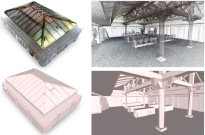
Fig. 1. Goal of our approach. Our algorithm converts a point cloud (top), here a 3M points laser scan, into a concise and watertight polygon mesh (bottom), in an automated manner. Planar components of the indoor scene (beams, walls, windows..) are captured by large facets whereas freeform objects (columns, tables...) are approximated by a low number of facets. Small objects (chairs, plants..) are filtered out. Model: Meeting Room.

• Fidelity. The output mesh must approximate well the input point cloud.

• Watertight. The output mesh is a watertight surface mesh free of self-intersections, bounding a 3D polyhedron. • Simplicity. The output mesh is composed of a small

num-ber of facets, ideally just-enough facets given a user-defined tolerance approximation error.

• Efficiency. The algorithm should be fast, scalable and proceed with a low memory consumption.

• Automation. The algorithm is fully automated, and takes only few intuitive user-defined parameters.

Existing methods or pipelines [Boulch et al. 2014; Mura et al. 2016; Nan and Wonka 2017] only partially fulfill the above objectives. They commonly operate by assemblingplanar shapes previously detected from the input points. Planar shapes are sets of inlier points to which a plane is fitted. They are used as intermediate representation between the input points and the output mesh. In most cases, the assembling of the planar shapes consists in slicing the 3D space bounding the input point cloud into a partition of convex polyhedral cells with the (infinite) supporting plane of each shape. The output mesh is then extracted by labeling the cells as inside or outside the input 3D objects. This approach yields concise polygon meshes, but is too compute- and memory-intensive to deal with complex objects and scenes. In our experiments this approach can only deal with scenes composed of less than 100 shapes, when executed on a standard desktop computer.

To achieve the above objectives, we propose a shape assembling method which is at least one order of magnitude more efficient than existing methods. Our primary contribution hinges on the design

and efficient implementation of akinetic data structure for parti-tioning the 3D space into convex polyhedra. Instead of slicing the 3D space by intersecting all supporting planes with each other, we generate a partition induced by convex planar polygons that grow at constant speed until colliding and creating polyhedra. Such a kinetic approach yields lighter yet meaningful 3D partitions with a significantly lower algorithmic complexity than the exhaustive partitioning. Our secondary contribution is a min-cut formulation for extracting the output surface mesh from the 3D partition. De-parting from prior work, our formulation relies upon a fast voting scheme that leverages the orientation of point normals. Finally, we evaluate and compare our approach with state-of-the-art methods against several quality and performance metrics, on a collection of 42 datasets that differ in terms of complexity, size and acquisition characteristics. This evaluation material will be released online. The goal of our method is illustrated in Figure 1.

2 RELATED WORK

Our review of previous work covers the detection of planar shapes from input points, the methods proceeding by assembling planar shapes, as well as alternative methods based on surface approxima-tion or geometry simplificaapproxima-tion.

Planar shape detection. Planar shape detection consists in cluster-ing the input point data into clusters of inlier points that lie near the same plane. Because we impose a minimal number of inliers for a planar shape, an input point is not necessarily associated to a shape. The common approaches operate by region growing [Marshall et al. 2001; Rabbani et al. 2006] or Ransac [Schnabel et al. 2007]. Region growing propagates a plane hypothesis to neighboring points until fitting conditions are no longer valid. Ransac proposes multiple plane hypotheses from some samples, verifies them against data, and selects the planes with the largest numbers of inliers. More ad-vanced approaches detect shapes and regularize them according to geometric relationships such as parallelism or orthogonality, either sequentially [Li et al. 2011; Oesau et al. 2016] or simultaneously [Monszpart et al. 2015]. Shapes can also be detected by learning approaches trained from CAD model databases [Fang et al. 2018; Li et al. 2019]. We refer to a recent survey for more details [Kaiser et al. 2018]. Our goal is different as we focus on assembling already detected planar shapes into a watertight polygonal mesh.

Shape assembling. Two main families of methods can be distin-guished to assemble planar shapes into a polygon mesh.

Connectivity methods analyze an adjacency graph between pla-nar shapes in order to extract the vertices, edges and facets of the output mesh [Chen and Chen 2008; Schindler et al. 2011; Van Krev-eld et al. 2011]. Although these methods are fast, they are likely to produce incomplete models on challenging data where adjacency graphs often contain linkage errors. One possible solution consists in completing the missing parts either interactively with user-guided mesh operations [Arikan et al. 2013], or automatically with dense triangle meshes [Holzmann et al. 2018; Lafarge and Alliez 2013]. Unfortunately, the first alternative does not offer a relevant solution for processing large volumes of data, and the second one does not output concise polygon meshes.

Slicing methods [Boulch et al. 2014; Chauve et al. 2010; Mura et al. 2016; Nan and Wonka 2017] are more robust to challenging data. They operate by slicing the input 3D space with the supporting planes of the detected shapes. The output partition is a decomposi-tion into convex polyhedral cells. The output mesh is then extracted by labeling the cells as inside or outside the surface, or equivalently, by selecting the polygonal facets of the cells that are part of the surface. The main limitation is the high algorithmic complexity for constructing the 3D partition, commonly performed via a binary space partition tree updated at each plane insertion [Murali and Funkhouser 1997]. Such a data structure can take hours to construct when more than 100 shapes are involved. Moreover, the returned partitions are overly complex, comprising many small anisotropic cells which are hampering the subsequent surface extraction pro-cess. Other approaches [Schnabel et al. 2009; Verdie et al. 2015] discretize the partitioning space instead of computing the exact geometry of the whole partition. This option is less costly, but often yields geometric artifacts when the discretization is not fine enough. In contrast, we do not slice all the shapes exhaustively, and instead grow them until colliding them with each other: this simple and natural idea yields lighter yet meaningful partitions with a lower algorithmic complexity.

Surface approximation. An alternative way to produce concise polygonal meshes is to first reconstruct a smooth surface from the input points and then simplify it. The first step can rely upon mature algorithms from the geometry processing toolbox such as the popu-lar Poisson reconstruction method [Kazhdan et al. 2006; Kazhdan and Hoppe 2013]. We refer to a recent survey that discusses the main algorithms for smooth surface reconstruction [Berger et al. 2017]. Once extracted, the dense triangle mesh is simplified into a coarser mesh. The most common approach consists in contracting edges until reaching a target number of facets [Garland and Heckbert 1997; Lindstrom 2000]. To better preserve the piecewise-planar structure of objects, the edge contraction operators can account for the planar shapes detected in the dense mesh [Salinas et al. 2015]. However, on planar parts such approaches yield triangle meshes whose adjacent facets are unlikely to be coplanar and form a meaningful decompo-sition. Other methods [Chen et al. 2013; Cohen-Steiner et al. 2004] alleviate this problem by connecting planar shapes using the adja-cency inferred from the input mesh. These surface approximation methods are in general effective, but they require as input a mesh that is both geometrically and topologically accurate to deliver faith-ful results. Unfortunately, such a requirement is rarely guaranteed from real-world data which are often highly corrupted by noise, outliers and occlusions.

Geometry simplification. Some work further reduce the combina-torial problem by imposing geometric assumptions for the output surface. For instance, the Manhattan-World assumption [Coughlan and Yuille 2000] enforces the generation of polycubes [Huang et al. 2014; Ikehata et al. 2015; Tarini et al. 2004] by imposing output facets to follow only three orthogonal directions. Another popular geometric assumption consists in constraining the output surface to specific disk-topologies. For instance, 2.5D view-dependent repre-sentations are typically well suited to buildings with airborne data

(a) (b) (c) (d)

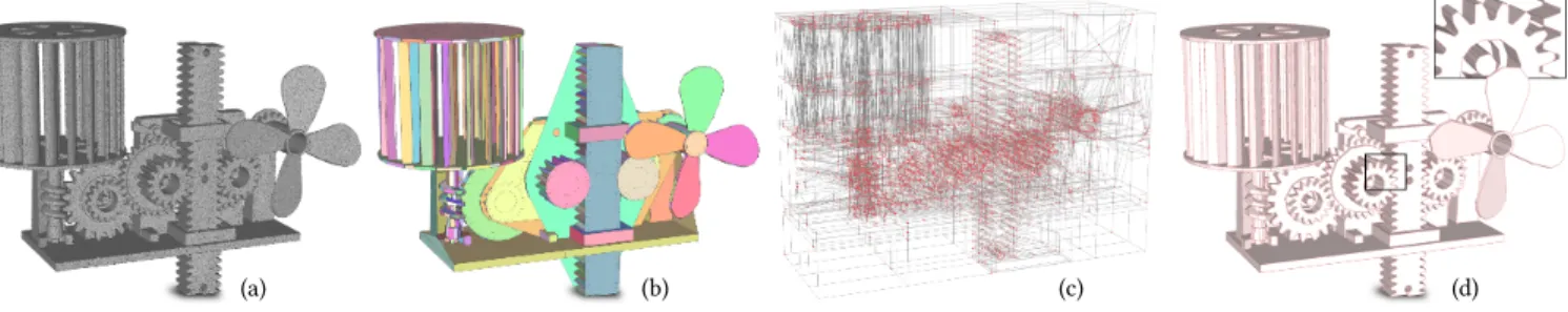
Fig. 2. Overview. Our algorithm takes as input a point cloud with oriented normals (a) and a configuration of convex polygons that approximate the object (b). Convex polygons are obtained through shape detection as the convex hulls of inlier points projected onto the shape. The 3D bounding box of the object is decomposed into polyhedra by kinetic partitioning from the convex polygons (c). The vertices and edges of polyhedra are displayed by red dots and grey line-segments respectively. A concise polygonal mesh is then extracted by labeling each polyhedron as inside or outside the object (d). Model: Full thing.

[Musialski et al. 2013] and facades with streetside images [Bodis-Szomoru et al. 2015]. Some approaches also approximate surfaces with specific layouts of polygonal facets. Such polyhedral patterns are particularly relevant for architectural design [Jiang et al. 2015, 2014]. Unfortunately such assumptions are only relevant for specific application domains. Beside piecewise-planar, our algorithm does not rely upon any geometric assumptions and remains generic.

3 OVERVIEW

Figure 2 illustrates the main steps of our method. Similarly to the popular Poisson algorithm [Kazhdan et al. 2006] and most of smooth surface reconstruction methods, our algorithm requires as input a point cloud with oriented normals. Point clouds are typically gen-erated from MVS, laser scanning or depth camera. Note that the oriented normals are commonly returned by these acquisition sys-tems: normals are estimated by principal component analysis or more advanced techniques whereas orientations are given by the point-to-camera center direction. Our algorithm also requires as input a configuration of planar shapes. The later is extracted from the point cloud by region growing [Rabbani et al. 2006] or Ransac [Schnabel et al. 2007] in our experiments. These algorithms are stan-dard geometric processing tools implemented in the CGAL library [Oesau et al. 2018]. More advanced methods exploiting filtering and regularization of planar shapes could be also considered. The shape extraction algorithms are typically controlled by two parameters: a fitting toleranceϵ that specifies the maximal distance of an inlier to its planar shape, and a minimal shape sizeσ that allows the rejection of planar shapes with a low number of inliers.

As a preliminary step, we compute the convex hull of each planar shape, i.e. the smallest convex polygon containing the projection of the inlier points on the optimal plane of the shape.

The first step of our method consists in partitioning the bounding box of the object into polyhedra, each facet of a polyhedron being a part or an extension of the convex polygons. This step relies on a kinetic framework in which convex polygons extend at constant speed until colliding with each other. When a collision between two or more polygons occurs, we modify the evolution of these polygons by either stopping their growth, changing their direction of propagation or splitting them. This set of polygons progressively

partitions the 3D space into polyhedra, the final partition being obtained when no polygon can grow anymore.

The second step extracts the polygonal surface mesh from the partition by labeling polyhedra as inside or outside the reconstructed object. We formulate it as a minimization problem solved by min-cut. Our objective function, called an energy, takes into account both the fidelity to input points and the simplicity of output models.

Our algorithm outputs a polygonal surface mesh whose facets lie on the supporting plane of the planar shapes. The output mesh is guaranteed to be watertight and intersection-free. Moreover, its volume is already decomposed into convex polyhedra, which is an interesting property for simulation tasks.

4 ALGORITHM 4.1 Kinetic partitioning

Background on Kinetic frameworks. Kinetic data structures have been introduced in Computational Geometry to track physical ob-jects in continuous motion [Guibas 2004; Guibas et al. 1983]. A kinetic data structure is composed of a set of geometricprimitives whose coordinates are continuous functions of time. The purpose of kinetic frameworks is to maintain the validity of a set of geo-metric properties on the primitives, also calledcertificates. When a certificate becomes invalid, geometric modifications are operated on the primitives to make the geometric properties valid again. This situation, also called anevent, happens, for instance, when several primitives collide. Kinetic frameworks show a strong algorithmic interest to dynamically order the times of occurrence of the events within apriority queue. A kinetic simulation then consists in un-stacking this queue until no primitive moves anymore. Kinetic data structures have been mostly designed for moving 2D primitives in the plane. Typical examples include dynamic 2D Delaunay triangu-lations with moving vertices [Agarwal et al. 2010], dynamic planar graphs with the propagation of line-segments [Bauchet and Lafarge 2018] or a pair of polygons in a motion [Basch et al. 2004]. To our knowledge, we are the first to design and implement a kinetic data structure that collides polygons in the 3D space.

Primitives and kinetic data structure. The primitives of our kinetic framework are polygons whose vertices move at constant speeds

along given directions. The initial set of polygons is defined as the convex hulls of the planar shapes. Polygons grow by uniform

t0+ δt

t0

scaling: each vertex moves in the op-posite direction to the center of mass of the initial polygon (see inset). The underlying kinetic data structureP is the set of these polygons that, we as-sume, do not intersect with each other. When two or more polygons intersect, we modify primitives to maintain valid

the intersection-free property. For generality reasons, polygons extend at constant speed: no planar shape is favored over others.

Certificates. For each primitivei, we define the certificate function Ci(t ) as Ci(t )= N Ö j=1 j,i Pri,j(t ) (1)

whereN is the number of primitives of the kinetic data structure, andPr_i,j(t ) the predicate function that returns 0 when primitive i collides with primitivej, i.e. when the minimal distance between the polygon boundary of primitivei and the closed polygon of primitive j equates zero for the first time, and 1 otherwise. Primitive i is called thesource primitive, andj, the target primitive. Because the directions of propagation of polygons can change along time, the computation of this minimal distance is a difficult task in practice. We detail in Section 5 how we compute this distance efficiently.

Initialization. Before starting growing the set of convex hulls, we first need to decompose them into intersection-free polygons. As illustrated in Figure 3, each non intersection-free polygon is cut along the intersection lines with the other polygons. Because the propagation of polygons outside the bounding box is not relevant in practice, we also insert the six facets of the bounding box into the kinetic data structure. We denote byP0this set of intersection-free

polygons. In addition, we populate the priority queue by computing and sorting in ascending order the times of collision, i.e. times for which certificatesC_i(t )= 0 for each polygon i of P0.

Fig. 3. Initialization. At t = 0, the blue polygon intersects two other poly-gons, the intersections being represented by the red and green line-segments (left). We decompose it into intersection-free polygons with cuts along the intersection lines (red and green dashed lines). The direction of propagation of original vertices (black points) are unchanged while the new vertices are either kept fixed when located at the junction of several intersection lines (white points) or are moving along the intersection lines (gray points). We denote them as frozen vertices and sliding vertices respectively (right). A polygon is active if not all its vertices are frozen.

Updating operations. When a collision between primitives occurs, we need to update the kinetic data structure to keep the set of polygons free of intersection.

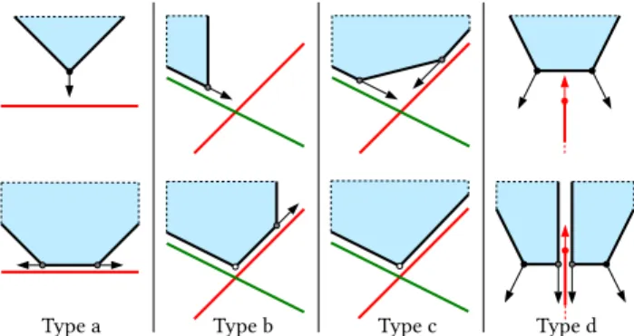
We first modify the source polygon. As illustrated in Figure 4, four collision types are distinguished:

• A vertex of the source polygon collides with the target poly-gon (type a). We replace the vertex by two sliding vertices that move along the intersection line in opposite directions. • A sliding vertex of the source polygon collides with the target polygon (type b). We modify the direction of propagation of the sliding vertex to follow the intersection line with the target polygon. We also create a frozen vertex where the intersection line with the target polygon and the intersection line with the polygon supporting the sliding vertex before collision meet.

• A sliding vertex of the source polygon collides with the target polygon while a sliding vertex guided by the target polygon already exists (type c). We create a frozen vertex where the two intersection lines meet: the propagation of the source polygon is locally stopped.

• An edge of the source polygon collides with an edge or vertex of the target polygon (type d). Source and target polygons are split along their intersection line with the creation of eight sliding vertices (two per new polygon).

These four collision types include all the possible cases of collisions between two polygons. In particular, collisions between two copla-nar polygons are processed in types a and b. Also, the collision between an edge of the source polygon and the interior of the target polygon is simply treated as type a.

Type a Type b Type c Type d

Fig. 4. Collision typology and corresponding primitive updates. A vertex or an edge of the source polygon (blue shape) typically collides with the target polygon (red segment) in four different manners (top). The corresponding updates consist in inserting sliding vertices and/or frozen vertices in the source polygon for types a, b and c, or splitting polygons for type d (bottom).

In many situations, it is interesting to extend the source polygon on the other side of the target polygon. To decide whether this should happen, we define acrossing condition which is valid if (i) the source polygon has collided a number of times lower than a user-specified parameterK, or else if (ii) relevant input points omitted during shape detection can be found in the other side of the target polygon. ParameterK is a trade-off between the complexity of the polyhedron partition and the robustness to missing data. In particular,K = 1 yields the simplest partition whereas K = ∞

produces the partition returned by the exhaustive plane slicing approach. ParameterK is typically set to 2 in our experiments. The second criterion is data-driven: it counts the number of input

ϵ d

points contained in a box (black dashed rectangle in the inset) located behind the target polygon (red segment) and aligned with the source polygon (black segment). In the inset, this number is

5. The thickness of the box is twice the fitting toleranceϵ used for detecting planar shapes while its depthd is chosen experimentally as 10 times the average distance bd between neighbors of the k-nearest neighbor graph of the input points. Assuming the average density of points sampling the object surface is approximately bd−2, we validate the criterion when the density of points in the box is higher than half of bd−2in practice. This data-driven criterion is useful to recover planar parts missed during shape detection, as shown in Figure 5.

Fig. 5. Data-driven criterion. Small planar parts are often missed during shape extraction (see missing shapes on the left closeup). The output surface then becomes overly simplified (middle). The data-driven criterion allows us to recover the correct geometry when these planar parts belong to a repetitive structure such as the ramparts (right). Model: Castle.

If the crossing condition is valid, a new polygon that extends the source primitive on the other side of the target polygon must be

type a type b

inserted into the kinetic data structure. This situation can only happen to collision types a and b in Figure 4. The new polygon is initialized as a trian-gle composed of two sliding

ver-tices and one original vertex for type a, or of two sliding verver-tices and one frozen vertex for type b (see inset).

Finally we update the priority queue. We first remove the pro-cessed event between the source and the target polygons from the queue. If the two polygons have been modified, we recompute their times of collision with the active polygons if not all their vertices are frozen, or remove their times of collision with the active polygons from the queue otherwise. If new polygons have been created (type d or types a/b with the crossing condition valid), we compute their times of collision with the active polygons and insert them into the priority queue.

Finalization. When the priority queue is empty, the kinetic data structure does not evolve anymore. The output polygons are com-posed of frozen vertices only and form a partition of polyhedra. We

extract this partition as a 3D combinatorial map [Damiand 2018]. The 2-cells of the combinatorial map correspond to the union of the internal facets, which are the final set of intersection-free polygons P, and the external facets located on the sides of the 3D bounding box. Polyhedra, or 3-cells of the combinatorial map, are then ex-tracted as the smallest closed sets of adjacent facets. Note that the polyhedra are convex by construction. The global mechanism of the kinetic partitioning is summarized in Algorithm 1. A detailed pseudo-code is also provided in supplementary material.

ALGORITHM 1: Kinetic partitioning

Initialize the kinetic data structureP to P0

Initialize the priority queueQ

whileQ , ∅ do

Pop the source and target primitives fromQ

Test the crossing condition of the source primitive

UpdateP

UpdateQ

end while

Finalize the tessellation

4.2 Surface extraction

We now wish to extract a surface from the partition of polyhedra. We operate a min-cut to find an inside-outside labeling of the polyhedra, the output surface being defined as the interface facets between

out out out in in out out

inside and outside (see the red polygon in the inset). Be-cause the kinetic partition is a valid polyhedral embedding, this strategy guarantees the out-put surface to be watertight (i.e.

composed of close surfaces) and intersection-free, similarly to min-cut formulations operating on 3D triangulation [Labatut et al. 2009]. Moreover, it provides a decomposition of the output model into

out in

in out convex polyhedra. The output surface mesh is however not guaranteed to be 2-manifold. As illustrated in the inset, two polyhedra labeled as inside can be connected along one edge or at one

vertex while being facet-adjacent to polyhedra all labeled as outside. The methods relying upon this approach [Boulch et al. 2014; Chauve et al. 2010; Verdie et al. 2015] typically assign an inside-outside guess on each polyhedron by ray shooting: this is both imprecise in presence of missing data and computationally costly. We instead propose a faster voting scheme that exploits the oriented normals of inlier points to more robustly assign a guess on a portion of the polyhedra only.

We denote byC, the set of polyhedra of the tessellation, and by xi = {in, out}, the binary label that specifies whether polyhedron i

is inside (x_i = in) or outside (x_i = out) the surface. We measure the quality of a possible output surfacex= (xi)_{i ∈C}with a two-term energy of the form

U (x)= D(x) + λV (x) (2) whereD(x) and V (x) are terms living in [0, 1] that measure data fidelity and surface complexity respectively.λ ∈ [0, 1] is a parameter

balancing the two terms. The optimal output surface that minimizes U is found by a max-flow algorithm [Boykov and Kolmogorov 2004]. Data fidelityD(x) measures the coherence between the inside-outside label of each polyhedron and the orientation of normals of inlier points. Similarly to signed distances proposed in smooth sur-face reconstruction, we assume here that the normals point towards the outside. After associating each inlier point with the facet of the partition that contains its orthogonal projection on the infinite plane of its planar shape, we express data fidelity by a voting on each inlier point under the form

D(x)= 1 |I | Õ i ∈C Õ p ∈Ii di(p, xi) (3)

where|I | is twice the total number of inlier points, Iiis the set of inlier points associated with all the facets of polyhedroni, and di(p, xi) is a voting function that tests whether the orientation of inlier pointp is coherent with the label x_i of polyhedroni.

p n®

® u

polyhedroni

polyhedronj

This function is defined byd_i(p, in)= 1_{{ ®n · ®u >0}} andd_i(p, out ) = 1_{{ ®n · ®u <0}} where 1_{{. }}is the characteristic func-tion,n the normal vector of inlier® pointp, and ®u the vector from p to the center of mass of polyhedroni. In the inset example, we prefer as-signing labelin to polyhedroni and labelout to polyhedronj. In particu-lar,d_i(p, x_i = out) and d_j(p, x_j = in)

return a penalty of 1 whereasd_i(p, x_i = in) = d_j(p, x_j = out) = 0. Because the voting functiondiis binary, normals only need to point towards the right half-space separating the facet. This brings ro-bustness to imprecise normal directions.

The second termV (x) is more conventional: it measures the com-plexity of the output surface by its area, where lower is simpler. It is expressed by V (x)= 1 A Õ i∼j aij· 1_{x i,xj} (4) wherei ∼ j denotes the pairs of adjacent polyhedra, a_ijrepresents the area of the common facet between polyhedrai and j, and A is a normalization factor defined as the sum of the areas of all facets of the partition. As shown in Figure 6, this term avoids the surface zigzagging. Giving a too high importance to this term however shrinks the surface. In our experiments, we typically setλ to 0.5.

5 IMPLEMENTATION DETAILS

Our algorithm has been implemented in C++ using the CGAL library. In particular, we used the exact predicates, exact constructions ker-nel for the computation of distances and times of collision. We now explain several important implementation details that improve the efficiency, stability and scalability of our method.

Reformulation as collaborative 2D collision problems. At each up-date of the kinetic data structure, the propagation of the source polygon is likely to be modified. Consequently, the update of the priority queue requires the distance of this polygon to each other active polygons to be recomputed. To avoid such time consuming

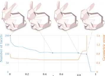
0 50 100 150 200 Numb er of facets 0 0.4 0.8 1.2 1.6 Ge ometric err or 0 0.2 0.4 0.6 0.8 1 λ

Fig. 6. Impact of parameter λ. Increasing λ simplifies the output surface by reducing the number of facets (blue curve). A too high value however makes object parts disappear and increases the geometric error (red curve). The best compromise between simplicity and accuracy is returned between 0.4 and 0.8. The geometric error is computed as the symmetric mean Hausdorff distance between input points and output mesh. Model: Stanford bunny.

operations, we algorithmically reformulate the 3D collision prob-lem as N collaborative propagations of polygons in 2D controlled by a global priority queue, N being the number of planar shapes. The intuition behind this reformulation is that two non-coplanar polygons cannot

col-lide somewhere else than along the 3D line intersecting their re-spective planes. This 3D line being repre-sented by a 2D line in

the planes containing the two polygons (see dashed-lines in the inset), we can then use a simple point-to-line distance in 2D to compute the times of collisions. Although more events must be processed with this reformulation, the update of the priority queue is drastically simplified.

Computation with rationals. Our implementation relies upon the exact predicates, exact constructions kernel of the CGAL library. All distances and times of collisions are computed with rational numbers, after converting the input planar primitives with decimal coordinates into rationals. The final kinetic partition is then guar-anteed to be a valid polyhedron embedding, and the output mesh to not contain degenerated facets. Note that, because the vertices of the kinetic partition are necessarily intersections of 3 initial sup-porting planes, the growth of the rational representation remains low. Once extracted by the min-cut formulation, the output mesh is exported with a double precision whose approximation error with the rational numbers is upper-bounded by a user-defined value (set to 10−12in our experiments using the Lazy_exact_nt CGAL num-ber type). In addition, the orientation of the input planar shapes is expressed to the nearest tenth of a degree so that the orientation of two non-coplanar shapes necessarily differs from at least 0.1 de-gree. These two ingredients are an efficient way to avoid potential

Poly. (Subdivs = 1) Poly. (Subdivs = 2) Poly. (Subdivs = 4) Poly. (Subdivs = 8) Poly. (Subdivs = 16)Subdivision by 16

Subdivision by 8 Subdivision by 4 Subdivision by 2 No subdivisions 10 102 103 104 0.1 1 10 102 103 104 Running time ( s.)

Number of planar shapes

Memor

y

p

eak

(MB)

Number of planar shapes

10 102 103 104

10 102 103 104

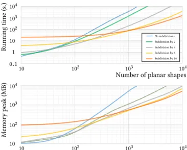
Fig. 7. Performances with spatial subdivision. The lowest curve in each graph indicates the most efficient subdivision scheme given the number of planar shapes. For instance, one thousand planar shapes can be processed in

one minute by subdividing the 3D bounding box into 83

blocks (yellow curve in top graph), whereas half an hour is required without subdivision (blue curve). Memory peak evolves similarly to running time. The performances have been obtained from 100k input points uniformly sampled on a sphere.

imprecision during the floating point conversion in practice: among all our runs, we never experimented imprecision cases leading to self-intersecting facets in the kinetic partition.

Priority queue. Although all possible collisions should be inserted into the priority queue, we observe that an active vertex often col-lides with only the three closest lines. To reduce memory consump-tion and processing time, we thus restrict the number of collisions per vertex in the priority queue to three. If the three collisions occur and the vertex is not frozen we insert the three next collisions of this vertex in the priority queue and repeat this operation as many times as necessary. This reduces running time and memory consumption by a factor close to 1.5 and 3 respectively.

Simultaneous collisions. Our implementation sequentially pro-cesses the collisions between pairs of primitives, and do not directly handle situations where three primitives or more mutually collide at the same time. We treat these particular situations by simply applying an infinitesimal perturbation on the initial coordinates of the polygon vertices while maintaining the vertices in the sup-porting planes. This simple trick avoids a laborious implementation of the numerous cases of simultaneous collisions between k primi-tives while preserving the efficiency of the algorithm. This technical choice is also based on the observation that such simultaneous mul-tiple collisions is improbable in practice when planar shapes are detected with a floating precision.

Spatial subdivision. To increase the scalability of our algorithm, we offer the option to subdivide the bounding box of the object into uniformly-sized 3D blocks in which independent kinetic parti-tionings are operated. For each block, we collect the closest planar

shapes, i.e. those whose initial convex polygon is either inside the block or intersecting at least one of its sides. We then operate the ki-netic partitioning inside the block from this subset of planar shapes. Once all blocks are processed, we merge the polyhedral partitions. An important speed-up factor lies into the fact that only a portion of planar shapes is involved in the partitioning of each block. Figure 7 plots the time and memory savings against the number of planar shapes for several subdivision schemes. While the savings are signif-icant, the use of spatial subdivision produces a simplified polyhedral partition as polygons do not propagate to neighboring blocks. This may affect the quality of the output surface with typically the pres-ence of extra facets at the borders of blocks. Figure 8 illustrates this compromise between algorithm efficiency and surface quality. Our implementation treats blocks sequentially, but one could process them in parallel for even better performances.

| F |=21K #f=314 t=260 m=0.57 | F |=18K #f=321 t=126 m=0.28 | F |=12K #f=375 t=30 m=0.19 no subdivision subdivision by 2 subdivision by 4

Fig. 8. Spatial subdivision: efficiency vs quality. Our algorithm produces an ideal mesh with 314 polygonal facets from 314 planar shapes approxi-mating a sphere (left). Subdividing the bounding box into blocks reduces running time and memory consumption, and produces simplified polyhedra partitions (top). This option may degrade the quality of the output meshes (bottom) with typically the presence of extra facets at the block borders (see closeup). |F |, #f, t and m correspond to the number of facets in the polyhedral partition, the number of polygonal facets in the output mesh, running time (in sec) and memory peak (in GB) respectively.

6 RESULTS

We evaluated our algorithm with respect to our fidelity, simplicity and efficiency objectives. We measure the fidelity to 3D data by the symmetric mean Hausdorff (SMH) distance between input point cloud and output mesh. The simplicity of output representation is quantified by the ratio between the number of output facets to the number of initial planar shapes. We measure the efficiency of the algorithm by both running time and memory peak. In addition to these four measures, we also evaluate the scalability of algorithms by the maximal number of planar shapes that can be processed without exceeding both 105seconds on a single computer with a core i9 processor clocked at 2.9Ghz, and 32GB memory consumption. Input planar shapes were extracted by the region growing implementation of the CGAL library [Oesau et al. 2018]. The fitting toleranceϵ were typically set to 0.2% of the bounding box diagonal on large scenes and 1% on more simple objects and multi-view stereo acquisitions. The minimal shape sizeσ ranged from 0.001% to 1% of the total number of input points, depending on the complexity of scenes.

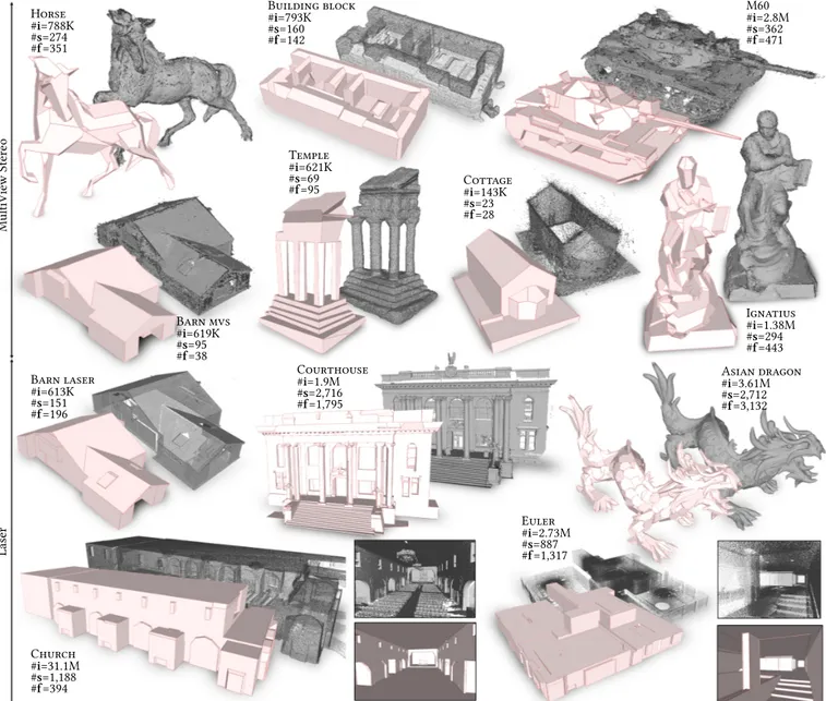
Laser MultiVie w Ster e o Ignatius #i=1.38M #s=294 #f=443 M60 #i=2.8M #s=362 #f=471 Temple #_i=621K #s=69 #f=95 Building block #i=793K #s=160 #f=142 Horse #i=788K #s=274 #f=351 Cottage #i=143K #s=23 #f=28 Barn mvs #i=619K #s=95 #f=38 Barn laser #i=613K #s=151 #f=196 Church #i=31.1M #s=1,188 #f=394 Euler #i=2.73M #s=887 #f=1,317 Courthouse #i=1.9M #s=2,716 #f=1,795 Asian dragon #i=3.61M #s=2,712 #f=3,132

Fig. 9. Reconstructions from various multi-view stereo and laser datasets. Our algorithm produces concise polygonal meshes for both freeform objects such as Horse, Ignatius and Asian dragon and piecewise-planar structures such as Church, Barn and Euler. Complex objects such as M60 are approximated with a good amout of details by a few hundred facet mesh only. Because of a more accurate detection of planar shapes, our algorithm typically performs better from laser datasets with more detailed reconstructed models (see Barn mvs and Barn laser models). #i, #s and #f correspond to the number of input points, planar shapes and output facets respectively.

The exact values are given in supplementary material for the 42 tested models. Globally speaking, this pair of values must be chosen according to the desired abstraction level where the higher the values ofϵ and σ , the more concise the output model. Note that the optimal choice for these two values can also be learned from training sets in which each point cloud is associated with a targeted configuration of planar shapes [Fang et al. 2018].

Flexibility. Our algorithm has been tested on a variety of ob-jects and scenes. Freeform obob-jects such as Stanford Bunny, Hand,

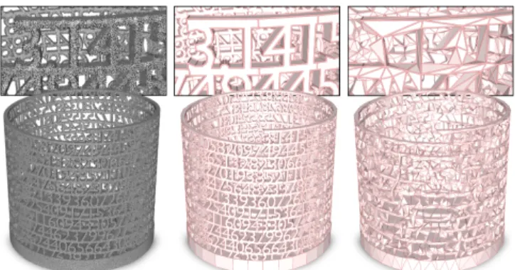
Horse or Ignatius are approximated by compact polygonal meshes. For instance, each digit of Tower of Pi is represented by only a few polygonal facets in Figure 10. Piecewise-planar structures such as Barn, Euler, Meeting room or Full thing are reconstructed with fine details as long as planar shapes are correctly detected from data. We also tested our algorithm on different acquisition systems. MultiView Stereo (MVS) datasets presented in Figure 9 have been generated by COLMAP [Schönberger and Frahm 2016] from image sequences mostly provided by the Tanks and Temples benchmark [Knapitsch et al. 2017]. Because of the high amount of

Fig. 10. Reconstruction of Tower of Pi. 10.8K planar shapes are detected from 2.9M input points (left) and assembled by our algorithm into a concise polygonal mesh of 12.1K facets (middle). Each digit is nicely represented by a few facets (see closeups). In contrast, the mesh produced by the tra-ditional approximation pipeline (Screened Poisson [Kazhdan and Hoppe 2013] then QEM edge collapse [Garland and Heckbert 1997]) at the same output complexity fails to preserve the structure of the digits (right).

noise, these point clouds are particularly challenging to reconstruct. Point clouds generated by Laser scanning are geometrically more accurate, but suffer from missing data and heterogeneous point density. As illustrated with Barn model, our algorithm typically returns more accurate output meshes with Laser acquisition. MVS point clouds are often too noisy to capture fine details with small planar shapes. Conversely, frequent occlusions contained in Laser scans are effectively handled by our kinetic approach that naturally fills in empty space in between planar shapes. Some point clouds have also been sampled from CAD models. This is the case of Full thing, Castle, Tower of Pi and Hilbert cube whose CAD models originate from the Thingi10k database [Zhou and Jacobson 2016].

0% noise 0.5% noise 1% noise 1.5% noise

Fig. 11. Robustness to noise. Our algorithm is robust to noise as long as planar shapes can be decently extracted from input points. At 1% noise, some shapes become missing or inaccurately detected, leading to an overly complex output mesh. At 1.5%, the poorly extracted shapes do not allow us to capture the structure of the cube anymore. Note that normals have been recomputed for each degraded point cloud. Model: Hilbert Cube.

Robustness to imperfect data. Figure 11 shows the robustness of our algorithm to noise. Below 1% noise (with respect to the bounding box diagonal), our algorithm outputs accurate meshes. Above 1%, planar shapes become missing or inaccurately detected. Because our goal is not to correct or complete the shape configuration, the output mesh cannot preserve the structure of the object anymore. Beside

noise, the propagation of planar shapes within the kinetic algorithm offers high resilience to occlusions, especially when parameterK is strictly greater than 1. This allows, for instance, to recover the skylights on Barn laser and the rampart structures on Castle. As illustrated in Figure 12, our algorithm is also robust to heterogeneous sampling and outliers by inheriting the good behavior of shape detection methods with respect to these two defects.

+500% outliers +1500%outliers −25% points −75% points

Fig. 12. Robustness to outliers and heterogeneous sampling. Our algorithm returns an accurate model when adding 500% of outliers in the object bound-ing box, but starts compactbound-ing the structure around 1500% of added outliers. In the two right examples, the point clouds have been progressively sub-sampled from the bottom left to the top right of the cube in a linear manner. Our algorithm is resilient to such heterogeneous sampling as long as shapes can be retrieved in the low density of points.

Performances. Table 1 presents the performances of our algorithm in terms of running time and memory consumption from various models. Timings and memory consumption of all the results pre-sented in the paper are provided in supplementary material. Kinetic partitioning is typically the most time-consuming step. In particular, around 90% of computing efforts focuses on the processing of the priority queue. The total number of collisions depends on multiple factors which include the number of initial convex polygons, their number of vertices, their mutual positioning within the bounding box as well as parameter K. For instance, 53K collisions are pro-cessed for the 75 shapes of the Hand model shown in Figure 16. The most frequent collision types are b and c with an occurrence of 51% and 30% respectively. Collision type a is the most time-consuming update because of the costly insertion of several sliding vertices in the kinetic data structure.

Meeting room Full thing T o wer of Pi Temple Church # input points 3.07M 1.38M 2.9M 621K 31.1M # planar shapes 1,655 1,648 10.8K 69 1,188 #output facets 1,491 1,807 12,059 95 394 Subdivision 4 4 8 no 2

kinetic partitioning (sec) 197 443 1,696 18 310

surface extraction (sec) 84 49 105 17 717

memory peak (MB) 642 552 3,864 69 325

Surface e xtraction Partitioning Kinetic (K = 1) Kinetic (K = 2) Exhaustive IP solver GC solver 103 102 10 1 0 50 100 150 200 250 Time (s.) Number of shapes 105 104 103 102 10 1 102 103 104 105 106 Time (s.) Number of polyhedra 1 10 102 103 104 105 0 50 100 150 200 250 Memory peak (MB.) Number of shapes 103 102 10 1 102 103 104 105 106 Memory peak (MB.) Number of polyhedra 1 10 102 103 104 105 0 50 100 150 200 250 Number of polyhedra Number of shapes 0.8 0.6 0.4 0.2 0 102 103 104 SMH error Number of polyhedra

Fig. 13. Performances of partitioning and surface extraction. Kinetic partitioning produces more compact sets of polyhedra in a more time- and memory-efficient manner than exhaustive partitioning (top row). The gain becomes significant from 150 planar shapes with one (respectively two) order of magnitude saving in memory consumption (resp. number of polyhedra). When partitions contain less than one thousand polyhedra, our graph-cut (GC) formulation for surface extraction and the integer programming (IP) solver of [Nan and Wonka 2017] have similar running times and geometric errors (bottom row). However, the IP solver consumes more memory and can hardly digest partitions with more than ten thousands polyhedra. Moreover, the IP solver is less stable as running times and memory peaks can unpredictably vary (see light orange bands in bottom left/middle graphs). In contrast, the variation in time observed for our GC formulation only depends on the number of input points, the lower (respectively upper) bound of the light blue band corresponding to the model with the lowest (resp. highest) number of points. Statistics were drawn from a collection of seven different models with input point sizes ranging from 100K to 5M.

The costly operation for the surface extraction step is the compu-tation of the voting functiondi(p, xi) which must be performed for each inlier point. The shape detection step, which is not a contri-bution of our work, typically requires few seconds for processing several millions input points. In terms of scalability, our algorithm can handle tens of thousands of planar shapes on a standard com-puter without parallelization schemes.

Ablation study. We evaluated the impact of the kinetic partition-ing and the surface extraction on the performances of our algorithm. First, we compared the performances of exhaustive and kinetic partitionings. The top graphs of Figure 13 show the evolution of their construction time, memory-consumption and complexity in function of the number of planar shapes. The construction of kinetic partitions is faster and consumes less memory. In particular, memory consumption is reduced by more than one order of magnitude from 150 planar shapes. Kinetic partitions are also significantly lighter with a reduction of the number of polyhedra by a factor close to the number of shapes when parameterK is fixed to 1. Figure 14 illustrates this gap of performances with visual results obtained from 73, 146 and 749 planar shapes.

We also measured from our kinetic partitions the efficiency of our graph-cut based surface extraction against the integer programming formulation proposed in Polyfit [Nan and Wonka 2017], optimized with the Gurobi solver [Gurobi Optimization 2019]. Running time, memory consumption and SMH error of output models in function of the number of polyhedra in the partition are plot in the bottom graphs of Figure 13. While SMH errors are similar from light parti-tions, our graph-cut formulation is significantly more scalable and stable. The integer programming solver typically fails to deliver results under reasonable time when partitions contain more than

| F |=8.4M | C |=2.8M t=4.3hrs m>32GB | F |=13.7K | C |=2.7K t=14min m=1.6GB | F |=579K | C |=190K t=11min m=6.4GB | F |=5.5K | C |=1.1K t=1.7min m=194MB | F |=49K | C |=16K t=28sec m=551MB | F |=1.4K | C |=274 t=17sec m=54MB 749 shapes 146 shapes 73 shapes

Planar shapes Exhaustive partition Kinetic partition

Fig. 14. Exhaustive vs kinetic partitionings. By naively slicing all planes supporting the shapes, exhaustive partitions are more complex than our kinetic partitions. The construction of kinetic partitions is also faster and consumes less memory, especially from complex configurations of planar shapes (see middle and bottom examples). |F |, |C |, t and m refer to the number of facets in the partition, the number of polyhedra, the construction time of the partition and the memory consumption respectively. Models from top to bottom: Rocker arm, Capron and Navis.

ten thousands polyhedra. Moreover, the convergence time of its branch-and-bound optimization strategy is hardy predictable: small variations on the energy parameters can increase running times by more than three orders of magnitude for a given partition. In con-trast, our solver can digest millions of polyhedra in a few minutes,

and running times only depend on the numbers of polyhedra and input points. Our graph-cut solver also requires less memory with a consumption that evolves linearly at a rate of 2KB per polyhedron. Finally we measured the quality of output models obtained from different combinations of partitioning schemes and surface extrac-tion solvers in Figure 15. The combinaextrac-tion of kinetic partiextrac-tioning with our graph-cut solver delivers the best results in terms of out-put simplicity and performances, especially when more than one hundred shapes are handled. Using exhaustive partitions with our graph-cut solver allows to strongly extend the solution space: this typically produces more accurate models, but at the expense of out-put simplicity, performance and scalability. Plugging the integer programming solver of Polyfit [Nan and Wonka 2017] on kinetic partitions is an efficient option. However, this solver operates on restricted solution spaces in which candidate facets cannot lie on the object bounding box. This restriction both prevents us from using spatial subdivision schemes for increasing scalability and strongly decreases geometric accuracy of output models in case of occlusions located on the object borders (see the missing ground in the Capron model). The ablation study also shows that the performance gain obtained by our solution mainly comes from the kinetic partitioning step. Note that operating the Polyfit solver from exhaustive parti-tions was not consider in this study: this combination is clearly less efficient than the three tested ones. In particular, it cannot handle more than one hundred shapes in practice.

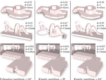
Exhautive partition + GC Kinetic partition + IP Kinetic partition + GC e=0.33 s=0.44 t=56sec e=0.42 s=1.04 t=42sec e=0.38 s=1 t=43sec e=0.41 s=0.12 t=12min e=0.67 s=0.98 t=3.5min e=0.29 s=0.94 t=1.8min e=0.052 s=0.24 t=4.6hrs e=0.062 s=1.49 t=16min e=0.057 s=1.63 t=15min

Fig. 15. Ablation study. Combining exhaustive partitions with our graph-cut (GC) solver produces accurate models resulting from the exploration of a large solution space. However, this combination is not time-efficient and returns models with a low simplicity score illustrated by numerous visual artifacts (left). Plugging the integer programming (IP) solver of Polyfit on kinetic partitions is a more efficient -yet less accurate- option (middle). Our framework offers the best performances and also the best compromise between accuracy and output simplicity (right). Models from Figure 14.

Comparisons with surface reconstruction methods. We compared our algorithm with Polyfit [Nan and Wonka 2017] and Chauve’s method [Chauve et al. 2010], which are arguably the two most robust existing methods in the field. To fairly compare the reconstruction

e= 0.49 s_{= 0.4} t= 115 m= 1.4 Chauve e= 0.54 s_{= 0.76} t= 296 m= 1.6 Polyfit e= 0.48 s_{= 0.82} t= 31 m= 0.08 Ours

Fig. 16. Comparisons with reconstruction methods. Starting from the same 75 planar shapes, Chauve’s method [Chauve et al. 2010] and Polyfit [Nan and Wonka 2017] are both more time- and memory-consuming than our algorithm while delivering less concise polygonal meshes, both less accurate and less compact. e, s, t and m correspond to the symmetric mean Hausdorff error (in % of the bounding box diagonal), simplicity, running time (in sec) and memory peak (in GB) respectively. The colored point clouds show the error distribution (yellow=0, black≥ 1% of the bounding box diagonal).

mechanisms, we used the same configuration of planar shapes for all methods. In particular, we deactivated the shape completion module in Chauve’s method. Figure 16 shows the results obtained on Hand from 75 planar shapes. Because Polyfit and Chauve’s method naively slice the object bounding box by the planar shapes, they produce overly-dense partitions. For example, their exhaustive partition for Hand is composed of 30K cells and 91K facets, whereas our partition contains 0.7K cells and 3.5K facets only. Extracting output surface from a much lighter partition thus becomes faster and less memory-consuming. Our algorithm also outperforms Polyfit and Chauve’s method in terms of fidelity and simplicity. Our surface extraction is more efficient in balancing between fidelity and simplicity. The main reason relies on the use of a simpler data term where only inlier points are taken into account to measure the faithfulness. This technical choice offers more robustness to imperfect data than the visibility criterion of Chauve’s method and more stability than the three-term energy of Polyfit.

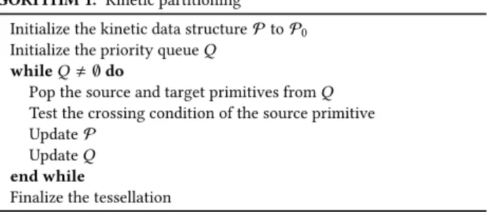
Graphs presented in Figure 17 compared the scalability of the methods. Polyfit in its Gurobi solver version may require days of computing when more than one hundred planar shapes are handled whereas Chauve’s method exceeds 32GB memory for processing slightly more than two hundred shapes. In particular, the former ex-ploits a time-consuming integer programming solver while the latter suffers from a memory-consuming visibility estimation. Conversely, our algorithm with no subdivision scheme can process one thousand planar shapes under more reasonable processing times and without exceeding 32GB memory. More qualitative and quantitative results are provided in supplementary material and in [Bauchet 2019].

Comparisons with surface approximation pipelines. We also com-pared our algorithm with the surface approximation methods QEM [Garland and Heckbert 1997], SAMD [Salinas et al. 2015] and VSA [Cohen-Steiner et al. 2004]. Because these methods operate from

10 102 103 104 105 Ours Chauve Polyfit Running time ( s.)

Number of planar shapes

0 200 400 600 800 1000 10 102 103 104 Memor y p eak (MB.)

Number of planar shapes

0 200 400 600 800 1000

Fig. 17. Performances of surface reconstruction methods. Polyfit [Nan and Wonka 2017] requires days of computing for assembling one hundred shapes, whereas Chauve’s method [Chauve et al. 2010] exceeds 32GB memory for slightly more than two hundred shapes. Our algorithm is one order magni-tude more scalable than these two methods. Tests have been performed on the Hand model (Fig.16) without using subdivision schemes.

meshes, we first reconstructed a dense triangle mesh from input points using the screened Poisson algorithm [Kazhdan and Hoppe 2013]. Both a freeform object (Fertility) and a nearly piecewise-planar structure (Lans) were used for this comparison. As shown in Figure 18, polyhedral meshes produced by our algorithm are geometrically more accurate than those returned by these three methods at a similar mesh complexity, i.e. with the same number of output facets. The accuracy gain is particularly high at low mesh complexity where approximation methods cannot capture correctly the structure of the object and tend to shrink the output surface. By operating directly from input points, our algorithm does not de-pend on an intermediate dense mesh reconstruction step in which geometric and topological errors are likely to occur. Moreover, the large polygonal facets returned by our algorithm approximate the object more effectively than the triangle facets returned by edge contraction (QEM and SAMD) or constrained Delaunay triangula-tion built from a primitive connectivity graph (VSA). In terms of performance, the approximation pipelines have similar processing times and memory consumption than our algorithm when produc-ing low complexity meshes. For instance, the four methods process the Lans model with 25 output facets (see bottom row in Figure 18) in approximately half a minute. High complexity meshes, i.e. with more than 200 facets, are produced more quickly by the ap-proximation pipelines than by our algorithm. More qualitative and quantitative results can be found in supplementary material.

Limitations. Our work focuses on assembling planar shapes, not on detecting them. We assume planar shapes can be accurately detected from input points by standard algorithms. However, this

assumption might be wrong in presence of data highly corrupted by noise and severe occlusions. For such cases, configurations of planar shapes returned by existing algorithms are typically inaccu-rate and incomplete. Our kinetic algorithm can only correct con-figurations where missing planar shapes are parts of a repetitive structure as illustrated in Figure 5. Our surface extraction solver is also not designed to reconstruct non-manifold geometry where some object parts have no thickness. By using an inside-outside labeling, our solver forces each object part to have a non-zero thick-ness. Consequently, a non-manifold object will be either shrunk or overly-simplified around its zero thickness components. For such objects, the flexibility of an integer programming solver is probably a better choice here. Finally, the initialization of non-convex shapes by their convex hulls can create extra cuttings. One solution to build even lighter partitions could be to decompose their alpha-shapes into convex polygons. Increasing the number of polygons would however decrease performances.

7 APPLICATION TO CITY MODELING

We now show how our algorithm can be used in a concrete applica-tion such as city modeling from airborne Lidar data. City modeling mainly consists in reconstructing buildings with a piecewise-planar geometry [Musialski et al. 2013]. Before applying our algorithm, we first need to distinguish buildings from other urban objects con-tained in Lidar scans. We relied on the classification package of the CGAL Library [Giraudot and Lafarge 2019] for this task. We considered three classes of interest:building, ground and other. We ran the Random Forest classifier with the default geometric features. As second step, we then detected planar shapes from points labeled asbuilding. Because Lidar scans are typically acquired at nadir, fa-cades are mostly occluded and not captured by planar shapes. We thus consolidated the set of detected shapes by adding artificial vertical planar shapes at the building contours. We computed an elevation map (or Digital Surface Model) from the raw Lidar scan by planimetric projection and detect line-segments located along high gradients by the LSD algorithm [Von Gioi et al. 2010]. The 2D line-segments were finally lifted into vertical rectangles to form the set of extra planar shapes. The last step consisted in applying our kinetic partitioning and surface extraction from the consolidated set of planar shapes. Figure 19 illustrates these steps on the city of Den-vers, US. The output mesh is both compact with only 12.9K facets for describing 703 buildings, and accurate with a mean Hausdorff distance to the input points labeled asbuilding of 0.52 meter.

8 CONCLUSION

We proposed an algorithm for converting point clouds into concise polygonal meshes. The key technical ingredient of the algorithm is a kinetic data structure where planar shapes grow at constant speed until colliding and partitioning the space into a low number of polyhedra. This idea does not only bring efficiency and scala-bility with respect to existing methods, it also allows us to deliver more concise polygonal meshes extracted from lighter yet more meaningful partition of polyhedra. We demonstrated the robust-ness and efficiency of our algorithm on a variety of objects and scenes in terms of complexity, size and acquisition characteristics.

QEM SAMD VSA Ours 0 200 400 600 800 1000 0 0.5 1.0 1.5 Ge ometric err or Number of facets 0 200 400 600 800 1000 0 0.5 1.0 1.5 Ge ometric err or Number of facets Ours QEM SAMD VSA # f =25 # f =175 # f =100 # f =1,000

Fig. 18. Comparisons with surface approximation methods. The left curves, that measure the geometric error in function of the number of facets of the output mesh, show that our algorithm outclasses simplification methods for both a freeform object (Fertility, top) and a nearly piecewise planar structure (Lans, bottom). QEM [Garland and Heckbert 1997] cannot output large meaningful facets whereas SAMD [Salinas et al. 2015] and VSA [Cohen-Steiner et al. 2004] fail to correct the geometric inaccuracies contained in the dense triangle mesh. For each row, the four meshes contain the same number of facets #f. The geometric error is measured as the symmetric mean Hausdorff distance between input points and output mesh.

We also showed the applicability of our algorithm in city modeling for reconstructing large-scale airborne Lidar scans.

In future work, we will generalize the kinetic partitioning algo-rithm to non-planar shapes using NURBS and other parametric functions. Although the collision detection for such shapes is even more challenging to compute efficiently, this perspective would allow us to reconstruct freeform objects with a better complexity-distortion tradeoff. We also plan to investigate the potential of our kinetic data structure for repairing CAD models.

ACKNOWLEDGMENTS

This project was partially funded by Luxcarta Technology. We thank our anonymous reviewers for their input, Qian-Yi Zhou and Arno Knapitsch for providing us datasets from the Tanks and Temples benchmark (Meeting Room, Horse, M60, Barn, Ignatius, Court-house and Church), and Pierre Alliez, Mathieu Desbrun and George Drettakis for their help and advice. We are also grateful to Lian-gliang Nan and Hao Fang for sharing comparison materials. Datasets Full thing, Castle, Tower of Pi and Hilbert cube originate from Thingi10K, Hand, Rocker Arm, Fertility and Lans from Aim@Shape, and Stanford Bunny and Asian Dragon from the Stanford 3D Scanning Repository.

REFERENCES

Pankaj K. Agarwal, Jie Gao, Leonidas J. Guibas, Haim Kaplan, Vladlen Koltun, Natan Rubin, and Micha Sharir. 2010. Kinetic stable Delaunay graphs. InProc. of Symposium on Computational Geometry (SoCG).

Murat Arikan, Michael Schwarzler, Simon Flory, Michael Wimmer, and Stefan Maier-hofer. 2013. O-Snap: Optimization-Based Snapping for Modeling Architecture._Trans. on Graphics 32, 1 (2013).

Julien Basch, Jeff Erickson, Leonidas J. Guibas, John Hershberger, and Li Zhang. 2004. Kinetic collision detection between two simple polygons.Computational Geometry 27, 3 (2004).

Jean-Philippe Bauchet. 2019.Kinetic data structures for the geometric modeling of urban environments. PhD thesis. Université Côte d’Azur, France.

Jean-Philippe Bauchet and Florent Lafarge. 2018. KIPPI: KInetic Polygonal Partitioning of Images. InProc. of Computer Vision and Pattern Recognition (CVPR).

Matthew Berger, Andrea Tagliasacchi, Lee M. Seversky, Pierre Alliez, Gael Guennebaud, Joshua A. Levine, Andrei Sharf, and Claudio T. Silva. 2017.A Survey of Surface Reconstruction from Point Clouds._{Computer Graphics Forum 36, 1 (2017).} Andras Bodis-Szomoru, Hayko Riemenschneider, and Luc Van Gool. 2015. Superpixel

meshes for fast edge-preserving surface reconstruction. In_{Proc. of Computer Vision} and Pattern Recognition (CVPR).

Mario Botsch, Leif Kobbelt, Mark Pauly, Pierre Alliez, and Bruno Lévy. 2010._Polygon Mesh Processing.

Alexandre Boulch, Martin De La Gorce, and Renaud Marlet. 2014. Piecewise-Planar 3D Reconstruction with Edge and Corner Regularization._{Computer Graphics Forum 33,} 5 (2014).

Yuri Boykov and Vladimir Kolmogorov. 2004. An Experimental Comparison of Min-Cut/Max-Flow Algorithms for Energy Minimization in Vision._{Trans. on Pattern} Analysis and Machine Intelligence (PAMI) 26, 9 (2004).

Anne-Laure Chauve, Patrick Labatut, and Jean-Philippe Pons. 2010. Robust Piecewise-Planar 3D Reconstruction and Completion from Large-Scale Unstructured Point Data. InProc. of Computer Vision and Pattern Recognition (CVPR).

Desai Chen, Pitchaya Sitthi-Amorn, Justin T. Lan, and Wojciech Matusik. 2013. Com-puting and fabricating multiplanar models. InComputer Graphics Forum, Vol. 32. Jie Chen and Baoquan Chen. 2008.Architectural Modeling from Sparsely Scanned

Range Data.International Journal of Computer Vision (IJCV) 78, 2-3 (2008). David Cohen-Steiner, Pierre Alliez, and Mathieu Desbrun. 2004. Variational Shape

Approximation. InProc. of SIGGRAPH.

James M. Coughlan and Alan L. Yuille. 2000. The Manhattan world assumption: Reg-ularities in scene statistics which enable Bayesian inference. InProc. of Neural Information Processing Systems.

Guillaume Damiand. 2018. Combinatorial Maps. In_{CGAL User and Reference Manual} (4.14 ed.). CGAL Editorial Board.

Hao Fang, Florent Lafarge, and Mathieu Desbrun. 2018. Planar Shape Detection at Structural Scales. In_{Proc. of Computer Vision and Pattern Recognition (CVPR).}

Fig. 19. Application to city modeling. We use our algorithm to reconstruct the downtown of Denvers, US from a Airbone Lidar scan of 15.1M points. After classifying input points into ground in grey, building in red and other in green (top left point cloud) and after detecting 13K planar shapes from building and

groundpoints (bottom left set of polygons), our algorithm reconstructs the 703 buildings of the scene with a CityGML-LOD2 representation (right). The

output mesh is composed of 12.9K facets only.

Michael Garland and Paul S. Heckbert. 1997. Surface simplification using quadric error metrics. InProc. of SIGGRAPH.

Simon Giraudot and Florent Lafarge. 2019. Classification. InCGAL User and Reference Manual (4.14 ed.). CGAL Editorial Board.

Leonidas J. Guibas. 2004. Kinetic data structures. InHandbook of Data Structures and Applications.

Leonidas J. Guibas, Lyle Ramshaw, and Jorge Stolfi. 1983.A kinetic framework for computational geometry. In_{Symposium on Foundations of Computer Science.} LLC Gurobi Optimization. 2019. Gurobi Optimizer Reference Manual.

Thomas Holzmann, Michael Maurer, Friedrich Fraundorfer, and Horst Bischof. 2018. Semantically Aware Urban 3D Reconstructionwith Plane-Based Regularization. In Proc. of European Conference on Computer Vision (ECCV).

Jin Huang, Tengfei Jiang, Zeyun Shi, Yiying Tong, Hujun Bao, and Mathieu Desbrun. 2014.L1-Based Construction of Polycube Maps from Complex Shapes.Trans. on

Graphics 33, 3 (2014).

Satoshi Ikehata, Hang Yan, and Yasutaka Furukawa. 2015. Structured Indoor Modeling. InInternational Conference on Computer Vision (ICCV).

Caigui Jiang, Chengcheng Tang, Amir Vaxman, Peter Wonka, and Helmut Pottmann. 2015. Polyhedral Patterns.Trans. on Graphics 34, 6 (2015).

Caigui Jiang, Jun Wang, Johannes Wallner, and Helmut Pottmann. 2014.Freeform Honeycomb Structures.Computer Graphics Forum 33 (2014).

Adrien Kaiser, Jose Alonso Ybanez Zepeda, and Tamy Boubekeur. 2018. A Survey of Simple Geometric Primitives Detection Methods for Captured 3D Data.Computer Graphics Forum 37 (2018).

Michael Kazhdan, Matthew Bolitho, and Hughes Hoppe. 2006. Poisson surface recon-struction. InSymposium on Geometry Processing.

Michael Kazhdan and Hugues Hoppe. 2013. Screened poisson surface reconstruction. Trans. on Graphics 32, 3 (2013).

Arno Knapitsch, Jaesik Park, Qian-Yi Zhou, and Vladlen Koltun. 2017. Tanks and Temples: Benchmarking Large-Scale Scene Reconstruction._{Trans. on Graphics 36, 4} (2017).

Patrick Labatut, Jean-Philippe Pons, and Renaud Keriven. 2009. Robust and Efficient Surface Reconstruction From Range Data._{Computer Graphics Forum 28, 8 (2009).} Florent Lafarge and Pierre Alliez. 2013. Surface reconstruction through point set

structuring. In_{Computer Graphics Forum, Vol. 32.}

Lingxiao Li, Minhyuk Sung, Anastasia Dubrovina, Li Yi, and Leonidas Guibas. 2019. Supervised Fitting of Geometric Primitives to 3D Point Clouds . In_{Proc. of Computer} Vision and Pattern Recognition (CVPR).

Yangyan Li, Xiaokun Wu, Yiorgos Chrysathou, Andrei Sharf, Daniel Cohen-Or, and Niloy J. Mitra. 2011. GlobFit: consistently fitting primitives by discovering global relations. InTrans. on Graphics, Vol. 30.

Peter Lindstrom. 2000. Out-of-core Simplification of Large Polygonal Models. InProc. of SIGGRAPH.

David Marshall, Gabor Lukacs, and Ralph Martin. 2001. Robust Segmentation of Primitives from Range Data in the Presence of Geometric Degeneracy.Trans. on

Pattern Analysis and Machine Intelligence (PAMI) 23, 3 (2001).

Aron Monszpart, Nicolas Mellado, Gabriel J. Brostow, and Niloy J. Mitra. 2015. Rapter: Rebuilding man-made scenes with regular arrangements of planes.Trans. on Graph-ics 34, 4 (2015).

Claudio Mura, Oliver Mattausch, and Renato Pajarola. 2016. Piecewise-planar Recon-struction of Multi-room Interiors with Arbitrary Wall Arrangements._Computer Graphics Forum 35, 7 (2016).

T. Murali and Thomas Funkhouser. 1997. Consistent Solid and Boundary Representa-tions from Arbitrary Polygonal Data. In_{Symposium on Interactive 3D Graphics.} Przemyslaw Musialski, Peter Wonka, Daniel G. Aliaga, Manuel Wimmer, Luc Van Gool,

and Werner Purgathofer. 2013. A Survey of Urban Reconstruction. _Computer Graphics Forum 32, 6 (2013).

Liangliang Nan and Peter Wonka. 2017. PolyFit: Polygonal surface reconstruction from point clouds. In_{Proc. of International Conference on Computer Vision (ICCV).} Sven Oesau, Florent Lafarge, and Pierre Alliez. 2016. Planar shape detection and

regularization in tandem. InComputer Graphics Forum, Vol. 35.

Sven Oesau, Yannick Verdie, Clément Jamin, Pierre Alliez, Florent Lafarge, and Simon Giraudot. 2018.Point Set Shape Detection.InCGAL User and Reference Manual (4.14 ed.). CGAL Editorial Board.

Tahir Rabbani, Frank Van Den Heuvel, and George Vosselman. 2006. Segmentation of point clouds using smoothness constraint.ISPRS 36, 5 (2006).

David Salinas, Florent Lafarge, and Pierre Alliez. 2015. Structure-Aware Mesh Decima-tion.Computer Graphics Forum 34, 6 (2015).

Falko Schindler, Wolfgang Worstner, and Jan-Michael Frahm. 2011. Classification and Reconstruction of Surfaces from Point Clouds of Man-made Objects. InProc. of International Conference on Computer Vision (ICCV) Workshops.

Ruwen Schnabel, Patrick Degener, and Reinhard Klein. 2009. Completion and recon-struction with primitive shapes. In_{Computer Graphics Forum, Vol. 28.}

Ruwen Schnabel, Roland Wahl, and Reinhard Klein. 2007. Efficient RANSAC for point-cloud shape detection. In_{Computer Graphics Forum, Vol. 26.}

Johannes Lutz Schönberger and Jan-Michael Frahm. 2016. Structure-from-Motion Revisited. In_{Proc. of Computer Vision and Pattern Recognition (CVPR).}

Marco Tarini, Kai Hormann, Paolo Cignoni, and Claudio Montani. 2004. PolyCube-Maps. Trans. on Graphics 23, 3 (2004).

Marc Van Kreveld, Thijs Van Lankveld, and Remco C. Veltkamp. 2011. On the shape of a set of points and lines in the plane._{Computer Graphics Forum 30 (2011).} Yannick Verdie, Florent Lafarge, and Pierre Alliez. 2015. LOD Generation for Urban

Scenes._{Trans. on Graphics 34, 3 (2015).}

Rafael Von Gioi, Jeremie Jakubowicz, Jean-Michel Morel, and Gregory Randall. 2010. LSD: A fast line segment detector with a false detection control.Trans. on Pattern Analysis and Machine Intelligence (PAMI) 32, 4 (2010).

Qingnan Zhou and Alec Jacobson. 2016. Thingi10K: A Dataset of 10, 000 3D-Printing Models.arXiv:1605.04797 (2016).