HAL Id: hal-00682695
https://hal.archives-ouvertes.fr/hal-00682695
Submitted on 29 Mar 2012HAL is a multi-disciplinary open access archive for the deposit and dissemination of sci-entific research documents, whether they are pub-lished or not. The documents may come from teaching and research institutions in France or abroad, or from public or private research centers.
L’archive ouverte pluridisciplinaire HAL, est destinée au dépôt et à la diffusion de documents scientifiques de niveau recherche, publiés ou non, émanant des établissements d’enseignement et de recherche français ou étrangers, des laboratoires publics ou privés.
LINEAR APPROXIMATION OF OPEN-CHANNEL
FLOW ROUTING WITH BACKWATER EFFECT
Simon Munier, Xavier Litrico, Gilles Belaud
To cite this version:
Simon Munier, Xavier Litrico, Gilles Belaud. LINEAR APPROXIMATION OF OPEN-CHANNEL FLOW ROUTING WITH BACKWATER EFFECT. 32nd Congress of the International Association of Hydraulic Engineering and Research, 2007, Venice, Italy. 10p. �hal-00682695�
LINEAR APPROXIMATION OF OPEN-CHANNEL
FLOW ROUTING WITH BACKWATER EFFECT
Simon Munier(1), Xavier Litrico(1), Gilles Belaud(2)
(1) Cemagref, UMR G-EAU, B.P. 5095, 34196 Montpellier Cedex 5, France,
phone: +33 467 04 63 47, fax: +33 467 16 64 40, e-mail: [email protected], [email protected]
(2) Sup’Agro, UMR G-EAU, 2 place Viala, 34060 Montpellier, France,
phone: +33 499 61 24 23, fax: , e-mail: [email protected]
ABSTRACT
This paper proposes a new model for linear flow routing in open-channels. The proposed model, called LBLR for Linear Backwater Lag and Route, is a first order with delay model that explicitly takes into account two parameters which are usually neglected: 1) the downstream boundary condition and 2) the nonuniform flow conditions, both of which are shown to have a strong influence on the flow dynamics. The model parameters are obtained analytically from the pool characteristics (geometry, friction, discharge and downstream boundary condition). A frequency domain approach is used to compute the frequency response of the linearized Saint-Venant equations. This model is then approximated by a first order plus delay model using the moment matching method. The proposed model is shown to perform better than existing models when the flow is affected by backwater and/or by different downstream boundary conditions from the one corresponding to uniform flow.
Keywords: Open-channel flow, Laplace transform, frequency response, Saint-Venant
equations, time-delay, flow routing.
1 INTRODUCTION
Modelling of the flow routing in a river stretch has been the subject of numerous publications since the 1950’s. Weinmann and Laurenson (1979) presented a comprehen-sive review of approximate flow routing methods and showed that all available methods are derived from either kinematic wave or diffusion analogy models. Different linear models have been developed for flow routing simulation purposes (see e.g. Dooge et al. (1987a); Moussa (1996); Tsai (2003)). Most of them are based on an analysis of linearized Saint-Venant equations around uniform flow conditions, and also neglect the effect of the downstream boundary condition by considering a semi-infinite channel. Such a limitation may lead to bad results in flow forecasting, even for small discharge variations (i.e. even in a linear framework). For instance, mild slope channels or low flows in channels including hydraulic structures may cause non-negligible backwater effects.
In this paper, we propose to consider separately the effects of open-channel dynamics and of the downstream boundary condition. We show that the same channel will not react identically when one changes its downstream boundary condition, which is imposed by a hydraulic structure (e.g. by a weir).
To this purpose, we consider the linearized complete Saint-Venant equations, then we use a frequency domain approach to represent those equations by transfer functions in the Laplace domain. In this framework, the introduction of a downstream boundary condition is equivalent to a local feedback between the discharge and the water level deviations. A moment matching method is then used to compute the parameters of a first order plus delay model that approximates the system in low frequencies. The obtained model, called LBLR for Linear Backwater Lag and Route, is first computed in the uniform case, then extended to the nonuniform one. In the last section, the model is validated on an example canal with different dynamic behavior.
2 PROBLEM STATEMENT
For flow routing models applied on rivers stretches or on channels, a non-realistic as-sumption is usually made, which is to neglect the downstream boundary condition. This is achieved by considering two other assumptions: uniform flow and semi-infinite channel. Yet, there are always singularities in the channel, such as weirs for instance, which modify its dynamic behavior. In that sense these two generally admitted assumptions can some-times lead to important errors in the model’s results. In particular, the delay time, one of the most important values to be estimated in a context of water resources management, can be shown to depend on the downstream boundary condition.
In this paper, we first consider the complete Saint-Venant equations for a prismatic channel, then we linearize them around a nonuniform stationary flow. Independently, we explicitly take the downstream local feedback into account which links the discharge to the water depth at the downstream end of the channel. Coupling the effects of open-channel dynamics and of the downstream local feedback enables us to consider the influence of hydraulic structures on a nonuniform flow.
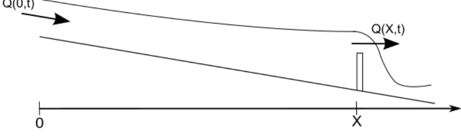
Figure 1: General scheme of the considered channel
3 LINEARIZED MODEL OF AN OPEN-CHANNEL
We consider a canal pool of length X meters with prismatic geometry, with the input and output discharges as boundary conditions (see fig. 1). The Saint-Venant equations are stated for such a canal pool, we then linearize these equations, and give the solution in the frequency domain, leading to the Saint-Venant transfer matrix.
We use the following notations to describe the flow: A(x, t) is the wetted area (m2),
P (x, t) the wetted perimeter (m), Q(x, t) the discharge (m3/s) across section A (m2),
Y (x, t) the water depth (m), Sb the bed slope, Sf the friction slope, F = V /C the Froude
number with C = √gA/T the wave celerity (ms−1), V = Q/A the flow velocity (ms−1),
the flow is assumed to be subcritical (i.e. F < 1). Equilibrium variables are denoted with a subscript zero (Q0(x), Y0(x), F0, Sf 0, etc.).
3.1 LINEARIZED SAINT-VENANT EQUATIONS
The Saint-Venant equations are first order hyperbolic nonlinear partial differential equations (Chow (1988)). We consider small variations of discharge q(x, t) and water depth y(x, t) around a nonuniform stationary regime, defined by Q0(x) = Q0 and Y0(x), solution of the following ordinary differential equation for a boundary condition defined by downstream elevation Y0(X): dY0(x) dx = Sb − Sf 0(x) 1− F0(x)2 (1) The linearized Saint-Venant equations are given by (see Litrico and Fromion (2004a) for details): T0(x) ∂y ∂t + ∂q ∂x = 0 (2) ∂q ∂t + 2V0(x) ∂q ∂x − β0(x)q + (C 2 0(x)− V 2 0(x))T0(x) ∂y ∂x − γ0(x)y = 0 (3)
Parameters γ0 and β0 are defined by (dependance on x is omitted for readability):
γ0 = V02 dT0 dx + gT0 [ (1 + κ0)Sb− (1 + κ0− (κ0− 2)F02) dY0 dx ] (4) β0 = − 2g V0 ( Sb− dY0 dx ) (5) with κ0 = 7/3− 4A0/(3T0P0)(∂P/∂Y )0.
The boundary conditions are the upstream and downstream discharges q(0, t) and
q(X, t).
3.2 SAINT-VENANT TRANSFER MATRIX
3.2.1 Uniform flow
Applying Laplace transform to the linear partial differential equations (2–3) results in a system of Ordinary Differential Equations in the variable x, parameterized by the Laplace variable s, which leads, in the uniform case, to the open-loop Saint-Venant dis-tributed transfer matrix G(x, X, s) relating the water depth y(x, s) and the discharge
q(x, s) at any point x in the canal pool to the upstream and downstream discharges (see
Litrico and Fromion (2006) for details): ( y(x, s) q(x, s) ) = ( λ2eλ2x+λ1X−λ1eλ1x+λ2X T0s(eλ2X−eλ1X) λ1eλ1x−λ2eλ2x T0s(eλ2X−eλ1X) eλ1x+λ2X−eλ2x+λ1X eλ2X−eλ1X eλ2x−eλ1x eλ2X−eλ1X ) | {z } gij(x,X,s) ( q(0, s) q(X, s) ) (6)
where λ1 and λ2 are given by:
λi(s) = 2T0V0s + γ0+ (−1)i √ 4C2 0T02s2 + 4T0(V0γ0− (C02− V02)T0β0)s + γ02 2T0(C02− V02) (7)
Let us note that usually, when considering a semi-infinite channel, one tries to eval-uate the discharge at the downstream end, knowing the discharge at the upstream end. Making the assumption of a semi-infinite channel is equivalent to taking X → ∞. Hence, as far as x represents the length of the channel, equation (6) leads to the transfer func-tion given by Dooge et al. (1987a): q(x, jω) = eλ1xq(0, jω), since Re[λ
1(jω)] < 0 and
Re[λ2(jω)] > 0.
On the other hand, considering a downstream boundary condition adds a relation between the discharge and the water depth at the downstream end of the channel. Only the boundary variables are then considered (x = 0 or x = X), and equation (6) leads to the input-output Saint-Venant transfer matrix denoted P (X, s) = (pij(X, s)), with:
( y(0, s) y(X, s) ) = ( g11(0, X, s) g12(0, X, s) g11(X, X, s) g12(X, X, s) ) | {z } pij(X,s) ( q(0, s) q(X, s) ) (8) 3.2.2 Nonuniform flow
Based on an idea initially proposed by Schuurmans et al. (1999), and modified by Litrico and Fromion (2004b), we approximate a channel with backwater by the interaction of two pools. This is based on the approximation of the backwater curve by a stepwise linear function: a line parallel to the bed in the upstream part (corresponding to the uni-form part) and a line tangent to the real curve at the downstream end in the downstream part. Let x1 denote the abscissa of the intersection of the two lines. The corresponding approximation of the backwater profile is schematized in figure 2.
Figure 2: Backwater curve approximation scheme
After having divided the pool into two parts, a transfer matrix can be established for each sub-pool. The transfer matrix of the whole pool is then given by (see Litrico and Fromion (2004b)): ˆ P = ( ˆ p11 pˆ12 ˆ p21 pˆ22 ) = ( p11+p¯p1112−pp2122 −p¯p1112−pp¯1222 p21p¯21 ¯ p11−p22 p¯22− ¯ p12p¯21 ¯ p11−p22 ) (9) where pij denote the terms of the matrix corresponding to the upstream part and ¯pij
those corresponding to the downstream part, and ˆP the transfer matrix corresponding to
3.3 COUPLING WITH A DOWNSTREAM BOUNDARY CONDITION We now consider an open-channel with a given downstream boundary condition ex-pressed as a local coupling between the discharge and the water elevation. This condition can either be due to a hydraulic structure, or to the effect of a semi-infinite channel.
In any case, linearizing the relation between the discharge and the water depth leads to the following equation, expressed in the Laplace domain:
q(X, s) = ky(X, s) (10)
where k represents the local feedback (k = (dQ/dY )0).
For example, a weir is usually described by the following free flow equation:
Q(X, t) = Cd
√
2gLw(Y (X, t)− Zs)3/2 (11)
where Cd is the discharge coefficient, Lw the weir length, Zs the sill elevation and g the
gravitational acceleration. If Cdremains constant, the feedback parameter k is given here
by: k = 32 Q0
Y0(X)−Zs.
One may note that a semi-infinite channel can also be simulated by choosing a coeffi-cient k that approximates the non-reflective boundary condition (see Litrico and Fromion (2006) for details).
3.4 COMPLETE LINEAR MODEL FOR FLOW ROUTING
In section 3.2, we established the linearized Saint-Venant transfer matrix for a nonuni-form flow. Independently we presented a linearized expression of the downstream bound-ary condition in section 3.3. It is now possible to combine the flow routing effects (transfer matrix given by eq. (9)) with the feedback effects (eq. (10)), which leads to:
q(X, s) = k ˆp21(X, s)
1− kˆp22(X, s)
q(0, s) (12)
This equation provides an accurate linear model for flow transfer in an open-channel with a given downstream boundary condition.
4 APPROXIMATE LINEAR MODEL FOR FLOW ROUTING
4.1 MOMENT MATCHING METHOD
4.1.1 Uniform flow
The transfer function of the complete linear model given by equation (12) can be transposed to the uniform case by replacing the transfer matrix ˆP by P . Then the transfer function for uniform flow and downstream local feedback is given by:
q(X, s) = kp21(s)
1− kp22(s)
q(0, s) (13)
Following the classical moment matching method (see e.g. Dooge et al. (1987b); Rey (1990)) the transfer function (13) can be approximated by a first order with delay transfer function given by:
q(X, s) = e
−τs
We use the following definition of the R-th logarithmic moments of the transfer function h expressed in the Laplace domain:
MR[h] = (−1)R
dR
dsR{log[h(s)]}s=0 (15)
Equating the two first moments of transfer functions (13) and (14) leads to:
τ + K = M1 (16)
K2 = M2 (17)
where M1 and M2 are the first and second order logarithmic moments of the transfer function (13).
Finally, we obtain an analytical expression of K and τ for the case of uniform flow:
K = √1 2b [( c +T k ( a + T 2k ) ( 1− e−2bX ) + ( ad 2b + T d 2kb ) ( 1 + e−2bX )) + a 2 2 (1 + e −4bX) + d 2X 2b (1 + 2e −2bX) + d2 8b2(−5 + 4e−2bX + e−4bX)− 2bcX − 2dX ( a + T k ) e−2bX ] (18) τ = 1 2b [( a− d 2b + T k ) (1− e−2bX) + dX − 2abX ] (19) where: a = V0 C2 0−V02, b = γ0 2T0(C02−V02), c = C2 0 (C2 0−V02)2, d = V0γ0−(C02−V02)T0β0 T0(C02−V02)2 .
Equations (18-19) provide the best low frequency approximation of the flow transfer by a first order with delay. Parameters are obtained analytically as functions of the downstream boundary condition k and the physical parameters of the pool. In the next section we show that the extension of this method to the nonuniform case provides similar results.
4.1.2 Nonuniform flow
The moment matching method can be applied between the transfer function given by (12) and a first order with delay. Equation (9), giving expressions of ˆpij, allows us to
rewrite the complete transfer function ˆh(k, X, s) (given by (12)) as follows (dependance
on (k, X, s) is omitted for more readability): ˆ
h = k ˆp21
1− kˆp22
= kp21p¯21
ZP ¯P (20)
where p21, ¯p21 and ZP ¯P = (¯p11− p22)(1− k¯p22) + k ¯p12p¯21 respectively represent the con-tribution of the uniform part, of the backwater part and of the interaction between the two parts of the pool.
Considering the low frequencies approximation (s→ 0), one can write: log ˆh = ˆM0− ˆM1s + ˆM2
s2
2 + O(s
3) (21)
Applying this approximation to the three contributions p21, ¯p21 and ZP ¯P leads to the
following expression of the transfer function logarithmic moments: ˆ
Mi = M21,i+ ¯M21,i− MZP ¯P,i , i = 0, 1, 2 (22)
where M21,i, ¯M21,i and MZP ¯P,i are the i-th logarithmic moments of p21, ¯p21 and ZP ¯P
respectively. These moments can be computed by Taylor series expansion around s = 0. Solving (22) leads to closed-form expressions of ˆK and ˆτ , explicitly depending on the
pool characteristics (geometry, friction, discharge, downstream water depth and feedback parameter).
Finally, as for the uniform case, we established an approximated model (a first order plus delay) for a nonuniform flow including backwater effects. The two parameters ˆK
and ˆτ are obtained as closed-form analytical expressions of the pool characteristics, easily
computable.
4.2 ILLUSTRATION ON AN EXAMPLE CHANNEL
We simulate a propagation of a step discharge change at x = 0, with a trapezoidal prismatic channel, with characteristics detailed in table 1, where X is the channel length (m), m the bank slope, B the bed width (m), Sb the bed slope, n the Manning roughness
coefficient (m−1/3s), Yn the uniform depth (m) corresponding to the reference discharge
Qr (m3s−1).
Table 1: Parameters for the example canal
X m B Sb n Yn Qr
6000 1.5 8 0.0008 0.02 2.92 80
In order to validate our model and analyze the feedback effects, different situations have been simulated on this example canal with three different models. The first one is the linearized Saint-Venant model which is used as a reference for linear flow transfer. It is simulated with an accurate rational model obtained from frequency response of Saint-Venant linearized equations (see Litrico and Fromion (2004a)). The second one is a linear lag and route model (called LLR), a first order with delay established with the uniform flow assumption and the semi-infinite channel approximation, and which consequently does not take the downstream boundary condition into account. The third one is our model, the LBLR.
4.2.1 Simulation in uniform flow
The first situation represents a uniform canal, which is achieved by choosing for the feedback parameter k a suitable value that allows the simulation of a semi-infinite canal. The Bode diagram and the step response for this case are represented on fig. 3. These graphs show that the three curves are very similar in the time domain, and in the low frequencies in the frequency domain. The small difference between the LLR model and the LBLR one comes from the choice of k which is an approximation of the exact value corresponding to the semi-infinite canal assumption.
10−5 10−4 10−3 10−2 −40 −30 −20 −10 0 frequency (rad/s) magnitude (dB) 10−5 10−4 10−3 10−2 −500 −400 −300 −200 −100 0 frequency (rad/s) phase (deg) 0 50 100 150 0 0.5 1 time (min) downstream discharge (m 3 /s) Saint−Venant LLR LBLR
Figure 3: Bode diagram and step response for the example canal in the uniform case
10−5 10−4 10−3 10−2 −40 −30 −20 −10 0 frequency (rad/s) magnitude (dB) 10−5 10−4 10−3 10−2 −500 −400 −300 −200 −100 0 frequency (rad/s) phase (deg) 0 50 100 150 0 0.5 1 time (min) downstream discharge (m 3 /s) Saint−Venant LLR LBLR increasing k
Figure 4: Bode diagram for the example canal with a local feedback and step response for different values of k
4.2.2 Effects of the downstream boundary condition
In the second situation, we consider the effect of the downstream local feedback by fixing a value for the parameter k, which can represent any structure with any character-istics at the downstream end of the pool. Fig. 4 shows the Bode diagram for which the value k = 18 has been chosen, and the step response for three different values of k (10, 25 and 250). These values may correspond to different structures, such as weirs or gates, with different characteristics. As shown on these graphs, the response for the LLR model is not affected by variations of the feedback parameter. On the contrary, the step response for the LBLR model satisfactorily follows the evolution induced by the variation of k. In the frequency domain, the LBLR model clearly fits the Saint-Venant model better than the LLR model.
4.2.3 Summary
The downstream boundary condition, usually neglected in flow routing methods, may dramatically influence the flow dynamics. The moment matching method on the linearized Saint-Venant transfer function coupled with the linearized feedback equation at the downstream boundary allowed us to set up a new approximated model, a first order with delay called LBLR. The delay time τ and the time constant K are expressed analyt-ically as closed-form expressions of the pool characteristics (geometry, friction, discharge, downstream water depth, and the feedback parameter).
Results show that the LBLR model satisfactorily takes the downstream boundary condition effects into account. Indeed the solution of LBLR correctly fits the one of the Saint-Venant model when the downstream conditions vary, while the LLR model, a model based on the uniform flow assumption, does not react to those variations. In particular the phase in the frequency domain is better estimated, which leads to improve the time-delay
estimation.
4.3 AVERAGE RESPONSE TIME OF A CHANNEL
An interesting application of our model is the estimation of the response time of a channel. Usually, when the discharge changes from an initial value Qi to a final value Qf,
some approximated formulas are used to estimate the response time, such as for instance:
TR0 = ∆V /∆Q, where ∆Q = Qf − Qi represents the variation of the discharge and ∆V
the variation of the total volume in the stretch corresponding to ∆Q. Another formula proposed by Ankum (1995) is supposed to be more relevant: TRA = 2TR0− Tw, where Tw
is the travel time of wave.
The LBLR model provides a more precise closed-form expression of the response time, depending on the pool characteristics. In fact, the response time is the sum of two terms: the delay and the rising times (see fig. 5). Using the LBLR, one has an analytical expression for both terms. The delay τ is computed using the moment matching method (see § 4.1), and the rising time to α % (0 < α < 100) is computed with the following equation: tα =−K log(1 − α/100), where K is the time constant of the first order model.
Considering the uniform example canal, the response time for a variation in discharge from 80 m3/s to 90 m3/s, is estimated using the three presented methods and the Saint-Venant model, and is represented on fig. 6 for different values of α. This graph leads to the two following conclusions about this particular case: the LBLR response time estimation is very close to the Saint-Venant estimation ; TR0 and TRA respectively correspond to the
response time to α = 68% and 91% estimated by LBLR and Saint-Venant.
Moreover, the previous results clearly demonstrate that the downstream boundary condition can sometimes have a large influence on the time-delay. The LBLR model, which takes quite efficiently this boundary condition into account, then provides an explicit closed-form expression of the response time for nonuniform flows as a function of the pool characteristics and the coefficient α.
5 CONCLUSION
The paper proposes a new analytical approximation model for a nonuniform open-channel pool. The LBLR is a first order with delay that models the complete transfer
0 75 100
time (min)
downstream discharge variations (%)
delay time
rising time
Figure 5: Two parts for the response time to
α = 75% 0 20 40 60 80 100 0 20 40 60 80 100 α
Response time (min)
68 91
Figure 6: Response time for different estima-tion methods: TR0 (− ·), TRA (· · ·),
matrix of the linearized Saint-Venant equations coupled with a downstream boundary condition. It integrates the flow non-uniformity due to downstream hydraulic structures. Many applications are possible, from an accurate flow routing to the estimation of the response time in an irrigation canal. At the same time, this model remains simple enough to be used for controller design for open-channel, such as downstream PI controllers, or even for advanced controller design (e.g. multivariable controllers).
6 ACKNOWLEDGMENTS
This work was partially supported by Region Languedoc Roussillon and Cemagref within the PhD thesis of Simon Munier, under the supervision of X. Litrico and G. Belaud. REFERENCES
Ankum, P. (1995). Flow control in irrigation and drainage. Communications of the water management department, Delft University of Technology. 294 p.
Chow, V. (1988). Open-channel Hydraulics. McGraw-Hill Book Company, New York. 680 p.
Dooge, J., Napi´orkowski, J., and Strupczewski, W. (1987a). The linear downstream response of a generalized uniform channel. Acta Geophysica Polonica, XXXV(3):279– 293.
Dooge, J., Napi´orkowski, J., and Strupczewski, W. (1987b). Properties of the generalized downstream channel response. Acta Geophysica Polonica, XXXV(6):967–972.
Litrico, X. and Fromion, V. (2004a). Frequency modeling of open channel flow. J. Hydraul.
Eng., 130(8):806–815.
Litrico, X. and Fromion, V. (2004b). Simplified modeling of irrigation canals for controller design. J. Irrig. Drain. Eng., 130(5):373–383.
Litrico, X. and Fromion, V. (2006). Boundary control of linearized Saint-Venant equations oscillating modes. Automatica, 42(6):967–972.
Moussa, R. (1996). Analytical Hayami solution for the diffusive wave flood routing prob-lem with lateral inflow. Hydrological Processes, 10:1209–1227.
Rey, J. (1990). Contribution `a la mod´elisation et la r´egulation des transferts d’eau sur des syst`emes de type rivi`ere/baches interm´ediaires. M. Sc. thesis, Universit´e Montpellier 2. in French.
Schuurmans, J., Clemmens, A. J., Dijkstra, S., Hof, A., and Brouwer, R. (1999). Modeling of irrigation and drainage canals for controller design. J. Irrig. Drain. Eng., 125(6):338– 344.
Tsai, C. W. (2003). Applicability of kinematic, noninertia, and quasi-steady dynamic wave models to unsteady flow routing. J. Hydr. Eng., 129(8):613–627.
Weinmann, P. and Laurenson, E. (1979). Approximate flood routing methods: A review.