HAL Id: hal-01350706
https://hal.inria.fr/hal-01350706
Submitted on 1 Aug 2016
HAL is a multi-disciplinary open access
archive for the deposit and dissemination of
sci-entific research documents, whether they are
pub-lished or not. The documents may come from
teaching and research institutions in France or
abroad, or from public or private research centers.
L’archive ouverte pluridisciplinaire HAL, est
destinée au dépôt et à la diffusion de documents
scientifiques de niveau recherche, publiés ou non,
émanant des établissements d’enseignement et de
recherche français ou étrangers, des laboratoires
publics ou privés.
Fully Convolutional Neural Networks For Remote
Sensing Image Classification
Emmanuel Maggiori, Yuliya Tarabalka, Guillaume Charpiat, Pierre Alliez
To cite this version:
Emmanuel Maggiori, Yuliya Tarabalka, Guillaume Charpiat, Pierre Alliez. Fully Convolutional
Neu-ral Networks For Remote Sensing Image Classification. IEEE International Geoscience and Remote
Sensing Symposium, IEEE GRSS, Jul 2016, Beijing, China. pp.5071-5074. �hal-01350706�
FULLY CONVOLUTIONAL NEURAL NETWORKS
FOR REMOTE SENSING IMAGE CLASSIFICATION
Emmanuel Maggiori
1, Yuliya Tarabalka
1, Guillaume Charpiat
2, Pierre Alliez
11
Inria Sophia Antipolis - M´editerran´ee, TITANE team;
2Inria Saclay, TAO team, France
Email: [email protected]
ABSTRACT
We propose a convolutional neural network (CNN) model for remote sensing image classification. Using CNNs pro-vides us with a means of learning contextual features for large-scale image labeling. Our network consists of four stacked convolutional layers that downsample the image and extract relevant features. On top of these, a deconvolutional layer upsamples the data back to the initial resolution, pro-ducing a final dense image labeling. Contrary to previous frameworks, our network contains only convolution and de-convolution operations. Experiments on aerial images show that our network produces more accurate classifications in lower computational time.
Index Terms— Remote sensing images, classification, deep learning, convolutional neural networks.
1. INTRODUCTION
Image classification is a recurrent problem in remote sens-ing, aimed at assigning a label to every pixel of an image. Contrary to the image categorization problem (i.e., assigning an entire image to a category such as ‘residential’ or ‘agri-cultural’ area), we conduct a dense pixel-wise labeling. A challenging aspect of the dense classification problem is the design of algorithms that can deal with the large scale of re-mote sensing data. Besides the execution time constraints, obtaining an accurate classification is substantially more dif-ficult when dealing with large amounts of heterogeneous data. Most state-of-the-art dense classification approaches label every pixel individually by taking into account its spectrum and possibly some constraints with respect to its close neigh-bors [1]. In this work we are dealing with large-scale satellite images that do not have a large spectral resolution, making it difficult to distinguish object classes just by their spectrum. We must thus infer the class of a pixel from its context and from the shape of the surrounding objects.
Convolutional neural networks (CNNs) learn contextual features at different scales. While initially devised for im-age categorization [2], we show that they are also effective at
All Pl´eiades images are CNES (2012 and 2013), distributionc Airbus DS / SpotImage. The authors would like to thank the CNES for ini-tializing and funding the study and providing Pl´eiades data.
dealing with the dense classification of satellite imagery. In remote sensing, CNNs have been used to classify the pixels of hyperspectral images. Instead of convolving in the spatial domain, convolutions are performed in the 1D domain of the spectrum of each pixel [3], or in the 1D flattened spec-trum vector of a group of adjacent pixels [4]. We convolve in the 2D spatial domain instead, in order to automatically infer the contextual spatial features required to classify satellite im-agery. Penatti et al. [5] show that the CNNs used to recognize everyday objects generalize well to categorize remote sens-ing scenes. One of the biggest challenges however is to turn the categorization networks, that generate a single category for the whole scene, into dense labeling networks. In remote sensing, Mnih [6] performs dense labeling through CNNs. The typical single-output final layer was replaced by a fully-connected layer that outputs entire classification patches.
We discuss Mnih’s approach next, and point out some lim-itations that hamper its accuracy and efficiency (Sec. 2-3). We then propose a new CNN architecture that carries out dense labeling by relying solely upon convolutional layers (Sec. 4). We show in various experiments (Sec. 5) that it outperforms the previous approaches and offers a solid framework for re-mote sensing image classification.
2. PATCH-BASED NETWORK
State-of-the-art CNNs for image categorization tend to follow a similar pattern: a series of convolution and subsampling op-erations to extract features of the image, followed by a fully connected layer to carry out the final labeling into categories. Typical CNNs produce as many outputs as number of cate-gories, or a single output for binary labeling. For details on image categorization with CNNs we refer the reader to [7].
In our problem we must generate as output a dense classi-fication, i.e., not just one categorization for the entire image, but a full pixel-wise labeling into the different categories.
To this end, Mnih proposed a patch-based convolutional neural network [6]. Given the sheer size of remote sensing images, training and inference are performed patch-wise. The network takes as input a patch of an aerial image, and gener-ates as output a classified patch. The output patch is smaller, and centered in the input patch, to take into account the sur-rounding context for more accurate predictions. The way to
(a) Patch-based (b) Fully convolutional
(c) Fully convolutional (16 × 16 output)
Fig. 1: Convolutional neural network architectures (e.g., “64@14 × 14” means 64 feature maps of size 14 × 14). create dense predictions is to increase the number of outputs
of the fully connected classification layer, in order to match the size of the target patch. Fig. 1(a) illustrates such patch-based architecture. The network takes 64 × 64 patches (on color pansharpened images of 1m2 spatial resolution) and predicts 16 × 16 centered patches of the same resolution. Three convolutional layers learn 64, 112 and 80 convolution kernels, of 12×12, 4×4 and 3×3 spatial dimensions, respec-tively. The convolution kernels are three-dimensional, i.e., the two spatial dimensions plus a third dimension that goes through all the feature maps convolved.
The first convolution is not applied to every pixel of the input, but at every other forth pixel, feature referred to as a stride. Without strides (or other sort of subsampling) the num-ber of parameters becomes too large for a network to learn effectively. After the three convolutional layers, a fully con-nected layer transforms the features into a classification map of 256 elements, matching the required 16 × 16 output patch. Each convolutional layers is followed by a (ReLU) activa-tion funcactiva-tion [7] to add non-linearities and increase the space of functions that the network can learn. The final classifica-tion probabilities are computed by applying a sigmoid func-tion to the output of the last layer. The loss funcfunc-tion used for training is the cross-entropy on the sigmoid values [8].
Training is carried out by an stochastic gradient descent applied to random patches of a dataset. In every iteration, the patches are grouped into mini-batches to estimate the gradient of the loss function with respect to the network’s parameters, and the parameters are updated accordingly.
3. LIMITATIONS OF THE PATCH-BASED SCHEME We now point out some limitations of the patch-based ap-proach discussed above, that motivate the design of an im-proved architecture. We first discuss the role of the fully con-nected layer. The size of the feature maps of its previous layer is 9 × 9 and have 1/4 of the resolution of the input, given the stride in the first convolution. The fully connected layer outputs a 16 × 16 map instead. This means that the fully con-nected layer does not only carry out a classification, but it also learns how to upsample the feature maps from the previous layer to the initial image resolution. In addition, the fully-connected layer allows every output to have different weights with respect to the previous feature map. For example, the activation of an output pixel at the top-left corner of the patch
might not be the same as the one at the bottom-right. This makes it possible for the network to learn priors on the posi-tion inside a patch, in order to carry out the final classifica-tion. In our context, the partition of an image into patches is arbitrary, hence the “in-patch location” prior is not necessary. Otherwise, e.g., two patches that are similar but rotated by 90 degrees might yield different classification maps.
When training the patch-based network of Fig. 1a we ex-pect that, after processing many training cases, the fully con-nected layer will learn a location-invariant function to classify and upsample the features of the previous layer. The experi-ments carried out on patch-based networks presented by Mnih [6] show the existence of discontinuities at the border of the patches in the output probability maps (see Fig. 4). This im-plies that the networks do not succeed in learning to classify pixels independently of their location inside the patch.
4. FULLY CONVOLUTIONAL APPROACH We propose a fully convolutional neural network architec-ture (FCN) to produce dense predictions. This architecarchitec-ture explicitly restricts the outputs of the patches to be location-independent, which means that they should be the result of a series of convolutions only.
A classification network can be “convolutionalized” [9] as follows. First, we rewrite the fully connected layer that carries out the classification as a convolutional layer. If we choose a convolution kernel whose dimensions coincide with the previous layer, the connections are equivalent to a fully connected layer. The difference now is that if we enlarge the input image, the output size is also increased, but the num-ber of parameters remains constant. This can be seen as con-volving the whole original network around a larger image to evaluate the output at different locations.
To increase the resolution of the output map, we then add a “deconvolutional” layer [9] that learns filters to upsample the resolution. A deconvolutional layer takes a single in-put and multiplies it by a learned filter, to produce an outin-put patch. If these patches overlap in the output, they are simply added to create the final result. This can be seen as a convo-lutional layer with backward and forward passes inverted.
As compared to a patch-based approach, our fully convo-lutional network exhibits the following advantages:
• Elimination of discontinuities due to patch borders; • Improved accuracy due to a simplified learning process,
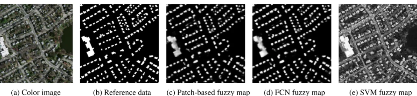
(a) Color image (b) Reference data (c) Patch-based fuzzy map (d) FCN fuzzy map (e) SVM fuzzy map
Fig. 2: Experimental results on a fragment of the Boston dataset. • Lower execution time at inference, given that
convolu-tions can enjoy the benefits of GPU processing. We convolutionalize the patch-based network depicted by Fig. 1. We choose an existing framework to benefit from a mature architecture and to carry out a rigorous comparison.
Fig. 1b depicts such conversion into a FCN. In the patch-based network, every output inside the output patch is located at a different position with respect to its so-called receptive field(the portion of the input to which it is connected). This behavior is hard to justify, so we will here pretend that the output patch is of size 1 × 1 instead of 16 × 16, thus just concentrating on a single centered output. We then rewrite the fully connected layer as a convolutional layer with one feature map and with the spatial dimensions of the previous layer (9 × 9). Finally, we add a deconvolutional layer that upsamples its input by a factor of 4, in order to recover the input resolution. Notice that the tasks of classification and upsampling are now separated.
This new network takes as input images of different sizes, with the output size varying accordingly. During the training stage, we emulate the learning as performed by the patch-based networks by taking an input of size 80 × 80 in order to produce maps of size 16 × 16 as before (see Fig. 1c). The input patch is larger than the one of patch-based networks, not because we are dealing with more context, but because every output is now centered in its context. At inference time we take inputs of arbitrary sizes to construct classification maps. For arbitrary size of input the FCN structure is always similar, with the same number of parameters.
Fig. 1c depicts the role of deconvolution: The output value of each neuron from the previous layer is multiplied by a learned filter, which is “pasted” in the output with a stride of 4. Overlapping occurs due to the size 8 × 8 of the filter. The overlapping areas are added (gray) while the excess ar-eas beyond border are excluded (white).
5. EXPERIMENTAL RESULTS
The CNNs were implemented using the Caffe deep learning framework [10]. In a first experiment we apply our approach to the Massachusetts Buildings Dataset [6]. The dataset con-sists of color images over Boston with 1m2spatial resolution,
covering an area of 340km2for training and 22.5km2for test-ing. The images are labeled into two-classes: building and non-building. A portion of an image with its corresponding reference is depicted in Figs. 2a-b.
We train the patch-based and fully convolutional net-works (Figs. 1a and 1c respectively) for 30k stochastic gra-dient descent iterations on randomly sampled patches, with mini-batches of size 64, a learning rate of 0.0001, momentum 0.9 and a weight regularization of 0.0002. The parameters and rationale for selecting them are detailed by Mnih [6].
To evaluate the accuracy of the classification we used two different measures: pixel-wise accuracy (proportion of cor-rectly classified pixels, obtained though binary classification of the output probabilities with threshold 0.5) and the area un-der the receiver operating characteristics (ROC) curve [11]. The latter measures the overall quality of the fuzzy maps, be-ing 1 the area value correspondbe-ing to an ideal classifier.
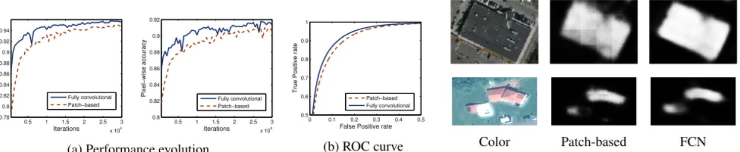
Fig. 3a plots the evolution of area under ROC curve and pixel-wise accuracy, through the iterations. The FCN consis-tently outperforms the patch-based network. Fig. 3b shows ROC curves for the final networks after training, the FCN ex-hibiting a better relation between true and false positive rates (areas under ROC curves are 0.9922 for FCN and 0.9899 for the patch-based network). Fig. 2c-d depicts visual fragments. To further evaluate the benefits of neural networks over other previous learning approaches we trained a support vec-tor machine (SVM) with Gaussian kernel on 1k randomly selected pixels of each class. Such SVM-based approach is common for remote sensing image classification [1].
As shown by Fig. 2e, such pixel-wise SVM classification often confuses roads with buildings as their colors are similar, while neural networks better infer and separate the classes by taking into account the geometry of the context. The accuracy on the Boston test dataset is 0.6229 and its area under ROC curve is 0.5193 (lower than with CNNs, as shown in Fig.3).
In terms of efficiency the FCN also outperforms the patch-based CNN. Instead of carrying out the prediction in a small patch basis, the input of the FCN is simply increased to output larger predictions, better benefiting from the GPU paralleliza-tion of convoluparalleliza-tions. The execuparalleliza-tion time to classify the whole Boston 22.5km2dataset (run on an Intel I7 CPU @ 2.7Ghz with a Quadro K3100M GPU) is 82.21s with the patch-based
0.5 1 1.5 2 2.5 3 x 10⁴ 0.78 0.8 0.82 0.84 0.86 0.88 0.9 0.92 0.94 Iterations
Area under ROC curve Fully convolutional Patch−based 0.5 1 1.5 2 2.5 3 x 10⁴ 0.8 0.82 0.84 0.86 0.88 0.9 0.92 Iterations
Pixel−wise accuracy Fully convolutional
Patch−based
(a) Performance evolution
0 0.1 0.2 0.3 0.4 0.5 0.5 0.6 0.7 0.8 0.9 1
False Positive rate
True Positive rate
Patch−based Fully convolutional
(b) ROC curve
Fig. 3: Evaluation on the Boston test set.
Color Patch-based FCN
Fig. 4: Border discontinuities are removed through the FCN (top: Boston, bottom: Forez).
(a) Color image (b) Fuzzy map (c) Binary map
Fig. 5: Classification of a Pleiades image, with an FCN.
CNN against 8.47s with the FCN, showing a 10x speed-up. In a second experiment we visually demonstrate the ef-fectiveness of FCNs for the classification of a Pleiades image covering the area of Forez, France, at a 0.5m2 spatial reso-lution. We use a pansharpened color version of the image, which we train for 30k iterations on patches extracted from a subset of the surface that covers 24.75km2. The classes and the parameters used for training are the same as for the Boston network. To preserve the amount of spatial context in this higher resolution image, we first subsample the image and then linearly upsample the output patches. The reference data used for training are extracted from OpenStreetMap project. Fig. 5 shows a test subset and its corresponding classification map. The time to infer a tile of 2.25km2is 10.6 seconds for a patch-based CNN and 1.8 for the FCN.
As shown in the amplified fragments from both images (Fig. 4), the border discontinuities present in the patch-based scheme are absent in our fully convolutional setting.
6. CONCLUDING REMARKS
This work addresses the problem of remote sensing image classification with convolutional neural networks. CNNs are mostly used to categorize images, hence new architectures must be designed for dense pixel-wise classification. To this end, we proposed a fully convolutional neural network. By imposing the restriction that all layers must be convolutional or deconvolutional, the learning process is enhanced and the execution time reduced. Our experimental results show that such networks outperform previous approaches both in accu-racy and in the computational time required for inference.
7. REFERENCES
[1] Y. Tarabalka, J.A. Benediktsson, and J. Chanussot, “Spectral-spatial classification of hyperspectral imagery based on partitional clustering techniques,” IEEE TGRS, vol. 47, no. 8, pp. 2973–2987, 2009.
[2] Yann LeCun, L´eon Bottou, Yoshua Bengio, and Patrick Haffner, “Gradient-based learning applied to document recognition,” Proceedings of the IEEE, vol. 86, no. 11, pp. 2278–2324, 1998.
[3] Tong Li, Junping Zhang, and Ye Zhang, “Classification of hyperspectral image based on deep belief networks,” in ICIP. IEEE, 2014, pp. 5132–5136.
[4] Yushi Chen, Xing Zhao, and Xiuping Jia, “Spectral-spatial classification of hyperspectral data based on deep belief network,” IEEE J-STARS, vol. 8, no. 6, June 2015. [5] Ot´avio AB Penatti, Keiller Nogueira, and Jefersson A dos Santos, “Do deep features generalize from everyday objects to remote sensing and aerial scenes domains?,” in IEEE CVPR Workshops, 2015, pp. 44–55.
[6] Volodymyr Mnih, Machine learning for aerial image labeling, Ph.D. thesis, University of Toronto, 2013. [7] Alex Krizhevsky, Ilya Sutskever, and Geoffrey E
Hin-ton, “Imagenet classification with deep convolutional neural networks,” in NIPS, 2012, pp. 1097–1105. [8] Christopher M Bishop, Neural networks for pattern
recognition, Oxford university press, 1995.
[9] Jonathan Long, Evan Shelhamer, and Trevor Darrell, “Fully convolutional networks for semantic segmenta-tion,” in CVPR, 2015.
[10] Yangqing Jia, Evan Shelhamer, Jeff Donahue, Sergey Karayev, Jonathan Long, Ross Girshick, Sergio Guadar-rama, and Trevor Darrell, “Caffe: Convolutional ar-chitecture for fast feature embedding,” arXiv preprint arXiv:1408.5093, 2014.
[11] C`esar Ferri, Jos´e Hern´andez-Orallo, and Peter A Flach, “A coherent interpretation of AUC as a measure of ag-gregated classification performance,” in ICML, 2011.