Classification by Opinion-Changing
Behavior: A Mixture Model Approach
Jennifer L. Hill
Department of Statistics, Harvard University, 1 Oxford St., Cambridge, MA 02138
e-mail: [email protected] Hanspeter Kriesi
Department of Political Science, University of Geneva, UNI-MAIL, 102 bd Carl-Vogt, CH-1211 Geneva 4, Switzerland
e-mail: [email protected]
We illustrate the use of a class of statistical models, finite mixture models, that can be used to allow for differences in model parameterizations across groups, even in the ab-sence of group labels. We also introduce a methodology for fitting these models, data augmentation. Neither finite mixture models nor data augmentation is routine in the world of political science methodology, but both are quite standard in the statistical literature. The techniques are applied to an investigation of the empirical support for a theory (devel-oped fully by Hill and Kriesi 2001) that extends Converse’s (1964) “black-and-white” model of response stability. Our model formulation enables us (1) to provide reliable estimates of the size of the two groups of individuals originally distinguished in this model, opinion holders and unstable opinion changers; (2) to examine the evidence for Converse’s basic claim that these unstable changers truly exhibit nonattitudes; and (3) to estimate the size of a newly defined group, durable changers, whose members exhibit more stable opinion change. Our application uses survey data collected at four time points over nearly 2 years which track Swiss citizens’ readiness to support pollution-reduction policies. The results, combined with flexible model checks, provide support for portions of Converse and Zaller’s (1992) theories on response instability and appear to weaken the measurement-error ar-guments of Achen (1975) and others. This paper concentrates on modeling issues and serves as a companion paper to Hill and Kriesi (2001), which uses the same data set and model but focuses more on the details of the opinion-changing behavior debate.
Authors’ note: Jennifer Hill is a postdoctoral fellow at Columbia University’s School of Social Work, 622 West
113th Street, New York, NY 10025. Hanspeter Kriesi is a Professor in the Department of Political Science, University of Geneva, UNI-MAIL, 102 bd Carl-Vogt, CH-1211 Geneva 4, Switzerland. The authors gratefully acknowledge funding for this project partially provided by the Swiss National Science Foundation (Project 5001-035302). Thanks are due to Donald Rubin for his help in the initial formulation of the model, as well as John Barnard, David van Dyk, Gary King, Jasjeet Sekhon, Andrew Gelman, Stephen Ansolabehere, and participants in Harvard University’s Center for Basic Research in the Social Sciences Research Workshop in Applied Statistics for helpful comments along the way. Klaus Scherer should be acknowledged for his role in organizing the first Swiss Summer School for the Social Sciences, where this collaborative effort was born. We would like to express our gratitude to three anonymous reviewers of this journal whose comments greatly contributed to the clarification of our argument.
Copyright 2001 by the Society for Political Methodology
1 Introduction
PREVIOUSLY (Hill and Kriesi 2001) we considered the debate among Converse (1964), Achen (1975), and Zaller (1992) regarding opinion stability by using a mixture model fit via data augmentation. In this paper we lay out the statistical foundations of that model as well as the estimation algorithm employed. We demonstrate how this approach allows us to build and fit a model specifically tailored to the political science questions of primary interest.
In 1964, Philip Converse put forth his “black-and-white” theory of opinion stability. He tested this theory using ad hoc methods and found support for this simple model with only one of the survey items he had at his disposal. This theory has yet to be tested using more sophisticated techniques and a more realistic version of the model.
In Converse’s black-and-white model, there are two groups of individuals—a perfectly stable group and a random group. We refer to these, respectively, as opinion holders and vacillating changers. We extend Converse’s model in a way that allows us to separate out a small but substantively important third group of individuals—those who make stable opinion changes—from those who appear to make more unstable changes (the vacillating changers). This distinction leads to a more refined profile of the unstable or “vacillating” changers that, in turn, yields a sharper estimate of their true percentage in the population and facilitates a more detailed examination of whether they truly seem to exhibit what Converse (1964) referred to as “non-attitudes.”
The methodological problem in fitting this model to survey data is that the true group classification for any given survey respondent is unknown. For example, although an indi-vidual may respond in a way that appears to be perfectly stable over time, she in fact may be doing so by chance and, thus, might still be a vacillating changer. Her responses provide us with information about which group classification appears more likely, but they do not determine this classification.
A finite mixture model (Everitt and Hand 1981; Titterington et al. 1985; Lindsay 1995) provides us with a straightforward mapping from our theoretical model that postulates three latent classes of people because it is specifically intended for this sort of situation where group labels are missing. We show how this model can be fit using a statistical algorithm known as data augmentation (Tanner and Wong 1987). We use flexible model checks in the form of posterior predictive checks and Bayes factors to compare competing models and test substantive hypotheses. The results provide empirical support for aspects of both Converse’s black-and-white model and Zaller’s (1992) notion of responder ambivalence. They provide evidence against the measurement-error explanation of response instability (e.g. see Achen 1975).1
2 Opinion-Changing Behavior 2.1 The Data
The data come from a Swiss study on pollution abatement policies. The issues involve regulation of the use of citizen’s cars and were publicly debated in Switzerland at the time of the study. Responses to questions regarding each of the following six policies were measured at four time points over 2 years (December 1993; Spring 1994; Summer 1994; Fall
1For a more detailed description of the placement of our argument within the context of this debate please see Hill and Kriesi (2001).
1995): speed limits, a tax on CO2(implying a price increase for gas of about 10centimes/L), a large price increase for gas (up to 2fr./L), promotion of electrical vehicles, car-free zones, and parking restrictions.
The first two waves have complete responses from 1062 respondents. However, there are missing data in the third and fourth time periods. Overall, complete data exist for 669 respondents; the missing data rates for each individual question are all approximately 37%. We use a complete-case approach for the current analyses. That is, for the analysis of each question we include only individuals who responded at all four time points. Theoretically, we should use a more principled approach to missing data (see, e.g., Little and Rubin 1987). However, separate work examining the implications of different missing data assumptions for this study demonstrates no strong departures from the substantive conclusions reached in this paper when models that accommodate missing data are used (Hill 2001).
The present analysis focuses on one question at a time. The coding we use in our analyses for the response Y for the i th individual at the t th time point is
Yt,i =
1 for “strongly disagree”
2 for “mildly disagree”
3 for “no opinion”
4 for “mildly agree”
5 for “strongly agree”
Despite the ordering presented here, we emphasize that our model does not necessitate conceptualization of the responses on an ordinal scale from strong agreement to strong disagreement (with or without allowing for the “no opinion” category to lie in the center of this ordinal ranking). This concept is discussed in greater detail in Section 2.2.
The bivariate correlations between our Swiss items display the same temporal pattern as that which led Converse to his black-and-white model in the first place, but they suggest a rather high level of stability: they are located in the range (.45 to .50) of the correlations for American social welfare items reported by Converse and Markus (1979) for the less constraining issues and in the range of the American moral issues (.62 to .64) for the more constraining issues2(for more detail see Hill and Kriesi 2001).
2.2 Building a Model
Our goal in building a model is elucidation of the empirical support for a specific theory about opinion-changing behavior (as well as some derivatives of this theory). Therefore we build a model that is specifically tailored to our political science theory. To do so we first clearly lay out the substantive theory we want to represent and then translate it into probability statements.
2.2.1 The Theory
We postulate the existence of three categories of people with regard to opinion-changing behavior: opinion holders, vacillating changers, and durable changers. Each of these groups
2Note, however, that the issue-specific stability observed for our Swiss policy measures still falls far short of the stability (.81 to .83) that has been measured in the United States for a basic political orientation such as one’s party identification.
behaves differently on average. Perhaps most importantly, we would expect the probabil-ity that an individual’s series of responses over time follows a particular type of pattern to vary across opinion-changing behavior groups. In addition, though, we might expect differences between groups with regard to other characteristics of interest. For instance, there is no reason to believe that members of different groups would have the same prob-ability of agreeing with a given issue. Strength of opinion is also likely to vary across groups.
Another general aspect of our theory is that we have no reason to believe that a “no opinion” response in any way represents a middle ground between agreeing with and dis-agreeing with an issue, as opposed to a distinct category. Such an ordering would force us to make a potentially strong assumption about how these categories are related.
Accordingly, there are four key elements to the model we would like to build. First, the model must include a different submodel for each opinion-changing group and each submodel should allow for different types of behaviors that distinguish the groups. Second, our model must accommodate the fact that group membership labels are not observed. Third, we would like to treat agreeing with an issue, holding no opinion about an issue, and disagreeing with an issue as distinct categories without forcing them to represent an ordering from one extreme to another with “no opinion” lying in the middle of the continuum. Fourth, and in keeping with our general goal of elucidating theory, model parameters should be readily interpretable in terms of the underlying political science construct.
2.2.2 Finite Mixture Models
Sometimes the data we observe are not all generated by the same process. Consider American citizens’ attitudes toward a tax cut or their rating of the current president’s performance. If we plot data measuring these attitudes (from a 7-point Likert scale, for instance), the distribution might appear bimodal, with a peak somewhere on each end of the spectrum. Such data can be conceptualized as belonging to a mixture of two distributions, each corresponding roughly to identification with one of the two major parties. If party membership were recorded, then each distribution could be modeled separately so that the unique aspects of each could be considered. Unfortunately, this class variable may itself be unobserved. If this is the case, we can represent this structure by a finite mixture model.
Formally, finite mixture distributions can be described by
p(x)= π1f1(x)+ · · · + πJfJ(x)= J
X
j=1 fj(x)
where the fj(x) can each represent different distributions (even belonging to different
families of distributions) relying, potentially, on entirely distinct parameters (Everitt and Hand 1981; Titterington et al. 1985; Lindsay 1995).
We use a finite mixture model to accommodate the first two of our key features. In our example, group membership is the unobserved class variable. Note how this model allows for specification of different submodels, fj(x), corresponding to different types of behavior,
for each opinion-changing group.
Unobserved categories are sometimes referred to as “latent classes.” The analysis we perform should therefore be distinguished from a set of methods commonly referred to as latent class analysis (McCutcheon 1987). Latent class analysis attempts to uncover latent structure in categorical data by identifying latent (unobserved) classes such that within each class the observed variables are independent of each other. Our model also postulates the existence of unobserved classes; however, these classes are defined by more complex
probabilistic structures than the “local independence” properties common to traditional models for latent class analysis.
2.2.3 Competing Off-the-Shelf Models and Desired Features Three and Four
There are several standard models and corresponding off-the-shelf software packages that can be used to “fit” longitudinal survey data. Time-series or panel data models, which postulate normal or ordered multinomial probit or logit models at each time point, represent one set of options. Alternatively a multinomial structure that allows for different probabilities for each pattern of responses (necessitating many constraints on the cell probabilities due to the sparseness of the data relative to the number of possible patterns) can be used.
Any of these methods could be subsumed within a finite mixture model, although model fitting would then require more sophisticated techniques. The standard models present difficulties with our third and fourth key elements, however. The time-series models do not represent a natural mapping from the parametric specification to the types of behavior in which we are interested. Moreover, they force an ordinal interpretation of the survey response categories.
The model we present in this paper is actually mathematically equivalent to a product multinomial model, where the group membership labels are treated as unknown parameters, and with a particular set of complicated constraints. We believe that our parameterization and its associated conceptual representation (see, for instance, the tree structure displayed in Fig. 1), however, constitute a far clearer mapping from the theoretical model to the probabilistic model. Therefore the parameters actually all have direct substantive meaning in terms of our theory regarding opinion-changing behavior. In addition our model does not necessitate an assumption of ordinal response categories.
2.3 Parameterization: The Full Model
Study participants are characterized as belonging to one of the three groups described briefly in Section 1 with regard to each policy measure for the duration of the study period. These qualifications are important: the labels used to describe people are policy issue and time period dependent. For instance, an individual could be a durable changer regarding the CO2 tax issue during the time period spanned by this study, however, he might well be an opinion holder regarding the same issue 10 years later. Similarly, an individual might be a durable changer with respect to the tax on CO2during this time period but an opinion holder with respect to speed limits during this time period.
If we denote the three-component vector random variable for group membership for the i th person as Gi = (g1,i, g2,i, g3,i), the probability of falling into each group can be described by the following parameters:
π1 = Pr(individual i belongs to opinion-holder group) = Pr(Gi = v1) π2 = Pr(individual i belongs to vacillating-changer group) = Pr(Gi = v2) π3 = Pr(individual i belongs to durable-changer group) = Pr(Gi = v3)
whereπ1+π2+π3= 1, and the vjare simply vectors of length 3 with a 1 in the j th position
and 0 elsewhere. These are the parameters of primary interest; the rest of the parameters, described in the following three sections, are used to characterize the response behavior of each of the three groups. A fuller, more intuitive description of these submodels is given by Hill and Kriesi (2001).
2.3.1 Opinion Holders
Opinion holders are defined as those who maintain an opinion either for or against an issue. Anyone who responded with a “no opinion” at any time point cannot be in this group, nor can anyone who crossed an “opinion boundary” across time points (i.e., an opinion holder cannot switch from an agree response to a disagree response, or vice versa).
Two parameters,
α1= Pr(Y1,i = 1 or 2 | Gi = v1) and
δ1= Pr(Yt,i = 1 | Y1,i ∈ {1, 2}, Gi = v1)= Pr(Yt,i = 5 | Y1,i ∈ {4, 5}, Gi= v1) are used to describe the behavior of opinion holders across the four time points, given the constraints
Pr(Yt,i = 3 | Gi= v1)= 0, ∀t Pr(Yt,i ∈ {3, 4, 5} | Y1,i ∈ {1, 2}, Gi= v1)= 0, ∀t 6= 1 Pr(Yt,i ∈ {1, 2, 3} | Y1,i ∈ {4, 5}, Gi= v1)= 0, ∀t 6= 1
which formally set
1− α1 = Pr(Y1,i = 4 or 5 | Gi = v1)
1− δ1 = Pr(Yt,i = 2 | Y1,i ∈ {1, 2}, Gi = v1)= Pr(Yt,i = 4 | Y1,i ∈ {4, 5}, Gi = v1) These parameters allow for differing probabilities of being for or against an issue and, conditional on being for or against an issue, differing probabilities of feeling strongly or mildly about it. Note that for parsimony the parameter for the extremity or strength3of the reaction (δ1) does not vary across time periods or across opinions (agree or disagree), even though this may not be the most accurate representation of reality.
2.3.2 Vacillating Changers
For the purposes of this model, we again make a simplifying assumption: the members of the group we label vacillating changers do not change their opinions in any particularly systematic way. Moreover, the responses of the members of this group are considered to be independent across time points. Therefore any pattern of responses could characterize a vacillating changer, for a total of 625 possible response patterns.
On the basis of this assumption, the behavior of a vacillating changer at any time point can be characterized by three parameters:
ϕ2 = Pr(Yt,i = 3 | Gi = v2) α2 = Pr(Yt,i ⊂ {1, 2} | Gi = v2)
δ2 = Pr(Yt,i = 1 | Yt,i ⊂ {1, 2}, Gi = v2)= Pr(Yt,i = 5 | Yt,i ⊂ {4, 5}, Gi = v2) 3Extremity is one of many indicators of opinion or attitude strength (see Krosnick and Fabrigar 1995).
Our model does allow vacillating changers to have some minimal structure in their re-sponses. They are allowed different probabilities (constant over time) for having no opinion, agreeing, or disagreeing. The model also allows them to have different probabilities (con-stant over time) for extreme versus mild responses, given that they express an opinion. The fact that our model postulates that the probability to agree can be different from the probability to disagree is contrary to Converse’s black-and-white model, which assumes that the probability that a vacillating changer agrees with an issue is equal to the probability that he disagrees with the issue:
1− ϕ2
2 = α2= 1 − ϕ2− α2
This constraint reflects Converse’s notion of “non-attitudes” among unstable opinion chang-ers and will be tested in Section 5.
2.3.3 Durable Changers
Durable changers are defined as those who change their opinion or who form an opinion based on some rational decision-making process perhaps prompted by additional infor-mation or further consideration of an issue. Durable changers are allowed to change their opinion (e.g. from mildly disagreeing to strongly agreeing) exactly once across the four time periods. This characteristic distinguishes them from the vacillating changers that are allowed to move back and forth freely. In contrast to vacillating changers, durable changers adopt a new, stable opinion, either by changing sides or by forming an opinion for the first time. They are not allowed to change to the “no opinion” position, but they can move out of this position. This implies that those switching from a for position must switch to an against position, and vice versa.
It is arguable that a reasonable relaxation of this model would be to allow individuals to change from a given opinion (strong or weak), to the “no opinion” category, and then to the opposite opinion (strong or weak). Empirically we find that this pattern does not happen too often (once for speed limits and car free zones, five times for gas price increase and parking restrictions, eight times for CO2tax and electric vehicles). Even if all such individuals were allocated to the durable-changers category for the questions with the highest incidence of them, it would increase the average proportion of durable changers by just slightly over one percent. Therefore, we are not overly concerned about the impact of this possible model oversimplification on our inferences.
Since the durable-changers group comprises only individuals who switch exactly once across the four time periods, the parametric descriptions of their behavior revolve primarily around descriptions of this opinion switch. Only one parameter is specified for post-switch behavior, the probability that someone who starts with no opinion switches to a disagree response, α(post) 3 = Pr ¡ Y(ti∗+1),i ∈ {1, 2} | Yti∗= 3, Gi = v3 ¢
where ti∗represents the time period directly prior to a change in opinion. This simplicity is achieved because we do not differentiate this behavior by switching time and switches to no opinion are not allowed.
However, in parametrizing the opinions that the durable changers switch away from, we distinguish between leaving an opinion category and leaving the “no opinion” position. This is the distinction between durably changing an opinion and forming a durable opinion
for the first time. Moreover, we allow the direction of change to differ between the first period, on the one hand, and the second and third period, on the other hand. Since durable changers are assumed to be strongly influenced by the additional information which they receive, the direction of their change is a function of the “tone” of the public debate. Four parameters define the probabilities for these options:
ϕ(pre1) 3 = Pr ¡ Yti∗,i = 3 | ti∗ = 1, Gi = v3 ¢ ϕ(pre2) 3 = Pr ¡ Yti∗,i = 3 | ti∗ ∈ {2, 3}, Gi = v3 ¢ α(pre1) 3 = Pr ¡ Yti∗,i ∈ {1, 2} | ti∗= 1, Gi = v3 ¢ α(pre2) 3 = Pr ¡ Yti∗,i ∈ {1, 2} | ti∗∈ {2, 3}, Gi= v3 ¢
Accounting for panel or “Socratic” effects (McGuire 1960; Jagodzinski et al. 1987; Saris and van den Putte 1987), which typically occur between the first two waves of a panel study, we distinguish between the probability that an opinion change occurs after the first period and the probability that it occurs after the second or third period (these last two are set equal to each other). This is captured by
τ3 = Pr(ti∗= 1 | Gi= v3) 1− τ3
2 = Pr(t ∗
i = 2) = Pr(ti∗= 3)
Note the constraint that
Pr¡Y(ti∗+1),i = 3 ¢
= 0
Finally, as we did for the other two groups, we again allow for a stable share of strong opinions:
δ3= Pr(Yt,i = 1 | Yt,i ∈ {1, 2}, Gi = v3) = Pr(Yt,i = 5 | Yt,i ∈ {4, 5}, Gi = v3)
2.4 The Model as a Tree
It is helpful to think of the finite mixture model reflecting the behavior of these three groups as being represented by a tree structure such as the one illustrated in Fig. 1. This tree slightly oversimplifies the representation of our model (the vacillating-changer branch of the tree, for instance, represents the response for just one given time period). However, it does reflect the types of behavior that are pertinent for defining each group.
This model is an example of a finite mixture model because it can be conceived as a mixture of three separate models where the mixing proportions are unknown. In this case the full model is a mixture of the models for each opinion-changing behavior group because, in general, we cannot deterministically separate one group from the next since the members of the different groups cannot be identified as such. Our model will be better behaved than some mixture models, however, because of the structure placed on the behavior of each group. In particular, individuals who cross opinion boundaries more than once can only
Fig. 1 T ree structure of the model.
be members of the vacillating-changers group. This identification creates a nonsymmetric parameter space which prevents label-switching in the algorithm used to fit this model. Recent examples of fully Bayesian analyses of mixture model applications include Gelman and King (1990), Turner and West (1993), and Belin and Rubin (1995).
2.5 The Likelihood
We derive the likelihood in a slightly roundabout fashion to make explicit the connection between our model and the product multinomial model discussed briefly in the beginning of Section 2.2. There are 625 response patterns possible in the data. Therefore a simple model for the observed data is a multinomial distribution where each person has a certain probability of falling into each of 625 response-pattern bins. However, this model would ignore the group structure in which we are most interested. An extension of this idea to a model for the complete data which includes not only the response patterns, X , but also the group membership indicators, G, would be a product multinomial model with a separate multinomial model for each group.
Let Xidenote a vector random variable of length 625 with elements Xk,i, where Xk,i = 1
if individual i has response pattern k and 0 otherwise. If the group membership of each study participant were known, the likelihood function would be
L(θ | X, G) = N Y i=1 625 Y k=1 3 Y j=1 (πjpk· j)xk,igj,i
whereθ represents the model parameters, and pk· j denotes the probability4 of belong-ing to cell k (havbelong-ing response pattern k) given that one is in group j . This is called the “complete-data likelihood” because it ignores the missingness of the group membership labels.
The likelihood function given only the observed data (which does not include the group membership labels), however, is
L(θ | X) = N Y i=1 L(θ | Xi) = N Y i=1 X Gi∈3 L(θ | Xi, Gi) = N Y i=1 X Gi∈3 625 Y k=1 3 Y j=1 (πjpk· j)xk,igj,i = N Y i=1 X Gi∈3 625 Y k=1 (π1pk.1)xk,ig1,i(π2pk.2)xk,ig2,i(π3pk.3)xk,ig3,i = N Y i=1 µ π1 625 Y k=1 pxk.i k.1+ π2 625 Y k=1 pxk.i k.2+ π3 625 Y k=1 pxk.i k.3 ¶ (1)
where3 = {(1, 0, 0), (0, 1, 0), (0, 0, 1)}, the sample space for Gifor all i .
4Note that although many of the p
k· jare structural zeros, the corresponding xk,igj,iwill always be zero as well,
Maximum-likelihood estimation, which requires us to maximize Eq. (1) as a function of θ, is complicated by the summation in this expression. In addition, we have nowhere near enough data to estimate all the parameters in this more general model, nor would these estimates be particularly meaningful for political science theory without some further structure. Clearly some constraints need to be put on these 1875 cell probabilities.
2.6 Reexpressing the Data
The tree structure described in Section 2.4, however, illustrates exactly the types of be-havior that we are most interested in and, consequently, the types of bebe-havior we need to measure. Rather than defining a survey respondent by her response pattern (and corre-sponding multinomial cell), for example, “1255,” we need to characterize her in terms of a limited number of more general variables, which allow us to reproduce her trajectory, e.g., as someone who started out opposed to the issue (first extremely, “1,” then not, “2”) and then crossed an opinion boundary and expressed strong agreement with the issue, “55.” Therefore all of the data have been reexpressed in terms of the variables described below. These variables, along with group indicators, define the elements which are used in the parameter estimates. That is, since the model parameters represent the probabilities of cer-tain types of behavior, the transformed data measure the incidences of these same types of behavior.
Ai =
(
1 if the i th person’s initial response is a 4 or 5
0 otherwise
Bi = number of the ith individual’s responses that are either 1 or 5 across all t Ci = number of the ith individual’s responses that are 3
Di = number of times the ith individual crosses an opinion boundary Ei = ½ 0 if Di 6= 1 ti∗ otherwise Fi = (
0 if the i th individual’s preswitch response is a 1, 2, or 3, orDi 6= 1
1 if the i th individual’s preswitch response is a 4 or 5
Hi =
(
0 if the i th individual’s preswitch response is a 1, 2, 4, or 5, orDi 6= 1
1 if the i th individual’s preswitch response is a 3
Mi =
(
0 if the i th individual’s postswitch response is a 1, 2, or 3, orDi6= 1
1 if the i th individual’s postswitch response is a 4 or 5
Qi =
(
0 if the i th individual’s postswitch response is a 1, 2, 4, or 5, orDi6= 1
1 if the i th individual’s postswitch response is a 3
Ri = number of the ith individual’s responses that are either 1 or 2 across all t
2.7 Reexpression of the Likelihood
Using the new variables described in Section 2.6 (and for the reasons described in Section 2.2), we can reexpress the complete-data likelihood as
L(θ|Z, G) = N Y i=1 3 Y j=1 πgj,i j p z j,z gj,i
where pzj,iis the probability that individual i belongs to group j conditional on his observed data, Zi.
The conditional probability of individual i being an opinion holder ( j = 1) given her responses (Zi) can be calculated as
p1z,i =¡α1−Ai
1 (1− α1)Ai(1− δ1)(4−Bi)δ1Bi ¢
∗ I(Ci = 0)I(Di = 0)
where I(·) is an indicator function which equals 1 if the condition in parentheses holds and equals 0 otherwise. The indicator functions constrain this probability to be zero for behavior that is disallowed for this group: responding with no opinion during at least one time period, I(Ci > 0); and, switching opinions, I(Di 6= 0).
Similarly, the conditional probability of belonging to each of the other groups given the observed responses can be expressed by the functions
pz2,i = ϕCi 2 α Ri 2 (1− ϕ2− α2)(4−Ci−Ri)δBi(1− δ2)(4−Ci−Bi) pz3,i = · τI(Ei =1) 3 (1− τ3) 2 I(I Ei ∈{2,3})³ ϕ(pre1)Hi 3 α
(pre1)(1−Fi )(1−Hi )
3
¡
1− α3(pre1)− ϕ3(pre1)¢Fi´I(Ei =1) ׳ϕ(pre2)Hi
3 α
(pre2)(1−Fi )(1−Hi )
3
¡
1− ϕ3(pre2)− α(pre2)3 ¢Fi´I(Ei ∈{2,3}) × ³¡1− α(post)3 ¢Mi¡α(post)3 ¢(1−Mi) ´Hi δBi 3 (1− δ3)(4−Bi−Ci) ¸ I(Di = 1)I(Qi = 0)
Clearly this model formulation ignores potentially relevant background information such as gender, age, political affiliation, and income. Later efforts will incorporate this informa-tion in more complicated models.
3 Fitting the Model: EM and Data Augmentation
This section describes the algorithms that were used to fit this model. There is no off-the-shelf software for this particular model. However, the general algorithms presented are straight-forward and accepted as standard practice within Statistics. Programming was performed in S-plus (though virtually any programming language potentially could have been used).5The first algorithm discussed, EM, can be used to find maximum-likelihood estimates for each parameter. This is helpful, but not fully satisfactory, if we are also concerned with our un-certainty about the parameter values. The data augmentation algorithm estimates the entire distribution (given the data) for each parameter in our model.
5In particular, any package that allows the user to draw from multinomial distributions and gamma distributions (which in turn can be converted to draws from beta and Dirichlet distributions) can be used.
3.1 A Maximum-Likelihood Algorithm—EM
The problem with using our model to make inferences is that it relies on knowledge of group membership, which, in practice, we do not have. The EM algorithm is a method which can be used to compute maximum-likelihood estimates in the presence of missing data. It is able to sidestep the fact that we do not have group membership indicators by focusing on the fact that if we had observed these “missing” data, the problem would be simple. It is an iterative algorithm with two steps: one that “fills in” the missing data, the
E-step (expectation step); and one that estimates parameters using both the observed and
the filled-in data, the M-step (maximization step). EM has the desirable quality that the value of the observed-data log-likelihood increases at every step.
We iterate between the two steps until an accepted definition of convergence is reached. In our case, iterations continued until the log-likelihood increased by less than 1× 10⁻¹⁰. Starting values of parameters for the first iteration were chosen at random. Checks were performed to ensure that the same maximum-likelihood estimates for each model were reached given a wide variety (100) of randomly chosen starting values; this helps to rule out multimodality of the likelihood.
3.1.1 The E-Step
The E-step for this model replaces the missing data with their expected values. Specifically, we take the expected value of the complete-data log likelihood,`,
Q= E£`(θ | Z, G) | Z, θ¤
where the expectation is taken over the distribution of the missing data, conditional on the observed data, Zi, and the parameters from the previous iteration of the M-step,
p¡Gi| Zi, θ ¢ = 3 Y j=1 Ã πjpzj,i P3 j=1πjpzj,i !gj,i
Q is linear in the missing data (the group indicators), so the E-step reduces to finding the
expectation of the missing data and plugging it into the complete-data log likelihood. The expectation of the indicator for group j and individual i is
E£Gi = vj| Zi, θ ¤ = πjp z j,i P3 j=1πjpzj,i
which is the probability, given individual i ’s response pattern, of falling into group j relative to the other groups.
3.1.2 The M-Step
The M-step finds maximum-likelihood estimates for all of our parameters. All of these parameter estimates are quite intuitive. For instance, the estimate forϕ2is
ˆ
ϕ2= PN
i=1g2,iCi
4T2
where T2 is the sum of the individual-specific weights, g2,i (calculated in the E-step), corresponding to the vacillating-changers group. This estimate takes the weighted sum of “no opinion” responses (Ci) across the four time periods (where each weight reflects
the probability that the person is a vacillating changer) and divides it by the number of people we expect to belong to this group (the sum of the weights, T2) multiplied by four (for the four time periods; four possible responses for each person). This is the logical estimate for the parameters representing the probability that a vacillating changer will respond with “no opinion” at any given time point.
The following are the equations for the entire set of parameter estimates that maximize
Q given the estimates of Gi = (g1,i, g2,i, g3,i) from the E-step (where Tj =
PN i=1gj,i): ˆ πj = Tj P3 j=1Tj , j= 1, 2, 3 ˆ α1 = PN i=1g1,iI(Ci = 0)I(Di = 0)(1 − Ai) PN i=1g1,iI(Ci = 0)I(Di= 0) ˆ δ1 = PN i=1g1,iI(Ci = 0)I(Di = 0)Bi 4PNi=1g1,iI(Ci = 0)I(Di = 0) ˆ ϕ2 = PN i=1g2,iCi 4T2 ˆ α2 = PN i=1g2,iRi 4T2 ˆ δ2 = PN i=1g2,iBi PN i=1g2,i(4− Ci) ˆ ϕ(pre1) 3 = PN
i=1g3,iI(Ei= 1)I(Di = 1)I(Qi = 0)Hi
PN
i=1g3,iI(Ei= 1)I(Qi = 0)I(Di = 1)
ˆ
α(pre1)
3 =
PN
i=1g3,iI(Ei= 1)I(Di = 1)I(Qi = 0)(1 − Fi)(1− Hi)
PN
i=1g3,iI(Ei = 1)I(Di = 1)I(Qi = 0)
ˆ
ϕ(pre2)
3 =
PN
i=1g3,iI(Ei∈ {2, 3})I(Di = 1)I(Qi = 0)Hi
PN
i=1g3,iI(Ei∈ {2, 3})I(Di = 1)I(Qi = 0)
ˆ
α(pre2)
3 =
PN
i=1g3,iI(Ei∈ {2, 3})I(Di = 1)I(Qi = 0)(1 − Fi)(1− Hi)
PN
i=1g3,iI(Ei ∈ {2, 3})I(Di = 1)I(Qi= 0)
ˆ α(post) 3 = PN i=1g3,iHiI(Di = 1)I(Qi= 0)(1 − Mi) PN i=1g3,iHiI(Di = 1)I(Qi= 0) ˆ δ3 = PN i=1g3,iI(Di = 1)I(Qi = 0)Bi PN i=1g3,iI(Di = 1)I(Qi = 0)(4 − Ci)
ˆ
τ3 = PN
i=1g3,iI(Di = 1)I(Qi = 0)I(Ei = 1)
PN
i=1g3,iI(Di= 1)I(Qi = 0)
3.2 The Data Augmentation Algorithm
While point estimates of the parameters are helpful, they are insufficient to answer all the questions we might have about the parameters. For instance, it is useful to understand how much uncertainty there is about the parameter estimate. One way to do this is to estimate the entire distribution of each parameter given the data we have observed; this distribution is called the posterior distribution. Posterior distributions formally combine the distribution of the data given unknown parameter values with a prior distribution on the parameters. This prior distribution quantifies our beliefs about the parameter values before we see any data. The priors used in this analysis reflect our lack of a priori information about the parameter values and are thus relatively “noninformative” (as discussed in greater detail later in this section).
The goal of the DA algorithm is to get draws from the posterior distribution p(θ | Z). It has two basic steps in this problem:
1. Draw the “missing data,” group membership indicators, given the parameters. 2. Draw the parameters, θ = (π1, π2, π3, α1, δ1, . . .), given the group membership
indicators.
3.2.1 Drawing Group Indicators Given Parameters
We can use the observed data for a given person along with parameter values to determine the probability that he falls in each group simply by plugging these values into the models we have specified for each group.6Then we can use these probabilities to temporarily (i.e., for one iteration) classify people into groups. For each person we sample from a trinomial distribution of sample size 1 with probabilities equal to (draws of ) the relative probabilities of belonging to each group (given individual characteristics):
p¡Gi| θ, Zi ¢ = Mult à π1p1z,i P3 j=1πjpzj,i , π2p z 2,i P3 j=1πjp z j,i , π3p z 3,i P3 j=1πjpzj,i !
These draws specify group membership labels.
3.2.2 Drawing Parameters Given Group Indicators
We sample parameters from their distribution conditioning on the data (i.e., using the infor-mation we have about our survey participants through their response behavior as measured by Z ) and the group indicators we drew in the previous step. This is akin to fitting a separate model for each group using only those people classified in the previous step to that group for each analysis.
6We obtain parameter values from the second step in each iteration, so for the first iteration we just start at a random place in the parameter space.
The posterior distribution can be expressed as p(θ | Z, G) = L(θ | Z, G)p(θ), where
p(θ) is the prior distribution on the parameters, θ. The complete data likelihood, L(θ | Z, G),
can be expressed as L(θ | Z, G) = N Y i=1 3 Y j=1 πgj,i j p z j,i gj,i = N Y i=1 π1g1,i ¡£ α(1−Ai) 1 (1− α1)Ai(1− δ1)(4−Bi)δ1Bi ¤ (I(Ci = 0)I(Di= 0)) ¢g1.i × π2g2,i ¡ ϕCi 2 α Ri 2 (1− ϕ2− α2)(4−Ci−Ri)δ2Bi(1− δ2)(4−Ci−Bi) ¢g2,i × π3g3,i ½· τI(Ei =1) 3 (1− τ3)I(Ei∈{2,3}) 2 ׳ϕ(pre1)Hi 3 α
(prel)(1−Fi )(1−Hi )
3
¡
1− α3(pre1)− ϕ3(pre1)¢Fi´I(Ei=1) ׳ϕ(pre2)Hi
3 α
(pre2)(1−Fi )(1−Hi )
3
¡
1− ϕ(pre2)3 − α3(pre2)¢Fi´I(Ei∈{2,3}) ׳¡1− α3(post)¢Mi¡α(post) 3 ¢(1−Mi)´Hiδ 3Bi(1− δ3)(4−Bi−Ci) ¸ × I(Di = 1)I(Qi = 0) ¾g3,i
We use Beta and Dirichlet distributions for our prior distributions. A Beta distribution is commonly used when modeling a probability or percentage because a Beta random vari-able is constrained to lie between 0 and 1. The mean of a Beta (a, b) is a/b. Therefore, the greater a is relative to b, the more the mass of the distribution is located to the left of .5, and vice versa. The variance of the distribution is ab/(a + b)2(a+ b + 1). There-fore the bigger the values of the parameters, the smaller the variance, and the tighter the distribution is about its mean. The Beta (1, 1) distribution is equivalent to a uniform dis-tribution from 0 to 1. The Dirichlet disdis-tribution is just the multivariate extension of the Beta distribution. The Dirichlet distribution with k parameters acts as a distribution for
k probabilities (or percentages) that all sum to 1 (such as is the case for the parameters
of a multinomial distribution). The Beta distribution is the conjugate prior7 for the bi-nomial distribution; the Dirichlet distribution is the conjugate prior for the multibi-nomial distribution.
If we assume a priori independence of appropriate parameters, we can factor p(θ) into six independent Beta distributions (forα1, δ1, δ2, τ3, α
(post)
3 , andδ3) and four independent Dirichlet distributions [for (π1, π2, π3), (ϕ2, α2, (1−ϕ2−α2)), (ϕ
(pre1) 3 , α (pre1) 3 , (1−ϕ (pre1) 3 − α(pre1) 3 )), and (ϕ (pre2) 3 , α (pre2) 3 , (1 − ϕ (pre2) 3 − α (pre2)
3 ))]. Parameters can then be drawn from the appropriate posterior distributions (found by standard conditional probability calculations). For example, if p(α1, 1 − α1) is specified as a Beta (a, b), then we would draw α (and (1− α)) from Beta [(a + N −PNi=1Ai), (b +
PN i=1Ai)].
7A conjugate prior is a prior that, when combined with a likelihood, yields a posterior distribution in the same family as itself. A Beta is conjugate to a binomial likelihood because the resulting posterior distribution is again Beta. Conjugate priors are generally the easiest to work with computationally.
Given the tree structure of the model and the conditional independence that it implies, prior independence of the parameters does not seem an unwarranted assumption. Priors were chosen to be as noninformative as possible. Beta and Dirichlet priors can be con-ceptualized as “pseudo-counts.” For instance, using a Beta (1, 1) prior for the distribution ofα1 can be thought of as adding one person to the group of opinion holders who were against the issue and one person to the group of opinion holders who were for the issue. The prior specifications used in these analyses give equal weight a priori to both (or all three) possibilities modeled by a particular distribution and keep the hyperparameters (pa-rameters of the priors) quite small. The primary prior used in this analysis is one which adds two “pseudo-people” to each opinion-changing behavior group (opinion holders, vac-illating changers, durable changers)—this is a Dirichlet distribution with parameters all equaling two—and then divides these people up evenly among the remaining categories. For instance, one person is allocated to agree and one person to disagree with the issue for opinion holders [a Beta (1, 1)]. The alternative priors tested uses this same idea but one starts with one person per opinion-changing group and the other starts with four people in each. Parameter estimates for the posterior distribution do not change meaningfully across priors.
3.2.3 Convergence
Iterations continue until we converge to a stationary distribution. Convergence can be as-sessed using a variety of diagnostics. We used the ˆR statistic proposed by Gelman and Rubin
(1992) and its multivariate extension discussed by Brooks and Gelman (1998). These di-agnostics monitor the mixing behavior of several chains, each originating from a different starting point. Then as many draws as are desired to estimate the empirical distribution sufficiently are taken. We used five chains, each with 2500 iterations, with the first 500 iterations treated as burn-in and discarded.
3.2.4 Superiority of the DA Algorithm
The DA algorithm was used in this problem because non-Bayesian techniques have generally been found to be flawed when applied to mixture models, particularly when calculating standard errors. In addition, the approximations which have been derived to accommodate testing of certain hypotheses are rather limited (see, e.g., Titterington et al. 1985) and cannot approach the flexibility in the types of inferences that can be performed trivially once we can sample from the posterior distribution (for a discussion, see van Dyk and Protassov 1999). Assuming that the correct model is used, the DA algorithm will converge to the correct posterior distribution. The properties exhibited in our simulations lead us to believe that our DA algorithms had converged well before we started saving draws from the posterior distribution.
4 Results
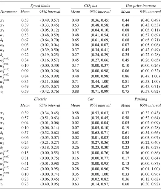
In this section we report the results of the model fit via the DA algorithm for each of the different policy measures. Table 1 presents the point estimate of the mean for each parameter as well as a 95% interval from the empirical posterior distribution (each with 10,000 draws). For all questions we see evidence for the existence of the durable-changer group (π3). The majority of people do seem to be either opinion holders or vacillating changers, however. Note that the vacillating changers, to varying degrees across question, appear to exhibit
Table 1 Estimate of parameters and their uncertainty for the unconstrained modela
Speed limits CO2tax Gas price increase
Parameter Mean 95% interval Mean 95% interval Mean 95% interval
π1 0.53 (0.49, 0.57) 0.40 (0.36, 0.45) 0.44 (0.40, 0.49) π2 0.39 (0.33, 0.45) 0.53 (0.48, 0.58) 0.48 (0.43, 0.53) π3 0.08 (0.05, 0.12) 0.07 (0.04, 0.10) 0.08 (0.05, 0.11) α1 0.53 (0.48, 0.59) 0.48 (0.41, 0.54) 0.63 (0.57, 0.69) δ1 0.67 (0.64, 0.70) 0.65 (0.61, 0.69) 0.68 (0.65, 0.71) ϕ2 0.03 (0.02, 0.04) 0.06 (0.04, 0.07) 0.07 (0.05, 0.08) α2 0.45 (0.39, 0.50) 0.37 (0.34, 0.41) 0.45 (0.42, 0.49) δ2 0.22 (0.19, 0.25) 0.27 (0.24, 0.29) 0.25 (0.22, 0.28) ϕ(pre1) 3 0.34 (0.16, 0.57) 0.45 (0.27, 0.66) 0.45 (0.26, 0.65) α(pre1) 3 0.10 (0.00, 0.30) 0.17 (0.00, 0.37) 0.10 (0.00, 0.26) ϕ(pre2) 3 0.09 (0.00, 0.26) 0.36 (0.00, 0.98) 0.06 (0.00, 0.32) α(pre2) 3 0.84 (0.56, 0.99) 0.48 (0.00, 0.98) 0.86 (0.47, 1.00) α(post) 3 0.35 (0.11, 0.66) 0.71 (0.44, 1.00) 0.81 (0.53, 1.00) δ3 0.49 (0.35, 0.67) 0.50 (0.39, 0.60) 0.57 (0.43, 0.71) τ3 0.59 (0.42, 0.76) 0.88 (0.71, 0.99) 0.75 (0.57, 0.92)
Electric Car Parking
Mean 95% interval Mean 95% interval Mean 95% interval
π1 0.39 (0.34, 0.45) 0.58 (0.53, 0.63) 0.37 (0.32, 0.43) π2 0.57 (0.51, 0.63) 0.40 (0.35, 0.45) 0.58 (0.52, 0.64) π3 0.04 (0.01, 0.06) 0.02 (0.00, 0.04) 0.05 (0.02, 0.09) α1 0.10 (0.06, 0.14) 0.07 (0.05, 0.10) 0.19 (0.08, 0.28) δ1 0.57 (0.52, 0.62) 0.68 (0.65, 0.71) 0.61 (0.54, 0.66) ϕ2 0.06 (0.05, 0.07) 0.02 (0.01, 0.03) 0.04 (0.03, 0.07) α2 0.24 (0.21, 0.27) 0.31 (0.27, 0.36) 0.33 (0.22, 0.40) δ2 0.20 (0.18, 0.23) 0.26 (0.23, 0.30) 0.23 (0.19, 0.27) ϕ(pre1) 3 0.15 (0.00, 0.55) 0.15 (0.00, 0.76) 0.36 (0.00, 0.86) α(pre1) 3 0.31 (0.00, 0.75) 0.16 (0.00, 0.77) 0.17 (0.00, 0.64) ϕ(pre2) 3 0.41 (0.01, 0.98) 0.25 (0.00, 0.95) 0.13 (0.00, 0.87) α(pre2) 3 0.47 (0.00, 0.95) 0.28 (0.00, 0.96) 0.79 (0.01, 1.00) α(post) 3 0.10 (0.00, 0.74) 0.35 (0.00, 1.00) 0.33 (0.00, 0.96) δ3 0.23 (0.06, 0.45) 0.37 (0.02, 0.82) 0.36 (0.12, 0.62) τ3 0.73 (0.40, 0.95) 0.63 (0.14, 0.97) 0.60 (0.30, 0.92)
aNotational convention is as follows. Subscripts: 1= opinion holders; 2 = vacillating changers; 3 = durable changers. Superscripts: pre1= opinion before a switch occuring after wave 1; pre 2 = opinion before a switch occuring after wave 2 or 3; post= opinion after a switch. Greek letters: π = group membership; α = disagree;
ϕ = no opinion; δ = extreme; τ = switched after 1st time period.
slight preferences with regard to the issues at hand. In particular, the estimate of the mean ofα2for the nonconstraining questions (electric, car, parking) appears to have been affected by the near-consensus views of the opinion holders with regard to these issues.
Note also that some of the intervals are very large, indicating a very low precision of some of the parameter estimates. This reflects our uncertainty regarding some of these parameters caused by a lack of a sufficient number of people who engaged in the types of behaviors to which these parameters correspond.
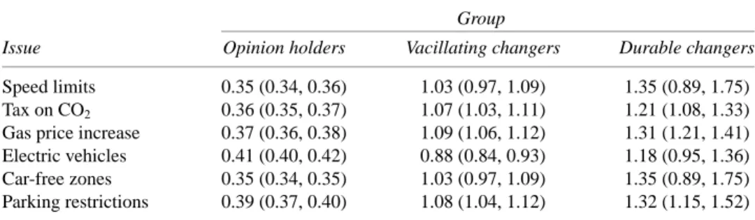
Table 2 Differences in average individual-level response variability across groups
Group
Issue Opinion holders Vacillating changers Durable changers
Speed limits 0.35 (0.34, 0.36) 1.03 (0.97, 1.09) 1.35 (0.89, 1.75)
Tax on CO2 0.36 (0.35, 0.37) 1.07 (1.03, 1.11) 1.21 (1.08, 1.33)
Gas price increase 0.37 (0.36, 0.38) 1.09 (1.06, 1.12) 1.31 (1.21, 1.41)
Electric vehicles 0.41 (0.40, 0.42) 0.88 (0.84, 0.93) 1.18 (0.95, 1.36)
Car-free zones 0.35 (0.34, 0.35) 1.03 (0.97, 1.09) 1.35 (0.89, 1.75)
Parking restrictions 0.39 (0.37, 0.40) 1.08 (1.04, 1.12) 1.32 (1.15, 1.52)
4.1 Evidence for the Measurement-Error Explanation of Response Instability
We would also like to use our model to explore the evidence for or against the measurement-error interpretation of response instability.
To do this we calculate the posterior distribution of the average individual-level standard deviation in responses for each group p(¯s( j ), | Y, G), j = 1, 2, 3, where,
¯s( j )= 1 Tj X i∈{i:Gi=vj} si and where si = q 1 3(Yi− ¯Yi)2 and ¯Yi = 1 4 P
tYt,i. These calculations treat the survey
responses as ordinal (using the ordering displayed in Section 2.1) just as the measurement error models do. If the response variability looks fairly similar (i.e., as if they came from the same distribution) across groups, then we might not mind labeling this variability simply as unexplained variation or measurement error.
Table 2 presents the means for each of these distributions; 95% intervals are presented in parentheses. This table demonstrates that the average size of individual-level standard deviation in responses is quite different across groups. The vacillating changers have on average between double and triple the amount of response variation compared to the opinion holders. The durable changers have routinely even more variation on average than the vacillating changers. Given the implausibility of assuming vastly different measurement errors for different people, it seems rather more likely that this variation is composed of both measurement error and true opinion instability.
4.2 Model Simplifications
To test two of our most basic assumptions—existence of three versus two groups, vacillating changer’s nonequal chance of disagreeing versus agreeing with an issue—two alternatives to the primary model were also fit.
1. Constrained model. This model imposes the constraint implied by Converse’s black-and-white model, discussed in Section 2.3.2,
1− ϕ2
2 = α2= 1 − ϕ2− α2 (2)
This constraint forces the probability that a vacillating changer agrees with an issue to be the same as the probability that he disagrees with that issue. Therefore, in this
model,α2need not be defined as a separate parameter (it has a one-to-one relationship withϕ2).
2. Two-group model. This model includes only the opinion holders and the vacillat-ing changers and uses the same parameterization for these groups as described in Section 2.2 except that it also imposes the Converse constraint formalized in Eq. (2). Comparisons between the constrained three-group model and the two-group model will help us to examine the evidence for the existence of the durable-changer category (at least for a group such as the one defined in Section 2.2) given the existence of Converse’s hy-pothesized categories, which we have labeled the opinion holders and vacillating changers. Comparisons between the unconstrained and the constrained model can be used to examine the evidence for the strict definition of the vacillating-changers group. If this constraint does not appear to fit the data adequately, then there is support for the theory that the behavior of this group is not truly random in choosing between agree (mildly and strongly) and disagree (mildly and strongly) responses.
It is probable that none of these models is detailed enough to capture the subtleties in opinion-changing behavior that exist in this time period. However, there was not enough data to support adequately the more complicated and highly-parameterized models that we attempted to fit.
5 Diagnostics
We examine the adequacy of our model and estimation algorithm in two ways: statistical checks of the model and statistical checks of the algorithm used to fit the model. For substantive model checks, please refer to Hill and Kriesi (2001).
5.1 Statistical Diagnostics
We used two standard statistical diagnostics to assess model adequacy: posterior predictive checks test the adequacy of specific aspects of the model; Bayes factors test which of the postulated models fits the data better.
To assess statistically how well specific aspects of each of our models fit the data, we performed posterior predictive checks (Rubin 1984; Gelman et al. 1996), which generally take the following form.
1. For each draw of model parameters from the posterior distribution, generate a new data set.
2. For each data set calculate a statistic which measures a relevant feature of the model. 3. Plot the sampling distribution (histogram) of these statistics and see where the ob-served value of the statistic (i.e., the statistic calculated from the data that were actually observed) lies in relation to this distribution.
4. If this observed value appears to be consistent enough with the statistics calculated from the generated data (e.g., it falls reasonably well within the bounds of the his-togram), then we will not reject this aspect of the model. Lack of consistency with, or extremity compared to, the generated statistics can be characterized by the percentage of the generated statistics that are more extreme than the observed statistic. We use the convention of referring to this percentage as the posterior predictive p value. Of course, as usual, failure to reject the model does not imply full acceptance of the model, but it heightens our confidence in the model. Posterior predictive checks are easy
to implement and they allow for the use of a flexible class of statistics without having to analytically calculating sampling distributions for each.
It is important to remember that each statistic represents only one measure of goodness of fit. Posterior predictive checks are not generally intended for choosing one model over another unless it is possible to check every aspect that is different between models. They are generally intended to help investigate the evidence for lack of fit of a particular characteristic of a given model. Of course if we are satisfied with the overall fit of two models, we would like to choose between them, and there is a limited number of differences between them, we can use posterior predictive checks to test the implications of these differences.
One statistic used to check model adequacy is the percentage of people who get classified as durable changers given that they switch opinions exactly once [ ˆπ3/
P
i(Di = 1)]. This
statistic reflects the classifying behavior of the model. For this check we generate data under the two-group model to create the null distribution for the statistic and fit the constrained three-group model to each data set to calculate ˆπ3. The p values are≤.02 for all questions except for car-free zones, which has a p value of .12.
If the two-group model were an adequate representation of the data, then generating data under this smaller model would yield statistics from the same distribution as our observed statistic. These p values contradict this hypothesis of the adequacy of the two-group model for all questions except for free zones. This result likely reflects the fact that the car-free-zones question has the lowest estimates of the percentage of durable changers of all of the questions.
A statistic which targets the difference between the constrained and the unconstrained three-group models is
ˆ
α2− (1 − ˆϕ2− ˆα2)
This represents the discrepancy between the estimated probability of disagreeing and that of agreeing with an issue for a vacillating changer (which should be 0 on average for the constrained model). Data were generated under the constrained model, and the statistics calculated from these data sets form the null distribution. The observed data statistic should fall well within the bounds of the null distribution (i.e., we should see high p values) if the constraint seems reasonable for our data.
The only data set for which the constraint appears to be potentially reasonable (the
p value is .18) is the gas prices data set. In all the other cases the imposed constraint does
not appear to be consistent with the data ( p values all<.005), which means that we cannot presuppose purely random (agree/disagree) behavior on the part of the vacillating changers. Even in the particular case of the price of gas, the result does not necessarily imply such random behavior on the part of the vacillating changers. We have estimates of the average valuesϕ2andα2in the unconstrained model of .07 and .45, respectively. This implies that the estimated probability of agreeing (mildly or strongly) is .48 (1–.45–.07), which is nearly equal to the probability of disagreeing (mildly or strongly), .45. It could just be that these proportions reflect the “true” opinion distribution of the moment among the vacillating changers with respect to a substantial increase in the price of gas.
A collection of checks was performed that measured the ability of our primary model (three-group, unconstrained) to replicate the frequency of a variety of popular response patterns. This is an extremely ambitious check given that there exist 625 possible response patterns and our model has only 14 parameters. The model (for all questions) generally had trouble replicating the two or three most popular patterns but increased in precision thereafter. A check which examined the sum of the frequencies of a randomly chosen
foursome of the 20 most popular patterns for a given data set had p values that varied from 0 to .32 depending on the question being examined and the patterns chosen by the check. Most of the time (approximately 88%) the observed statistic at least fell within the empirical bounds of the reference distribution. Checks that increased the number of popular patterns from which the four to be checked were drawn yielded better results; checks that increased the number of patterns drawn from a set number of popular patterns yielded worse results. Several other posterior predictive checks were performed which indicate a good fit for our primary model. These include more global checks using the log-likelihood statistic and a likelihood-ratio statistic comparing the two- and three-group models as well as checks on the frequency of extreme responses, no-opinion responses or agree responses. Altogether, the posterior predictive checks provide evidence regarding the superior fit of the three-group model versus the two-three-group model. This provides indirect evidence for the existence of durable changers. In addition, these checks provide little support for the constrained definition of the vacillating changers consistent with completely random agree/disagree responses. The results of the posterior predictive checks we performed do not appear to be sensitive to the choice in prior.
We also calculated Bayes factors for each survey question to test the weight of evidence for the constrained three-group model versus the two-group model and to test the uncon-strained model versus the conuncon-strained three-group models. The results are consistent with conclusions obtained with the posterior predictive checks (for more details see Hill and Kriesi 2001).
Bayes factors, however, were more sensitive than the posterior predictive checks to choice in prior, particularly for those questions where the results yielded borderline conclusions. Priors that added half as many “pseudo-people” yielded results of no positive evidence for the superiority of the unconstrained three-group model over the constrained three-group model for the speed limits question and more positive evidence for this comparison for the gas price question [2 loge(B) = 4]. They did nothing to alter our conclusions about the other borderline case, car-free zones.
5.2 Assessing Frequency Properties of Posterior Intervals
It is advisable when using any statistical technique to be aware of its frequency properties. For instance, if we formed 95% intervals over repeated samples from the true distribution, we would like to know that these intervals would cover the true value at least 95% of the time. Since we never really know the true distribution, we can only approximate this scenario. However, such an exercise should still be quite informative.
A simulation was performed which generated 100 data sets using the full model with the maximum-likelihood estimates from the speed limits data as parameters. A DA algorithm (1000 steps) was run on each data set and 95% intervals were calculated for each parameter in all data sets. Then whether or not the interval covered the “true” value of the parameter from our constructed model was recorded. On average, both across parameters and across data sets, the intervals covered the “true” parameter values slightly more than 95% of the time. This is reassuring evidence about the DA algorithm used in this problem.
6 Conclusion
We have built a statistical model that reflects the many features of our substantive theories about opinion-changing behavior. To do this we used specifically parameterized submod-els for each opinion-changing group within a finite mixture framework. We have used a Bayesian approach to this problem [for a helpful exposition about the benefits of Bayesian
techniques in social science problems see Jackman (2000)], fit via data augmentation, which allows for inferences from a full posterior distribution and accommodates flexible model checks such as posterior predictive checks and Bayes factors. The development of new software8 is beginning to make this approach more accessible to researchers with a wider variety of statistical backgrounds.
One benefit of using the Bayesian paradigm in this problem is the straightforward cal-culation of distributions of functions of our parameters and observed data within our data augmentation algorithm. In particular, we were able to draw from the distribution of the average individual-level response standard deviations for each group. We found evidence of quite different levels of response variability across groups. This result stands in contrast to the classic form of the measurement-error model, which essentially assumes that there is only one group of respondents all of whom are characterized by the same measurement error.
The posterior distributions for parameters for the vacillating changers reveal that mem-bers of this “unstable” group exhibit different patterns of support for the constraining versus the unconstraining issues (although they generally have much weaker opinions than the opinion holders). Moreover, the model checks provided strong evidence against the constraint implicit in Converse’s original model that vacillating changers exhibit “nonatti-tudes.” Thus, our model provides considerable support for Zaller’s notion of ambivalence due to the fact that we have uncovered some nonrandom structure to the behavior of the vacillating changers. This is compatible with an interpretation of their response behavior in terms of ambivalence.
We conclude from the statistical checks and the substantive results that we have succeeded in creating a model that plausibly reflects a new version of an old theory of opinion-changing behavior that takes an intermediary position between Zaller’s model and Converse’s model. There are respondents (on average, between 37 and 58% of the Swiss sample) with stable, structured opinions who correspond to Converse’s perfectly stable group. There are also respondents (on average between 39 and 58% of the Swiss sample) with unstable opinions whose response behavior corresponds to Zaller’s model. These figures compare favorably to those of Converse (1970), who estimated with his black-and-white model that 80% of the respondents in his sample were random opinion changers. In addition, through the introduction of our durable-changer group, our model finds evidence for respondents (on average between 2 and 8% of the Swiss sample) who appear to exhibit what Converse considered “meaningful change of opinion or ‘conversion’” as a result of the public debate.9 However, our results suggest that, short of major events, durable changes in individual opinions occur only rarely. Most individual opinion change is likely to consist of short-term reactions to external stimuli.
References
Achen, C. H. 1975. “Mass Political Attitudes and the Survey Response.” American Political Science Review 69:1218–1231.
Belin, T., and D. Rubin. 1995. “The Analysis of Repeated-Measures Data on Schizophrenic Reaction Times Using Mixture Models.” Statistics in Medicine 90:694–707.
Brooks, S. P., and A. Gelman, 1998. “General Methods for Monitoring Convergence of Iterative Simulations.”
Journal of Computational and Graphical Statistics 7:434–455.
8A good example is a program called BUGS (Bayesian Inference Using Gibbs Sampling), which will sample from appropriate posterior distributions given that you specify a (coherent) model.