Short-term behavior and long-term consequences

BEHAVIORAL AND BRAIN SCIENCES (1991) 14, 85-117 Printed in the United States of America

Colin W. Clark

Institute of Applied Mathematics, University of British Columbia, Vancouver, BC V6T 1Y4, Canada

Electronic mail: userbiec@ubcmtsg.bitnet

Abstract; Optimization models have often been useful in attempting to understand the adaptive significance of behavioral traits. Originally such models were applied to isolated aspects of behavior, such as foraging, mating, or parental behavior. In reality, organisms live in complex, ever-changing environments, and are simultaneously concerned with many behavioral choices and their consequences. This target article describes a dynamic modeling technique that can be used to analyze behavior in a unified way. The technique has been widely used in behavioral studies of insects, fish, birds, mammals, and other organisms. The models use biologically meaningful parameters and variables, and lead to testable predictions. Limitations arise because nature's complexity always exceeds our modeling capacity.

Keywords; adaptation; behavioral ecology; control theory; dynamic programming; economic models; evolution; fitness; game theory; optimization

1. Introduction

Behavioral ecology, a branch of evolutionary biology, is concerned with understanding behavior in terms of natu-ral selection. In searching for the ultimate causes of observed behavioral traits, behavioral ecologists fre-quently use optimization models (Krebs & Davies 1984). An early example was David Lack's (1954) model of optimal clutch size. Manipulation experiments had shown that most birds are capable of raising larger clutches than they do. Lack hypothesized that, rather than maximizing clutch size, natural selection would tend to maximize the average number of surviving offspring. In mathematical terms this amounts to maximizing the expression np(n), where n denotes clutch size and p(n) is the probability that an individual egg in a clutch of n eggs will survive to independence. Since p(n) is likely to be a decreasing function of n, this hypothesis implies a smaller clutch size than the maximum possible.

Lack's model has been extensively tested; it still ap-pears to predict larger clutches than are usually observed in nature (Klomp 1970). Ornithologists continue to study the reasons this may be so (e.g., Boyce & Perrins 1987). Lack's is an excellent example of what I like to call a "first generation" model: simple, and readily testable. More often than not such models ultimately fail, but this certainly does not mean that they are worthless. They may still help us organize our thoughts more rigorously and ask more incisive questions. They may then be replaced by second-generation models, typically more complex, which are then tested and perhaps further modified, or replaced.

Biology is quite different from the physical sciences in the way that it uses models (Mayr 1982). Because of the great complexity present at every level in biological systems, the final "correct" model virtually never exists. Further refinements are always possible, and additional

detail can always be taken into consideration. Some biologists therefore seem to believe that mathematical models are a complete waste of time (e.g., Pierce & Ollason 1987), whereas others see them as essential (Maynard Smith 1978). As a modeler, my own view is that models can be tremendously helpful, provided that mod-eling is treated as a process of successive approximation to the complexity of nature.

Most of the first-generation models in behavioral ecolo-gy treated single decisions, or sequences of similar deci-sions — defending a territory, selecting a prey patch or item, providing parental care, and so on. Behavior is an essentially dynamic process, however: An individual's lifetime reproductive success is determined by its behav-ior over an extended time span. Past behavbehav-ior affects an animal's current state; present behavior is influenced by this state, and affects future states and hence future behavior. Many models either ignored these dynamic implications, or finessed them by some form of time-averaging. For example, in foraging theory it was often the custom to use the average net rate of energy gain as a fitness "currency," on the assumption that while forag-ing, animals should be expected to maximize this aver-age. One obvious criticism of this assumption is that variance in feeding rates might also be important. Experi-mental evidence appears to indicate that forgers are indeed often risk-sensitive, in the sense that both means and variances are taken into consideration (Caraco 1983; Real & Caraco 1986). Temporal variation in food intake is important because of the existence of constraints on a forager's state: Stomach capacity is limited, and most animals cannot store and preserve large quantities of

food.

State variables (both internal and external) and their dynamics probably influence every behavioral act to some extent. In the case of clutch-size, raising a large clutch may have an effect on the parent's state, resulting

Clark: Modeling behavioral adaptations

in decreased probability of survival. A dynamic model of parental behavior could thus be developed; the qualitative predictions of such a model can easily be foretold; quantitative testing might be formidable, but certainly not impossible.

The purpose of this target article is to outline a unified approach to the modeling and testing of dynamic state-variable models of behavior. This approach has recently been developed and applied to behavioral phenomena, by Houston & IVIcNamara (1988a), Mangel & Clark (1988), and others. The present article is in part a follow-up to the previous BBS target article of Houston & McNamara (1988a). I hope to show that the framework described by Houston & McNamara has broader ap-plicability than may have been apparent to some readers. I also hope that appreciation of the breadth and flexibility of dynamic modeling will dispel many of the misgivings expressed by Houston & McNamara's peer commen-tators.

2. The behawiorai landscape

Figure 1 is a schematic representation of the relationships between an individual organism's current environment and its behavioral response to that environment. For simplicity, the time dimension is discretized into periods of convenient unit length. At. the beginning of a particular period, t, the individual has an internal physiological state X(t), in general a highly multidimensional entity. The individual is situated in an environment charac-terized by the current environmental state Y(i), likewise multidimensional. Upon observing the environmental state, the organism "decides" upon a behavioral act A(t), which affects its own state and possibly also the environ-mental state. The act A(t) may also result in immediate reproductive output R(t). As a result of this act, as well as of other effects beyond the control of the individual, the

Period / Period f+1 Environmental State Individual's State XQ) Behavioral Act A(t) —j—£=• Environmental State y(r+l)

i

Figure 1. The behavioral landscape: The individual's state X(t) in period t is influenced by the current environmental state Y(t) and by the behavioral action A(t) taken by the individual. The states X(t) and Y(t) change to new states X(t + 1) and Y(t + 1) in the next period t + 1; these changes may involve stochastic elements, i.e., they may be Markov processes. The behavioral act A(t) may also affect the environmental state, and may result in reproductive output R(t). The process is repeated in subse-quent periods t + 1, t + 2, . . . .

state variables change to new values X(t + 1), Y(t + 1) in the next time period; these changes frequently involve stochastic elements. The process is continued in subse-quent time periods t + 1, t + 2, . . . .

Although it is in many respects a caricature of any real behavioral landscape, Figure 1 illustrates the dynamic complexity of the world in which all organisms live and reproduce. Each of the state variables X(t) and Y(t) is itself immensely complex: The individual's state X(t) involves morphological, physiological, psychological, and neural components (including the organism's current assess-ment of its environassess-ment); the environassess-mental state Y(t) includes the physical environment, as well as the biolog-ical environment, the latter consisting of food resources, competitors, predators, parasites, potential mates, and kin. All these components interact dynamically in com-plex ways that may influence and be influenced by the individual's behavior.

No comprehensible model can hope to encompass more than a small part of this vast complexity. Reduc-tionism is essential for scientific progress. Restrictions and simplifications are always made by the various disci-plines that study the behavioral landscape. Mathematical models are a natural, if not inescapable way to formulate and test evolutionary hypotheses. One builds a behav-ioral model, uses mathematical techniques to compute the "optimal" behavior according to the model, and tests the predictions against field or laboratory data.

3a Dynamic state-wariabie models

An animal's current, state may affect its behavior in many ways. A hungry forager may accept food items that it would reject when well fed; it may also tend to be less vigilant towards predators. Animals that have territories normally do not behave towards conspecifics in the same way as those lacking territories, and so on. Conversely, behavior usually affects states; often the direct purpose of a behavioral act is to improve the individual's state in some way. Behavior is therefore affected by past events (which influence present states) and by the anticipation of future events. Past, present, and anticipated future en-vironmental states likewise influence behavioral deci-sions. This is part of the behavioral landscape. Dynamic state-variable models provide a way to analyze all of these influences and relate them to reproductive fitness.

Any such model must still abstract and simplify consid-erably. It must first be decided which state variables are sufficiently important to be included in the model (Man-gel & Clark 1988, Ch. 8). Let X(t) and Y(*) denote these model state variables. Next the modeler specifies the set of behavioral acts A(i) to be considered. This is typically determined by the observations in need of an evolution-ary explanation: How does the observed behavior con-tribute more to fitness than available alternatives do? An example described in the next section illustrates these and other modeling decisions.

Dynamic changes in the state variables must also be specified. For the individual's state, these changes de-peed on the current states X(t) and Y(t), and on the current act A(t), and perhaps also on certain random variables denoted by w(t):

Clark: Modeling behavioral adaptations The probability distributions of the random variables w(t)

must also be specified. (In mathematical terminology, Equation (1) defines X(t) as a "Markov decision process;" see e.g. Hey man & Sobel 1984; familiarity with this topic is not assumed in what follows.) In practice, the state dynamics will usually be specified in a fairly simple form (see sect. 5); field or laboratory data may be used to estimate the parameters in this equation (sect. 7).

For the sake of simplicity I will ignore the environmen-tal state variable Y(t) in the rest of this discussion. Some of the complications that may arise when Y(t) is explicitly modeled are discussed in section 8.

The modeler must finally specify the effect of behav-ioral decisions on fitness. If explicit reproductive activity is under consideration, the model can equate fitness with total reproduction. In many cases, however, one may be interested in behavior that is not immediately associated with reproduction. Nevertheless, ultimate reproductive success must somehow be taken into account if a model is to have any explicit evolutionary content.

To make this more precise, suppose we wish to model behavior over a time interval not involving actual re-production. Let t = 1, 2, . . . , T represent the time periods of interest. At the terminal time 2" the individual's state is X(T). Future reproduction will inevitably depend on this terminal state (terminal from the model's stand-point, not the individual's). For example, if the individual fails to survive to T, then future reproduction is clearly zero. More generally, individuals that are in "good condi-tion" at time T will generally have increased subsequent reproductive success. In mathematical notation,

Expected future reproduction (at time T) = <S>(X(T)) (2) where <f> is some function relating future reproduction to the individual's state at time T. Specifying this rela-tionship is part of the modeling process, requiring the same sort of simplifying compromises and parameter estimations as in the rest of the process (see section 7). Having completed the construction of the model, the modeler must next figure out the optimal behavioral strategy, (A(t)) that results in maximum expected total lifetime reproductive success. This may seem a formida-ble task, even in the simplified model version of the behavioral landscape. Indeed, without the aid of today's computers, the problem simply could not be solved in most cases. The next section describes a computer-oriented algorithm that can be used to solve such prob-lems.

4, Dynamic programming

Dynamic programming is a method of solving dynamic optimization problems, popularized by Richard Bellman (1957) at the time when digital computers were first becoming available to the scientific community. Its con-ceptual basis is extremely simple: We wish to determine the optimal behavior A(i) for each time period t = 1, 2, . . . , T. We also wish to allow A(t) to depend upon the individual's current state x = X(t) (and in general also on the environmental state Y(t), but I am suppressing this dependence now, for simplicity).

Dynamic programming proceeds one step at a time, starting with the terminal period T. According to the

assumption of Equation (2), no behavioral decision is involved in period T itself, since total expected future reproduction is specified in terms of X(T), the individual's state at the beginning of period T. (This is simply a notational convenience, facilitating exposition.)

Consider the penultimate time period t = T — 1. A single behavioral decision is to be made during this period. If the act A(t) = a is chosen, we then have, according to Equation (1)

X(T) = G(x,a,w), * = X(T - 1), w = w(T - 1), (3)

i.e., X(T) is determined by the current period's state, X(T — 1) and the action taken, a; it is also affected by the random variable w(T — 1). Fitness from Ton is therefore, by Equation (2)

4>(X(T)) = <&(G(x,a,w)). (4) Assuming that no reproduction occurs during period T — 1, we conclude that the optimal action a is that which maximizes the function on the right of Equation (4). More precisely, since this is still a random function, a must maximize the expectation (i.e., average) of this random function:

a maximizes E {<f>(G(x,a,w))}. (5) where Ew denotes the usual mathematical expectation

(average) with respect to the random variable w.. To repeat, the optimal behavior in period T — 1 maximizes the individual's expected future reproduction, as influ-enced by that decision and as expressed by Equation (5). The optimal behavioral decision in general depends upon the current physiological state x = X(T — 1) of the individual. (The case of additional reproduction during period T — 1 is discussed in section 6.)

If a* denotes this optimal behavioral act, we have shown that the expression

EW{Q(G(X(T - 1), a*, w))} (6)

represents the individual's expected future lifetime re-production, measured at the beginning of period T — 1. In analogy with Equation (2) we now denote this by

where the subscript T — 1 implies that the "future" now includes period T — 1. Thus (1)T_ 1(X(T — 1)) plays exactly

the same role at time T — 1 as the function 4>(X(T)) at time T.

We have now achieved a position of the type preferred by the mathematician: We have reduced the original optimization problem over T steps (1, 2, . . . , T) to an exactly equivalent problem over T — 1 steps (1, 2, . . . , T — 1). The same procedure can therefore be applied to this problem, and then repeated step by step, going from T — 1 to T — 2, then from T — 2 to T — 3, and so on. This is the dynamic programming algorithm.

Writing the algorithm out explicitly, we have from Equations (5)-(7)

<I)r_1(X(T - 1)) = maximum EjbT(G(X(T - 1), a, w)} (8)

a

where we have written <f> = <$>T to emphasize that ^ refers

to the final time period T. Eq. (8) also holds for T — 1 replaced by T — 2, and then for T — 2 replaced by T — 3, and so on. In general we therefore have

Clark: Modeling behavioral adaptations ®t(x) = maximum Ew{®t+1(G(x,a,w))}, x = X(t),

for t = 1,2,...,T - 1. (9) This is referred to as Bellman's dynamic programming equation. The function <$>t(x) is called the "value function"

in the dynamic programming literature, but in the pres-ent setting the term 'lifetime fitness function" seems more appropriate (see Mangel & Clark, 1988, who use the notation F(x,t,T) in place of &t(x)).

The computer implementation of Equation (9) follows the same course as the argument used to derive it, namely, one begins with t = T — 1, in which case the expression on the right side of Equation (9) is completely specified; the maximum is found by the computer. One thus obtains both the values of <£>r_ 1(ac) for all x, and the

optimal behavioral strategy a = a*(x,T — 1) for period T — 1, also depending on x = X(T — 1). The computation is then repeated for t = T — 2, and so on. A single program subroutine is used iteratively to find a*(x,t) and <f>t(x).

(The procedure is described further by Houston & McNamara 1988a, and Mangel & Clark 1988; the latter go into the details of computer programming.)

To illustrate dynamic modeling in a practical setting, I will now briefly describe a model due to Ydenberg (1989), concerning the fledging behavior of common murre (Uria aalge) chicks. Its purpose is to interpret observed fledg-ing behavior, i.e., the murre's age and weight at fledgfledg-ing, in adaptational terms. This problem clearly calls for dynamic modeling.

Let t denote the age of the murre chick, measured in days from hatching, and let W(t) denote its weight in grams at the beginning of day t. Also let H(t) denote the chick's location at the beginning of day t, with H(t) = 0 if it is still in the nest and H(t) = 1 if it has fledged. The model's state variable X(t) then has the two components W(t) and H(t).

While in the nest the chick grows at the daily rate go(x);

after fledging the growth rate is gj_(x). These growth functions are estimated from published data on common murre weight profiles; for obvious reasons, the data on nestling weight are more complete than those for birds at sea. The explicit functions as estimated by Ydenberg were

go(x) = 0.2x(l - x/220) g/d, gl(x) = 30(1 - (x/lG0G))2 g/d.

Thus growth at sea exceeds growth in the nest, at all weight levels.

Next, let |x0 and ^ denote daily mortality risk for

nestling and fledgling, respectively. The estimated val-ues are

JX0 = 0.005 per day, |xx = 0.01 per day.

A tradeoff therefore exists between safety in the nest and increased growth at sea. Since growth in the nest de-creases to zero over time, the balance eventually shifts towards leaving the nest. This dynamic tradeoff between growth and survival is the explanatory device assumed in Ydenberg's model. A further possible tradeoff exists, if the risk of being killed in the act of fledging depends on fledging weight. Ydenberg does not treat this possibility,

simply assuming a fixed probability pj = 80% of surviving the act of fledging.

To complete the model, let T denote the end of the breeding season; the chick must fledge by age T. The value T = 90 d is used in the model. Let S(W(T)) represent the probability that the fledged chick of weight W(T) survives from time T to reach adulthood. On the basis that fledged murre chicks of weight less than 700 g are seldom observed, Ydenberg postulates the functional form

S(w) = k(w - 700)

where A: is a positive constant (the value of which has no influence on the model's predictions). This is clearly an ad hoc choice for S(w), forced by the lack of data pertaining to the relationship between juvenile weight and ultimate survival and breeding success for murres.

The dynamic programming equation for Ydenberg's model can now be derived. Let <S>t(w,h) denote lifetime

fitness (cf. Equation 9) at the beginning of day t, with W(t) .= w, H(t) = h. For the final period T we have

®T(W,1) = S(w)

®j(w,0) = PjS(w)

i.e., if already fledged (h = 1) the chick of weight w survives to adulthood with probability S(w); if not fledged, the chick must fledge (probability of survival pj), after which it faces the same situation as before.

For t < T we obtain:

maximum[(l

p/l

-go(w),0),

These equations are easily derived as follows. If the chick has already fledged at time t(H(t) = 1), then it survives to time t + 1 with probability 1 — jx1, and grows by the

amount g^w), so that its fitness at time t + 1 equals ^>t+ ^w + gi(w), 1) with probability 1 — jxx (and zero with

probability |Xj_). To derive the second equation, we con-sider the outcomes of the two decision alternatives on day t, remain in the nest or fledge. The first term in square brackets equals the chick's fitness if it remains in the nest, and the second corresponds to fledging. The optimal strategy is the one that gives the greater fitness. These two equations constitute the dynamic programming al-gorithm for Ydenberg's model.

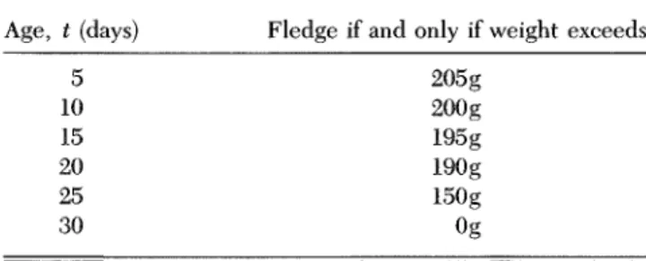
The dynamic programming equations can now be solved to determine the optimal fledging strategy; the results are shown in Table 1. These predictions agree

Table 1. Optimal age and weight of fledging for murres. Age, t (days) Fledge if and only if weight exceeds

5 10 15 20 25 30 205g 200g 195g 190g 150g

Clark: Modeling behavioral adaptations Table 2. Some recently published dynamic programming models.

Reference Mangel 1987 Clark 1987 Houston &

McNamara 1987 Clark & Levy 1988 Ydenberg & Clark

1989

Clark & Ydenberg 1990

Lucas & Walter 1988

Species Parasitic wasps (Nasonia vitripennis) Lions (Panther leo) Birds Sockeye salmon (Oncorhynchus nerka) Western grebes (Aechmorphus occidentalis) Dovekies (Alle alle) Carolina chickadees (Parus carolinensis) Behavior Oviposition Hunting Singing Vertical migration Diving Parent-offspring conflict Food caching Main Prediction Stochastic facultative variation in clutch size Relations between group size and prey type Dawn and dusk chorus Timing of daily migrations Patterns of aerobic and anaerobic diving

Weight recession prior to fledging Environmental influences on caching behavior Empirical (E) or Theoretical (T) E E T E E E E,T

reasonably well with the published data (fledging age from 18-25 days, weight from 150-220 gin). The model also suggests a negative correlation between age and weight at fledging, a prediction that is well supported by the data. Ydenberg concludes that the model is successful and "provides a good general framework for understand-ing the selective forces [affectunderstand-ing] fledgunderstand-ing age and weight . . . " The purpose of discussing this model here, however, has simply been to indicate the practical ap-plicability of dynamic behavioral modeling.

Table 2 lists several additional dynamic-programming models of behavior. The reader may note the wide range of species and behaviors encompassed by this list. In most cases the observed behavior could not have been ana-lyzed successfully without using a dynamic model; in other cases the dynamic model provides insights and predictions that differ from earlier studies. All of these models, however, are what I refer to in section 7 as "first-generation" models.

6. Some misconceptions

The peer commentaries on Houston & McNamara (1988a) expressed a number of misgivings about the dynamic programming approach to behavioral modeling. Table 3 lists eight of these misgivings, each of which I feel is the result of misconceptions. I shall discuss these misconceptions in turn.

Terminal reward function. Houston & McNamara identi-fied the specification of the terminal fitness function $(X(T)) as a major difficulty of the dynamic programming approach. For several reasons I believe the problem to be much less severe than they suggest. First, <&(X(T)) has biological meaning, since it represents expected future reproductive success, i.e., reproductive value (Fisher 1930). (Houston & McNamara's term "reward function" fails to emphasize this important point.) The general form of this function is often intuitively clear - it is usually nondecreasing in the state variable x (within limits - e.g.,

Table 3. Some misconceptions about dynamic programming

models of behavior.

Assertion Commentators*

1. Terminal reward function is hard to specify, but strongly

influences predictions.

2. Dynamic programming models are too general, capable of predicting almost anything, and untestable.

3. Reproduction is not included, so that the models have no direct connection with Darwinian fitness.

4. Evolution does not necessarily lead to optimal behavior; there is experimental evidence of non-optimal behavior (e.g. the matching law).

5. Terminal time may be hard to specify, but strongly influences predictions

6. Dynamic programming models are overly complex; animals use simple decision rules

7. Testing the model's predictions requires measurement of state variables.

8. Solving a dynamic model backwards in time is artificial, and ignores the organism's past.

Barnard, Caraco, Huntingford & Metcalfe, Reid, Sherry, Sih, Stenseth, Timberlake Huntingford & Metcalfe, King & Logue, Partridge, Reid, Timberlake Calder, Huntingford & Metcalfe, Morse, Stenseth Heyman, Fantino Huntingford & Metcalfe, Rachlin, Timberlake Heiner, Yoerg Smith, Yoerg Barnard, Morse

*All references are Behavioral and Brain Sciences 11 (1988), and occurred as peer commentaries to Houston & McNamara (1988a).

Clark: Modeling behavioral adaptations

an overweight bird might experience difficulty flying, or be more subject to capture by a predator), and often involves a threshold value of x, below which survival or reproduction become unlikely. When a precise charac-terization is necessary, the determination of <&(X(T)) by actual measurement of the relationship between state variables and future reproduction is certainly not un-thinkable (see section 7).

Dynamic programming models exhibit an important convergence property, in the sense that the optimal strategy A *(*:,£) converges to a stationary strategy A*(x) that is independent of t, as the "time to go" T — t increases (Mangel & Clark 1988, p. 232; McNamara 1990; McNamara & Houston 1982). Moreover, A*(x) is independent of the terminal fitness function. Conse-quently, if one is interested in modeling behavior not associated with the anticipation of future changes in external conditions beyond the horizon T, then a precise specification of <f>(X(Tj) may not be important. If the modeler is specifically concerned with time constraints, however, as might be the case for studies of migration, diapause, the timing of breeding activities, and so on, then careful estimation of <&(X(T)) may become im-portant.

Ideally, T would be identified with the end of the individual's possible reproductive life span, in which case €>(X(T)) = 0 by definition. The model would then encom-pass the entire life span and be correspondingly more complex than a model of behavior over a limited time period. The method of "sequential coupling" (Mangel & Clark 1988, p. 69) allows one to break up the task of modeling behavior over an entire life span into more manageable submodels over briefer periods. For exam-ple, models of alternating breeding and nonbreeding seasons can be linked together.

To understand sequential coupling, suppose that a model covering the time period from Tx to T2 has been

constructed and solved. Then $Tl(X(T1)), obtained from

this model, represents the individual's expected future reproduction from time Tl on. This function is therefore

the "terminal" fitness function for a model covering a period from To to T1. The two models may have different

environmental parameters, consider different types of behavior, and even use different units of time. In any case, the two models are linked, or sequentially coupled, by virtue of the fact that the initial fitness function <Pr of

the later model equals the terminal fitness function for the earlier model. Any number of such models can be linked sequentially; for example, this procedure is useful for modeling alternating days and nights (McNamara et al. 1987), or alternating seasons.

Backwards indyction. The dynamic programming al-gorithm operates backwards in time from some specified terminal horizon T. This procedure may seem highly artificial. The method becomes less mysterious if one realizes that whenever behavior is considered as a dy-namic phenomenon, the future becomes fully relevant. Every behavioral act has inevitable implications for the individual's future, so that the full implications of behav-ior cannot be understood by looking only at the immedi-ate present. In spite of its uncertainty, the future must always be anticipated; the dynamic programming al-gorithm makes this mathematically explicit. Solving

backwards in time is not artificial; on the contrary it is absolutely unavoidable in any evolutionary theory of behavior.

The assumption of a fixed, known terminal time T may also appear unsatisfactory. But every individual has a maximum possible lifespan, and in a full-life model T can be equated to this maximum lifespan. The possibility that the individual dies before time T is covered by allowing for mortality risks. In a one-season model, T would represent the end of the season. In this case T may be uncertain, rather than a fixed constant. This eventuality is easily dealt with, however: One simply defines T as the last possible date in the season, and includes a probability factor for the actual end of the season at any date t prior to T.

Another possible misconception is that dynamic pro-gramming does not consider the influence of past events on current behavior. But past events affect state variables (which may include memory-related variables). The op-timal behavior a* at time t is a function of the current state variable X(t), and is therefore fully responsive to past events through their effects on the individual's current state.

Reproduction, None of the models described by Houston & McNamara included reproduction explicitly; several commentators concluded that the method could not en-compass reproduction. This is simply not the case, al-though I too have until now ignored reproduction during the modeling interval, for simplicity of presentation. Suppose now that (as shown in Figure 1) behavior in period t leads to immediate reproduction R = R(X(t),A(t),w(t)). Thus reproductive output may in gener-al be affected by the individugener-al's state and behavior, as well as by external stochastic events w(t). By repeating the discussion leading to Equation (9), it can be seen that we now obtain

<S>,(X) = maximum EjR(x,a,w) + &t + 1(G(x,a,w))} (10)

The interpretation of Equation (10) is straightforward: The optimal behavior a in period t is that which max-imizes the sum of current reproduction R(x,a,w) and expected future reproduction Q>t+l(. . .)• The dynamic

programming algorithm, and the logic underlying it, go through unchanged.

Additional complications may arise if current behavior affects future reproduction, but this possibility can be encompassed by introducing additional state variables. An example would involve the acquisition of territory or mates prior to breeding, in which case state variables representing territory size or number of mates would be included in the model.

The state-variable dynamic modeling framework is extremely flexible. Indeed, this very flexibility can itself be problematic; it is easy to design a complex dynamic model that goes far beyond available data. Also, computa-tional difficulties in dynamic programming expand expo-nentially with the dimension of the model. These ques-tions are discussed further in secques-tions 7 and 10. Testability. The idea that dynamic programming models are untestable is incorrect. When constructed using em-pirical data, they provide quantitative predictions that

Clark: Modeling behavioral adaptations can be tested directly against field or laboratory data.

Theoretical, data-free models can be developed to gener-ate qualitative predictions, and these can also be tested against known behavior. Empirical testability is one of the most important features of the dynamic modeling framework described here.

Dynamic behavioral models are more readily testable than it may appear. Suppose that the optimal behavioral strategy a*(x,t) has been obtained for a certain model by solving the dynamic programming equations. Substitut-ing this optimal behavior into the equation of system dynamics

X(t = G(X(t),a*(X(t),t)9w(t))

results in a time-dependent Markov chain (or a time independent chain if a* is stationary). By iterating this chain forward in time one can generate probability dis-tributions of the state variable X(t) over time. From this state distribution, one then immediately deduces the distribution of behavior over a population of similar organisms. The latter distribution is testable against be-havioral data without requiring detailed knowledge of the actual states of organisms in the population. Mangel (1987) gives a very simple example concerning oviposi-tion in parasitic insects, showing that wide variaoviposi-tion in clutch sizes should be expected. This prediction agrees well with the data (Charnov & Skinner 1.984).

Excessiwe generality. Dynamic programming models are flexible, but to dismiss the method as too powerful -"capable of proving anything" - would be to misunder-stand of the role of theory in science, tantamount to refusing to use the electron microscope because it reveals too much detail. Mathematical, statistical, and experi-mental techniques can be, and often are used incorrectly, but banning them is hardly the remedy. The predictions derived from any model depend on the assumptions used in its formulation. If the predictions disagree with obser-vation, the model must be rejected, and new models must be sought. The model may be completely wrong-headed, or perhaps only some of its components are inaccurate, needing to be modified or replaced. Each component should be examined for biological veri-similitude; indeed separate testing of component hypoth-eses may often be feasible. This sequence of model formulation, testing, modification or replacement, and testing again, is the cornerstone of scientific research. Qptimaiity hypothesise Whereas it is certainly true that evolution does not always maximize fitness, proponents of the claim that fitness is seldom or never maximized place themselves in the position of having to find some novel explanation for the almost universal occurrence of behavioral adaptations in nature. I prefer to accept adap-tation as a hypothesis and would be surprised by any incontrovertible evidence to the contrary.

Several of Houston & McNamara's commentators cite the matching law of operant psychology as evidence of nonoptimal behavior, without explaining why it contra-dicts optimality. It may seem obvious that an optimizing subject should stick to a superior alternative, once it has learned which this is, but how is the subject to know that one alternative is destined (by experimental protocol) to remain forever superior? If temporal variability of the

environment is the rule in nature, adaptive behavior would require the use of sampling strategies capable of tracking a changing environment (Stephens 1987). Sam-pling behavior described by the matching law has this characteristic.

Simple decision rules. Another worry of Houston & McNamara's commentators was that animals may not be able to solve dynamic optimization problems the way computers do. They may be limited to using simple decision rules. This argument is flawed in several re-spects:

First, decision rules are exactly what a dynamic pro-gramming model produces. No one imagines that animals actually compute these decision rules by dynamic pro-gramming - fitness maximizing behavior is selected by the evolutionary process. The strategy derived from a dynamic optimization model may conceivably be too complex for organisms to use, but unless we have some idea of the optimum optimorum we cannot assess the degree of adaptation that observed behavior represents. The feeding of parasitic nestlings might be quoted as an obvious example of maladaptive behavior, but if the nesting season is well advanced by the time that the pseudoparent would be able to detect the fraud, the selection pressure for learning to recognize and abandon parasitic nestlings may be quite small. Similar arguments apply in general to the interpretation of predictions derived from optimization models (Houston & Mc-Namara 1986). Unless the predicted behavior is signifi-cantly superior to alternatives, selection pressure favor-ing its evolution may be weak. Even though quantitative testing of an optimization model may be feasible, the qualitative predictions are often more interesting and informative than the exact quantitative predictions (Fa-gerstrom 1987).

The claim that animals use only "simple" decision rules begs the question of characterizing simplicity. If it can be shown that a certain simple rule performs almost as well as the more complex rule obtained from an optimization model then there is clearly no reason to expect the complex behavior to evolve. The relative effectiveness of the two rules can only be assessed on the basis of some model, however; dynamic models are particularly well suited for this comparison. At any rate, I am unable to imagine how a theory of behavior with an evolutionary basis could be constructed by restricting consideration to some predetermined class of "simple" decision rules. It is not the simplicity of behavior that usually astounds us but its complexity.

7. Data requirements and model deweiopment Every model is a deliberate simplification of the real world. Where, then, does one draw the line in terms of complexity in designing a given model? Simple models help us organize our understanding of nature, but invari-ably lack realistic detail.

The data available are an important consideration in model development. Models that vastly outstrip the available data may be popular with theoreticians, but they contribute little to science.

Clark: Modeling behavioral adaptations

some parameters for which the necessary data are in-complete, however. One of the main purposes of model-ing is the quantitative testmodel-ing of novel hypotheses, which often means that the appropriate data have never been collected since their relevance was unsuspected. With reasonable guesses for unknown parameters one can complete the model and see whether it gives interesting and reasonable predictions. If so, the necessary data should be sought.

Many models are probably best abandoned at this early stage. If the model shows promise, however, it may be tentatively accepted as a "first-generation" model. The requisite experiments to estimate parameters and test its predictions may be designed and performed. During this process new information may come to light, and a second-generation model may be developed.

The methodology for dynamic behavioral modeling in biology is sufficiently novel that few if any such first- and second-generation sequences have yet been published. This kind of research is actively being pursued in several laboratories; I predict that such activities will expand in the future.

8. Enwironmental uncertaintf

The dynamic modeling techniques discussed above can be extended to deal with a variety of additional phe-nomena, the main limitations being the availability of data and computational complexity (see sect. 10). For example, an external environmental state variable Y(t), as in Figure 1, can be included. This is relatively straightfor-ward, provided one assumes that the individual always has complete information about the environment before making any behavioral decisions. A much more interest-ing and difficult situation arises when the individual's knowledge of its environment is imperfect, which will often be the case in fluctuating environments.

Under these circumstances, the individual's state vari-able X(t) can be expanded to include the current infor-mational state about the environment. The current be-havioral decision then depends on the individual's physiological and informational state variables but not on the current environmental state directly. Here we enter into the subject of dynamic decision theory under bona fide uncertainty, involving imperfect information about the present as well as the future state of the environ-ment. Behavioral decisions must now include the pos-sibility of deliberately sampling the environment so as to reduce this uncertainty, facilitating more effective future decisions. In spite of its obvious importance in behav-ioral biology, hardly any work has been done in this area (recent references include Stephens 1987; Mangel & Clark 1988, Chapter 9; and Mangel 1990). It seems to me that the biology of learning will not be well under-stood until this theory has been much more fully developed.

game theory

Figure 1 overlooks an extremely important aspect of the evolution of behavior, namely that the behavior of any one individual inevitably affects and is affected by the

behavior of many other individuals. Thus the behavioral landscape really consists of a large collection of individual landscapes, with numerous interconnections represent-ing predator-prey, competition, kinship, and other rela-tionships.

Behavioral interactions have been extensively model-ed using game theory, particularly the concept of an evolutionarily stable strategy (ESS) (Maynard Smith 1982); [See also Maynard Smith: "Game Theory and the Evolution of Behavior" BBS 7(1) 1984.] An ESS is a behavior strategy that makes the best of the circum-stances, in the sense that, if adopted by the members of a population, it is not subject to invasion by a rare mutant alternative strategy. ESS models are usually somewhat difficult to analyze and tend to become much more difficult when made explicitly dynamic. The few pub-lished dynamic game-theoretic models of animal behav-ior have been based on strong simplifying assumptions (Clark & Ydenberg 1990; Houston & McNamara 1987; 1988b).

For example, in a model of fledging behavior taking account of parent-offspring conflict (the offspring wishes to be pampered), Clark & Ydenberg (1990) assumed that the decisions made by the parent and its offspring alter-nate sequentially. This facilitated a fairly straightforward dynamic programming computation of the ESS. The model was applied to fledging data for dovekies (Alle alle), a small Arctic-breeding seabird, and provided a behav-ioral explanation for the phenomenon of prefledging weight recession in this species. This is one of a very small number of game-theoretic models attempting quan-titative predictions and may indicate a potential for the development of data-dependent ESS models.

10. Limitations

Critics and defenders of optimization modeling in biology abound (e.g., Gould & Lewontin 1979; Grafen 1984; Maynard Smith 1978; Mayr 1982; Oster & Wilson 1978; Pierce & Ollason 1987; Stephen & Krebs 1986). One can agree with the critics that the adaptationist paradigm has often been carried to extremes, and that evolution is at best an imperfect optimizer, while at the same time accepting the fact that optimization models - and their relatives, game-theoretic models - can be extremely useful in organizing our understanding of observed phe-nomena. Many recognized limitations of traditional op-timization models of behavior succumb completely to the dynamic modeling framework described in this target article.

Indeed, the flexibility of dynamic state-variable models may itself become a source of trouble. The temptation to construct exceedingly complex dynamic behavioral mod-els, naively thought to capture the "real complexities" of nature, could lead to a plethora of incomprehensible models, as has already happened in areas like systems ecology. It is always hard to prevent people from mis-using powerful scientific techniques that they don't un-derstand (think of statistics!).

The ©yrse of dimensionality. Dynamic optimization theo-ry has its roots in the calculus of variations, developed in the 18th and 19th centuries by Euler, Lagrange,

Clark: Modeling behavioral adaptations Weierstrass, and other mathematicians. The

require-ments of modern technology, particularly communica-tions and space exploration, led to the reformulation and extension of the classical calculus of variations in terms of optimal control theory (Pontrjagin et al. 1962) and dy-namic programming (Bellman 1957). These methods, which are now routinely applied in many fields, including engineering, operations research, and economics, have been further enhanced by the spectacular increases in computing power that have occurred simultaneously. It was inevitable that these developments would eventually affect behavioral biology.

In principle, dynamic programming and optimal con-trol theory are capable of encompassing arbitrarily com-plex dynamic decision problems. Practical limitations are reached quite rapidly, however, as the dimensionality of the state space increases. This so-called "curse of dimen-sionality" (Bellman's term) is not a feature of any particu-lar modeling approach or algorithm but is an intrinsic characteristic of dynamic optimization problems with many state variables.

The difficulties are twofold. First, model identification (choice of functional forms, estimation of parameters, etc.) obviously becomes more difficult as the scope and complexity of a model increases. There may be tradeoffs between a model's degree of realism and the ability to identify the model from available data (Ludwig 1989). Second, computational requirements in terms of mem-ory and numerical calculations increase as nm, where m is the number of state variables and n the number of discretized values used to represent each state variable. For m larger than 4 or 5 these requirements begin to exceed the capacity of large computers. These limitations are particularly relevant for models including environ-mental uncertainty, since now the informational state must also be included, significantly increasing the dimen-sionality and complexity of the model. Similar problems arise in ESS models of pairwise contests, since the state variables of both contestants must be included.

The curse of dimensionality necessarily arises in any attempt to solve dynamic optimization, or dynamic game models. These problems are inherently complex (unless they are of low dimension); no revolution in optimization theory is likely to overcome this fact. An intriguing possibility is to use the computer to emulate the evolu-tionary process in searching for optimal or ESS strategies via a process of natural selection, but to my knowledge this has not yet been attempted.

The characterization of fitness. In this target article I have assumed that an organism's fitness is adequately described by its total expected lifetime reproductive output. It is well known that this definition is not always appropriate, particularly for growing or age-structured populations, or for populations in stochastic environ-ments (Cohen 1966; Levins 1968; Stearns 1976). One adjustment, replacing the arithmetic mean with the geo-metric mean, is easily accomplished (Mangel & Clark 1988, p. 240), but combining behavioral and population genetic models in general would appear a daunting pro-ject (see Yoshimura & Clark in press). Grafen's (1984) discussion of the "phenotypic gambit" in behavioral mod-eling is relevant to dynamic as well as traditional static optimization models.

The functional analysis of behavior is by definition based on the Darwinian paradigm of natural selection according to survival and reproduction. Since these processes trans-pire over time, it follows that the time dimension must somehow be taken into account in any such analysis. Simplifications may sometimes be adopted so as to finesse the time dimension, but timeless models have narrow limitations which preclude the analysis of many impor-tant aspects of behavior.

Dynamic optimization techniques are significantly more difficult than static methods. Recent experience with dynamic programming models of behavior, how-ever, has indicated many advantages for this approach. The restrictive assumptions (linearity, convexity, deter-minism) underlying such alternative techniques of dy-namic optimization as optimal control theory become irrelevant when optimal strategies can be deduced via numerical computation. Dynamic programming models are extremely flexible and can be used to study an almost unlimited variety of behavioral phenomena. State vari-ables and model parameters have operational signifi-cance, so that empirical testing of a model's predictions is feasible.

More important, the dynamic approach to behavioral modeling provides a completely different outlook on behavioral theory, compared, say, to the traditional mod-els of foraging theory (see Fantino & Abarca 1985), or to models based on economic concepts like utility or indif-ference contours (see Rachlin et al. 1981). The entire manifold of tradeoffs ("costs and benefits") typically asso-ciated with any behavioral decision can be conceptualized and modeled in a consistent and unified way. Dynamic programming models are a natural extension of the ac-cepted approach to the modeling of life-history traits (Horn & Rubenstein 1984).

It is only to be expected that a modeling framework so capable of encompassing realistic complexities will have practical limitations. The art of modeling consists in finding a happy compromise between simplicity and complexity which will enhance our understanding of nature.

When should dynamic as opposed to static or averaging models be considered in behavioral theory? Quantitative models are by nature less general than qualitative ones; this should be taken into account in choosing the model-ing framework. My experience in behavioral modelmodel-ing suggests that the possibility of designing a dynamic model should be thought about whenever quantitative predic-tions and testability are desired, or whenever the trade-offs between different behavioral options are of interest. None of the standard simple models of behavioral ecology have stood up particularly well to quantitative tests (Ste-phens & Krebs 1986, Chapter 9), although their success in providing qualitative insights should not be under-rated.

ACKNOWLEDGMENTS

Alasdair Houston, Marc Mangel, John McNamara, and Ronald Ydenberg sent me their detailed comments on the first draft, leading to a thorough revision; I thank them heartily. The final draft took advantage of the suggestions of several BBS anony-mous referees. My research is supported in part by an NSERC (Canada) grant 83990.

Commentary/Clark: Modeling behavioral adaptations

Commentary submitted by the qualified professional readership of this journal will be considered for publication in a later issue as Continuing Commentary on this article. Integrative overviews and syntheses are especially encouraged.

tmic models of behavior: Promising

Isky

Thomas R. Alley

Department of Psychology, Ciemson University, Clemson, SC 29634-1511

Eteetronie mail: alley@clemson.bitnet

In his target article, Clark presents both the strengths and the weaknesses of a promising dynamic state-variable model of behavioral adaptations. Although he is careful to point out that such models are inherently limited by the complexity of ecologi-cal systems, we are left wondering just how useful dynamic optimalization models can be. Moreover, such models pose a greater risk of misguiding theory and research than Clark's paper suggests.

Mathematical models of complex phenomena typically pro-duce predictions and conclusions that err, to some degree, in a quantitative fashion. Quantitative errors are certainly to be expected for dynamic models of behavior, particularly because the functional contribution of any behavior can be evaluated only within an immensely complicated ecological context. Hav-ing forewarned us of the difficulties of producHav-ing models that make satisfactory quantitative predictions, Clark ends his article with the admonition not to underrate the ability of models in behavioral ecology to provide qualitative insights. I encourage behavioral ecologists not to overrate the ability of dynamic models to provide qualitative insights. Faulty assumptions, poor parameter estimation, and over-simplification can all prove fatal. Some earlier mathematical models in ecology show that (simplified) models of ecological processes can lead to serious qualitative errors. As a prominent biologist said, mathemati-cians need to avoid "developing biological nonsense with math-ematical certainty" (Slobodkin 1975).

The mathematical treatments of competition provide a good example of such pitfalls in mathematical models. One potential pitfall consists of starting from false assumptions. Until recently, "virtually all mathematical treatments of competition" assumed competitive equilibrium (Wiens 1977), yet true competitive equilibrium occurs rarely, if at all, in nature (Alley 1982; Pianka 1976). The simplifications required to construct tractable mod-els introduce additional perils. Classical competition modmod-els adopted such simplifications as stability in environmental condi-tions and limited genetic variation. The resultant models pre-dicted the eventual extinction of one of two competing but coexisting populations, thereby supporting the influential prin-ciple of competitive exclusion. Moreover, lab experiments with simple homogeneous environments have demonstrated com-petitive exclusion (Hardin 1960). Modest changes in the mod-els, however, indicate that coexistence of competitors may be possible (Vandermeer 1975), as field biologists believe (e.g., den Boer 1980). In retrospect, it is clear that neither the artificially simple laboratory studies nor the corresponding com-petition models actually generalize to natural communities (nor should they be expected to).

The newer, more sophisticated dynamic models advocated by Clark (target article) and Houston and'McNamara (1988) are much less likely to make fatal assumptions about stability in environmental, genetic, or behavioral conditions because the interrelated changes in these state variables are directly incor-porated in the models. Furthermore, it appears (cf. Clark's

Equation 1) that dynamic models will follow the rule that adaptedness must always be assessed in the context of an explicit environment (Slobodkin & Rapoport 1974). Dynamic models also allow the environment to be defined in terms of the functional characteristics of organisms, as must be done to capture the fundamental ecological characteristic of mutual compatibility between organisms and their natural environ-ments (Alley 1985). Nonetheless, serious qualitative errors may arise from the processes of simplification, variable selection, and parameter estimation required by dynamic modeling.

Viable models of behavior require careful attention to ecologi-cal details (Houston & McNamara 1988) and even then may fail completely. The act of consuming a resource can be used to illustrate this difficulty.

It is reasonable, and often correct, to assume that consuming a nutritious food resource will usually make a positive contribu-tion to an organism's fitness. Hence a modeler of behavior may estimate some positive value of this behavioral act, and laborato-ry experiments may support the model. Nonetheless, the resul-tant model may provide a highly distorted picture of the contri-bution to fitness made by a tendency to seek and consume this resource. For instance, if consuming this resource will result in potentially lethal exposure to a predator or harmful interactions with a superior competitor, the act of consuming this item may have a negative value. Energy costs, resource scarcity, water reserves, and many other factors influence the value of this behavior (Houston & McNamara 1988). In short, the value of this act, like almost any other behavior, may easily be mis-judged.

In conclusion, dynamic behavioral models have (potentially) sufficient breadth of applicability and power to be useful in behavioral ecology. Their development forces modelers to spec-ify precisely the most important state variables and the dynamic changes in state across time; this may prove to be a helpful guide to research. These models may provide a good way to test our understanding of behavioral ecology, but they are not to be trusted without substantial empirical support from field investi-gations. They may provide insight into optimal behavioral strat-egies, the nature of differences between taxonomic units, and ecological relationships, but are likely to yield only an approx-imation of true optimal behavior. I wholeheartedly agree with Clark that the modeling needs to be treated "as a process of successive approximation to . . . nature," with the models themselves continually tested against data from laboratory and field studies.

Learning and incremental dynamic

programming

Andrew G. Barto

Department of Computer and information Science, University of Massachusetts, Amherst, MA 01003

Electronic mail: barto@cs.umass.edu

It would be surprising if a computer scientist interested in the adaptive behavior of both natural and synthetic systems were to find significant grounds for criticizing the approach to behavior modeling described in Clark's target article. Optimization theo-ry has unquestioned utility in the design of synthetic adaptive systems (with fruitful debate centering on what to optimize and how best to do it), and the concept of a dynamic system's state has proven to be one of the most powerful in modern engineer-ing. Indeed, it is surprising to me that the theoretical framework described by Clark has not been more widely adopted by behavioral scientists. The complexity of animal behavior de-mands the application of powerful theoretical frameworks. The point of my commentary is to suggest that beyond its role in evolutionary biology, the dynamic modeling technique

de-Commentary/Clark: Modeling behavioral adaptations

scribed by Clark can also provide an approach to modeling animal learning at the mechanistic level.

Clark indicates that the dynamic modeling techniques he discusses are highly relevant to the biology of learning. If an animal's internal state includes information about the animal's current knowledge of its environment, then dynamic program-ming methods can be used to generate decision rules that take into account the utility of gathering information in the same way that they take into account the utility of gathering food. I agree that this is an important area of research that has not yet been developed (although the statistics literature contains relevant work; see, for example, Berry & Fristedt 1985). Dynamic modeling techniques and dynamic programming, however, can contribute to our understanding of learning in ways not sug-gested in the target article.

Clark says "no one imagines that animals actually com-pute . . \ decision rules by dynamic programming - fitness maximizing behavior is selected by the evolutionary process." But some of us do imagine that animals actually use methods that incorporate principles of dynamic programming to adjust behavioral strategies while they are behaving. I wish to bring to readers' attention a growing body of research in which learning tasks are modeled as dynamic optimization problems and the learning system itself is engaged in a kind of dynamic program-ming. Instead of computing behavioral strategies that maximize evolutionary fitness, however, the learning system uses dynam-ic programming principles to adjust behavioral strategies to improve the total amount of "payoff" that can be accumulated over time. Payoff can be thought of as a measure reflecting the learning system's preference ordering over combinations of environmental states, internal states, and behavioral acts, to use Clark's terminology. The means by which circumstances gener-ate levels of payoff are "hard-wired" by an evolutionary process, but a behaving system can adjust the details of its behavioral strategy to improve payoff yield over time.

From an engineering perspective, the learning problems treated according to this view are adaptive optimal control problems in which the complexity of the system to be controlled and a lack of complete prior knowledge about its dynamics prevent the prespecification of an optimal, or even useful, control rule. Unlike most mathematical formulations of learning tasks (such as those widely adopted in the field of artificial neural networks), this formulation encompasses tasks in which the consequences of an action can emerge at a multitude of times after the action is taken, and both short-term and long-term consequences must be considered in generating control actions. On the surface, however, because it proceeds backward in time, dynamic programming would appear to be a very poor candidate for modeling learning mechanisms that operate in real time. How can dynamic programming be accomplished by a learning system unless it uses large data structures and exten-sive off-line processing, that is, unless it is "able to solve dynamic optimization problems the way computers do"? In addition, dynamic programming seems irrelevant as a learning procedure because it requires a detailed knowledge of the system's dynamics, knowledge not directly available to the learning system.

These properties do rule out a literal form of dynamic pro-gramming as a model of real-time learning, but there are simple rules for updating memory structures during behavior that can approximate incrementally what would be computed by a literal form of dynamic programming. In addition, such rules can do this without complete knowledge of the underlying dynamic system. These rules are based on the same recursive tionships exploited by dynamic programming, but these rela-tionships are applied during behavior. If a learning system can experience varied and repetitive interaction with a dynamic environment, it can incrementally approximate the results of dynamic programming while always going forward in time. Moreover, the learning rules allowing this are not much more

complicated than other incremental learning rules that have been put forward as models of animal learning, for example, the Rescorla-Wagner model of classical conditioning (Rescorla & Wagner 1972), or rules used in synthetic systems, such as the Widrow-Hoff rule (Widrow & Hoff 1960).

The study of on-line learning methods for approximating the results of dynamic programming has been directed both toward designing synthetic systems and toward modeling animal learn-ing. The use of these methods has been called "heuristic ic programming" (Werbos 1977; 1987) and "incremental dynam-ic programming" (Watkins 1989). The "temporal difference" (TD) methods analyzed by Sutton (Sutton 1984; 1988) and used in some adaptive control experiments by Barto et al. (1983) are examples of this class of method. Models of animal learning which use principles of dynamic programming include the TD model of classical conditioning of Sutton & Barto (1987) and the model of Klopf (1988) and Klopf & Morgan (in press). The TD model provides an account of a range of classical condition-ing phenomena with a simple learncondition-ing rule based on incremen-tal dynamic programming. Further discussion of these ideas, their history and relation to dynamic programming, as well as references to other relevant research, are provided by Sutton & Barto (in press) and Barto et al. (in press).

As this approach to animal learning develops, its appeal to optimization theory is likely to become even more controversial than is the appeal to optimization theory in behavioral ecology. If anything, justifying a specific definition of "payoff" for a learning task is more problematic than defining evolutionary fitness, and the canonical example of nonoptimal behavior -matching behavior in operant conditioning - more directly concerns learning than evolution. I would suggest, however, that, to paraphrase Pope, a little optimization theory is a dan-gerous thing. In engineering design, performance criteria must either reflect what the designer really wants, or their optimiza-tion can yield totally unsatisfactory results (a point emphasized by Norbert Wiener (1964) by reference to Goethe's poem The

sorcerers apprentice). In a theory of behavior, explanations in

terms of optimization criteria that do not reflect the true com-plexity of a task are inadequate and misleading. Significant progress in understanding learning can be made by adopting optimization criteria that take into account internal and external states, system dynamics, and the temporally extended nature of behavior.

ACKNOWLEDGMENTS

I wish to thank John Moore and Dorothy Mammen for helpful evalua-tion of drafts of this commentary.

Gaps in the optimization approach to

behavior

Patrick Colgan and Ian Jamieson

Department of Biology, Queen's University, Kingston, Ontario, Canada, K7L 3N6

Electronic mail: colganp@qucdn.bitnet

Although the target article is a clear and succinct exposition of dynamic modeling, the applicability of this approach is not as general as Clark maintains. The purported comprehensiveness of such modeling is symptomatic of the narrowness which would make ethology a one-legged monster (Dawkins 1989). These failings can be seen by focusing on the methodological basis of the approach, the rule of phylogenetic and developmental constraints, and the issue of mechanisms.

Contrary to Clark's assertions (sect. 1), the optimization approach may serve more to canalize, rather than organize, our explanations of animal behavior. Clark adopts the hypothesis of optimal adaptation as axiomatic based on many undisputed supporting examples. This stance is quite different from that