Robust Methods for Credibility

BY HANS R. KUNSCH

ETH, Zurich, Switzerland

ABSTRACT

Excess claims lead to an unsatisfactory behavior of standard linear credibility estimators. We suggest in this paper to use robust methods in order to obtain better estimators. Our first proposal is the linear credibility estimator with the claims replaced by a robust M-estimator of scale calculed from the claims. This corresponds to a truncation of the claims with a truncation point depending on the data and different for each contract. We discuss the properties of the robust M-estimator and present several examples. In order to improve the perfor-mance for a very small number of years, we propose a second estimator, which incorporates information from other claims into the M-estimator.

KEYWORDS

Robust statistics; credibility; big claims; M-estimators; influence function. 1. INTRODUCTION

This paper attempts to introduce robust methods into the area of credibility. In many actuarial applications excess claims (outliers) which are much bigger than ordinary claims do occur. Excess claims inflate the variance of the claims within a contract and thus lead to a small credibility factor. This means that linear credibility charges almost the same premium to contracts which did not incur an excess claim even when their individual experience is quite different otherwise. On the other hand, despite the small credibility factor, those contracts which incurred by bad luck an excess claim have to pay a high premium. This unsatisfactory behavior of linear credibility is illustrated in Example 5.3 below. It is taken from GISLER (1980a, b) where he proposed the following solution to this problem: He truncates all claims above a certain level which is determined from the whole portfolio so as to minimize mean square error. It seems however that this method is difficult to use in more complex situations, e.g. for hierarchical credibility or when only claim rates with different volume measures are available. As a theoretician I also wondered if a single truncation level for all contracts is always appropriate. For further discussion of excess claims in credibility we refer the reader also to the paper by GISLER and REINHARD (1990).

Robust statistics has had an enormous development during the past 25 years. According to HAMPEL et al. (1986) "In a broad informal sense, robust statistics

34 HANS R. KUNSCH

is a body of knowledge, partly formalized into 'theories of robustness', relating to deviations from idealized assumptions in statistics". In particular this body of knowledge contains some clever estimation methods which are much less affected by outliers than their classical counterparts. They were developed when studying heavy tailed deviations from distributional assumptions. These robust estimators are thus good candidates for dealing with the excess claims in credibility. In several respects the situation in credibility theory is, however, different from the one usually considered in robustness: For instance in credibility nonparametric methods prevail whereas robustness studies a neigh-borhood of a specific parametric model; credibility is interested in all the data, not only in the majority, because premiums have to cover all claims; the parameters one is estimating in credibility theory are random and not fixed like in the framework of robust statistics. Maybe for these reasons the two fields have been largely separated until now. Because of these differences we were not able to derive our estimators from a general principle or an optimality criterion. We just propose some simple estimators which are based on heuristic considerations and seem to work reasonably well. In our first proposal we calculate a robust estimator from the claims of each contract and use then linear credibility based on these estimators instead of the original claims. In the second proposal we incorporate an a priori premium into a robust estimator based on the claim sizes in a nonlinear way. Here we are inspired by some Bayesian estimator. The resulting estimator is, however, free from any distri-butional assumptions.

With these proposals I hope to convince actuaries that robustness can make a contribution to the problem of excess claims and that further research is worthwhile. In particular I am convinced that the methods proposed here can be adapted to hierarchical credibility and models with different volumes. Some preliminary work is in GISLER and REINHARD (1990), but this is a topic for a future paper.

2. MODELS AND ESTIMATORS

We consider the basic credibility model with J contracts and n years of experience. It contains unobservable risk parameters 0j and claims sizes Xtj > 0

(1 < / < n, 1 <j < J). We make the following distributional assumptions: (2.1) (6j ,Xlj,..., Xnj) are i.i.d. (1 < j < J),

(2.2) 6j is distributed according to U(dO),

(2.3) Given 8j, X{j, ..., Xnj are i.i.d. with distribution Fg(dx).

It will be convenient to distinguish between the following two situations: Case I : U and Fg are known. In this case a single contract is sufficient, and

we drop the index j . Case II: U and Fe are unknown.

Our goal is to estimate fij = //(#,) = Eg.[Xjj], the pure risk premium. In

Case I we propose

(2.4) 1Z())~= n + *(T(X

...,X

)-E[T})

where n = E[fi(6)] = J//(#) U(dd) is the overall mean and a is the credibility factor. With a chosen to minimize the mean square error, this is the linear credibility estimator based on T instead of Xx, ..., Xn. As our pure experience

based estimator T we take a robust estimator defined implicity as the solution of

n

(2-5) X XiXflT) = 0

with %(z) = max ( - c , , min ( z - 1, c2)) and 0 < c, < 1, 0 < c2. In Case II we

replace means by averages:

(2.6) ft=X.. + a(Tj-T.)

where X = (nJ)~l E, S, Xo, T = J'"' Iy 7} and 7} is defined as the solution

of

(2.7)

with x as above.

We list here some simple properties of our proposal which serve as a first justification:

a) It is scale equivariant: If all Xt {Xy) are multiplied by a constant c, then

/x(oj(fi]) is multiplied by the same constant.

b) It includes the linear credibility estimator: If c, = 1, c2 = oo, then

T = X_ = n~l I , Xi and 7} = Xj = «"' 2,Xy.

c) It is unbiased: E[fi(d)} = fi and J [ 'L'pJ = Xm%. In order to achieve this, we had to use the nonrobust mean Z . in (2.6). From a pure robustness point of view, it would be preferable to take / ^ = (1 — a) 71. + <x7}. However for insurance, unbiasedness is indispensable. Note that we arrive at ^ b y adding the excess X_—J~x 2y/ ^ = X - T to all contracts.

d) It is related to the truncation estimator by GISLER (1980a, b): (2.5) can be written as

(2.8) T = «"' X m a x (0 - c i ) T, min (X,, (1 + c

; = i

i.e. claims on both ends are truncated if c, < 1. The main difference to GISLER (1980a, b) is that the truncation point depends on the contracts experience and is given implicitly.

The estimator (2.5) belongs to the class of so-called M-estimators of scale. These are standard estimators in robust statistics, see HAMPEL et al. (1986,

36 HANS R. KUNSCH

Chap. 2). Their most important property is that the change due to an additional observation at x is approximately proportional to x(x/T). Hence by truncating claims on both ends we bound the influence not only from large claims but also from small ones. In most applications truncation from above alone will be sufficient. However as will be shown in Section 3.2, the estimator may become zero easily if c2 is very small and C\ = 1. From the discussion there the role of the constants cx,c2 will become clearer. It will be seen that their choice is not very crucial and can be done beforehand without having much information about the claims. The credibility factor a on the other hand must depend on the distributions U and Fo in Case I and on all the data in Case II. How this can be done is the content of Section 4.

We use a scale estimator instead of the more common location estimator because we think that in insurance applications it is more realistic to choose

Fe(dx) as a scale than a location family. This takes into account that claims are necessarily nonnegative and that larger mean values entail also larger vari-ances. The scale equivariance (a) above is a direct consequence of using a scale estimator.

3 . DISCUSSION OF THE ROBUST ESTIMATOR We consider only a single contract.

3.1. Existence, uniqueness and calculation of the estimator

Denote by x(1) < x(2) < ... < x(n) the ordered sample and by k0 the number of zero values in the sample. Furthermore we introduce the set of solutions for the equation defining T:

L = L{xx,...,xn) =

Existence and uniqueness of T is covered in the following:

Lemma 3.1: If k0 < nc2/(cl + c2), then L is a closed, finite, non-empty interval.

lfk0 = nc2l{cx+c2) then L = (0, x(to+1)/(l +c2)]. If k0 > /ic2/(c, + c2), then L is empty.

Proof: For any x > 0, t -* x(x/t) is continuous and monotone decreasing.

For t > *(„), Z/iXj/t) < 0. For t < x(k(t+l)/(\ +c2) we have

The case where L contains more than one point does occur, e.g. n = 4, c, = c2 = 0.5, x, = x2 = 0.4, x3 = x4 = 1.8 gives L = [0.8, 1.2]. If a unique

definition of T is needed, we will take the midpoint of L. In case where L is empty, we take T = 0.

The defining equation for T can also be written in the following equivalent form with x(0) = 0, x(n+1) = oo, compare (2.8):

(3.1) T =

(3.2) (3.3)

For given /, and l2, T can be computed from (3.1) and then (3.2) and (3.3)

can be checked. Because l{, l2 can take only a finite number of values, T can be found by trial and error, at least for n not too big. In a more systematic iterative procedure one determines new values lx and l2 such that (3.2) and (3.3) are satisfied and then computes a new Tfrom (3.1) etc. In our experience this worked very well, but we didn't try to prove the convergence of the algorithm. Note that if it converges, it does so in a finite number of steps. An alternative algorithm can be obtained by rewriting (2.5) as

n

«~' Z

x(x,m = i

1=1

with x(z) = max (1 —cx, min (z, 1 + c2)). This suggests the iterative algorithm

I

= i - i x(

Xi/T(m))\ T(m).

1/2

Its convergence follows from HUBER (1981) Section 8.6.

3.2. The breakdown point

In Lemma 3.1 we have already seen that with less than nc2/(cl + c2) zero claims the estimator stays away from zero. Here we consider the opposite case: What is the maximal number of claims tending to infinity for which the estimator remains bounded? In robustness this is called the finite sample breakdown point, c.f. HAMPEL et al. (1986, Sec. 2.2a). The breakdown point plus one is then the minimal number of outlying claims needed to take the estimator to infinity.

Lemma 3.2: Let k = min {i e IN; / > n c{ /(ct + c2)}. Then T remains bounded if

less than k observations tend to infinity, but it tends to infinity if k or more observations tend to infinity.

38 HANS R. KUNSCH

Proof: By definition of k

(3.4) k{ and

(3.5) ( * - l

First we assume that jc(B_i+1) is fixed and derive an upper bound for T: If

ci < 1 we put t = x(n_fc+i)/(l-Ci). Then by (3.5)

1=1 Hence by monotonicity T < t. If C] = 1, we put n-k+l By (3.4) we obtain (1 + c2)t > x( n_t + 1), hence n n-k+l

x(xi/t) ^ /-i x(i)lt~(n — k+ \) + (k — \)c2 = 0.

Moreover for t'> t we have x(x(n-k+i)/t')< X(x(n-k+])lt)- Therefore

2,jX(Xj/t') < 0. This implies T < t and thus completes the proof of the first

part.

For the second part we put t = Jc(n__A:+1)A;/(«c1 + k(l — c,)). By (3.4)

(l + c2)t>x{n-k+l). Hence

Hence the right endpoint of L = {t'; Z,/(x,//') = 0} is > /, and / -» oo if Lemmas 3.1 and 3.2 show that the tolerance towards zero values and outliers are in conflict. This is not difficult to show in general for scale equivariant continuous estimators. A reasonable compromise might be to take c, = c2, but

if a priori knowledge about the claims is available other choices are possible.

3.3. Linearization of the estimator

For the credibility factor a in (2.4) and (2.5) we need the variance of Tand 7}. Because of the implicit definition, this seems hopeless. There is, however, a

simple asymptotic approximation. With the help of the so-called influence function we can linearize T (see HAMPEL et al., 1986, Chap. 2):

(3.6) T(Xl,...,Xn)= T(6) + n-[YJ IF {Xl,

/ = i Here T(d) is defined implicitly by

(3.7) f x(x/T(0)) F

(dx) = 0

and the influence function IF is given by

(3.8) IF(x, 6) = X(x/T(d)) T{6f

where

» (.(l + c2) T(0)

(3.9) M(0)= \ X'(x/T(d))xF0(dx)= \ xFg(dx).

J J(l-e,)r(0)

In particular we have £9[/F(,r,, 0)] = 0, hence Ee[T(Xu ..., Xn)] x T(8),

and

(3.10) Var,[T(X{, . . . , Xn)} =* n ~' Eo[IF(Xh df]

= « - ' E0[X2(Xt/T (9))]-T(9)4M(6)-2.

One can define optimal constants c,, c2 as those values which minimize the

asymptotic variance of the bias corrected estimator T/u(6)/T(6), i.e.

E[IF2(XJT(0))] n{6)2 T{0)~2. This depends on FO, but fortunately a choice of

C| = 1, c2 between 1 and 2 is typically not much worse than the optimum but

often much better than c, = 1, c2 = oo (which gives T = X), cf. the example

in Section 5.1 and the results for the closely related robust location estimator. In view of this and the tolerance to zero's and outliers investigated in the previous sections, we recommend as a standard choice q = c2 = 1 for small

samples and c{ = 1, c2 = 1.5 or 2 for moderate samples.

One might also object that for samples sizes n < 10 typical in insurance, the approximation (3.6) might be rather crude. However, we use (3.6) and its consequences only to determine a. We conjecture that a suboptimal choice of a does not have a great effect. For more accurate approximations of

E0[T(Xl,...,Xn)] and N&ro[T{Xx, . . . , Xn)] the bootstrap ( E F R O N , 1982)

might be useful.

4. THE CREDIBILITY FACTOR

In Case I we obtain by a straightforward calculation for the estimator (2.4) (4.1)

4 0 HANS R. K.ONSCH

Hence the a minimizing mean square error is given by

..„ Cov [E0(T),

(4.2) a0 =

An unbiased estimator of the denominator in Case II is

j

(4.3) ( / - I ) "1 X (TJ~T,)2

Because

we need an estimator of E[Covg (7}, XJ)]. The linearization (3.6) suggests to use J n

(4.4) n~

J-

(n-iy

£ ]T

We thus take the estimator (2.6) with a = a0 where

(4.6) ao = L_^

In the case Tj = Z-y (i.e. cx = 1, c2 = oo), one usually modifies the unbiased

estimators for the numerator and the denominator of (4.2) so that all estimated variances are > 0 and all estimated correlations are between — 1 and + 1. If we want to do this here too, we have to estimate E[Varo(T)] e.g. by

(n-l) ~l

Since this creates additional complexity and we have no evidence that one really gains by doing so, we use the version with a0 given by (4.6).

In the Introduction we have mentioned that excess claims lead to a small credibility factor in the case of linear credibility. Let us look at what happens to a0 in (4.6) when a single excess claim is present. Without loss of generality

assume that Xn is being replaced by an outlier. Then Tx and thus also T will change only a little bit. For implicity let us assume that they do not change at

all. Then only the numerator in (4.6) changes. The terms containing Xn in this

numerator are

n\J-\)-x{T{-T)Xn -n']J-1 («- \)x^{Xn , Tx)Xn

Hence we see that also here a0 decreases if the outlier occurs in a contract with

otherwise smaller than average claims. We conjecture that this decrease is usually smaller than in the case of linear credibility because there the outlier appears quadratically in the denominator. The example in Section 5.3 seems to confirm this. Still it might be worthwhile to find a more robust a0 than (4.6).

An obvious alternative is to replace the averages in the numerator and denominator by robust location and covariance estimators. The possible gains and losses of doing so would have to be investigated.

5. EXAMPLES

The examples in this section are chosen for computational simplicity and for their ability to illustrate the advantages and disadvantages of our robust credibility estimator. We restrict ourselves to the Case I.

5.1. Scale families Here we assume that

(5.1) F0(x) = F(x/0)

for a fixed cumulative distribution function F. This implies

Ho = md with m = I xF(dx),

"I

= v2d2 with v2 = (x-m)2F(dx), E0[T] = dn6 for some dneU,

r ] = old1 for some crK2eR.

Moreover the results from Section 3.3 show that as n -* oo dn ~ d, al ~ n~[a2 where

J

4 2 HANS R. KUNSCH

Inserting these results into (4.2) gives the optimal credibility factor

mdn Var (0)

a0 =

-As a side remark we note that as n -* oo, a0 -» w/rf. Because T ^ d6 for

n -» oo, we see that /T(#y-> m#, i.e. //($}" is consistent. The bias due to the truncation is compensated by the credibility factor. With the credibility factor a0 we can also calculate the mean square error (MSE) E[(fi(dj—fi(0))2]. We

obtain

MSE (robust) =

On the other hand the mean square error of the linear credibility estimator is known to be

MSE (linear) =

nm2 Var (9) + o2E[82]

Defining the relative efficiency [RE] as the ratio of the mean square errors we thus have shown that

p p . K • r ^ °2 d" V a r <® + °l E[B2]

RE (robust: linear) = — • .

a2 nm" Var (0) + v2 E [02]

Letting n tend to infinity we obtain the asymptotic relative efficiency (ARE)

v2d2

ARE (robust: linear) =

a2 m2

This is nothing else than the usual asymptotic relative efficiency of m d ' T versus the arithmetic mean. We illustrate this result numerically in the following situation

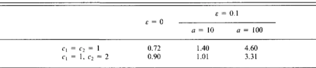
(5.2) F(x) = (l-e-x)(l-e)+l[x>a]-e

This means that given 6 with probability 1 - e a claim is exponential with mean

6 (an ordinary claim) and with probability e it is equal to a • 8 (an outlier

claim). Asymptotic relative efficiences are given in Table 1 for selected values of £ and a. We see that the loss of efficiency in the case e = 0 is more than compensated by cases where large outlier claims are possible. Note that the truncation method of GISLER (1980a, b) cannot handle this situation if Var (0) is not close to zero because the size of the outlying claims is also proportional to d.

TABLE 1

ASYMPTOTIC RELATIVE

ll I

I

EFFICIENCY OF THE ROBUST VERSUS THE LINEAR CREDIBILITY ESTIMATOR IN THE MIXTURE MODEL (5.1)-(5.2)

C 2 = l , c2 1 = 2 £ - 0 0.72 0.90 £ a = 10 1.40 1.01 = 0.1 a = 100 4.60 3.31

5.2. An example with two radically different claim size distributions

In this example the risk parameter and the claim size take only two values:

P[8 = 1] = P[0 = 2] = 0.5,

P[X = 1|0 = 1] = 0.9, P[X = 1O|0 = 1] = 0.1, P[X = 1|0 = 2] = 0, P[X = 1O|0 = 2] = 1.

This means that one group of contracts produces only large claims whereas the first group produces usually small claims with occasional outliers. In this case calculations can be made in closed form without any approximations. The results for n = 10, and c, = c2 = 1 are given in Table 2. We see that the

robust credibility estimator is quite close to the posterior mean which is optimal for square loss — at least in those cases which do occur in practice. The linear credibility estimator is obviously bad. It can be shown easily that the truncation estimator of GISLER (1980a, b) coincides with the linear credibility estimator. It is also instructive to see who pays for the outliers which occur in the first group. It is the lucky person in the same group who has not yet incurred a large claim.

TABLE 2

CREDIBILITY ESTIMATORS IN THE EXAMPLE 5.2 FOR n = 10

Number of claims = 10 0 1 2 3 4 5 10 Probability 0= 1 0.3487 0.3874 0.1937 0.0574 0.0112 0.0015 0 given e = 2 0 0 0 0 0 0 1 1.12 2.00 2.88 3.76 4.64 5.52 9.92 Robust c, = c2 = 1 1.74 1.85 2.04 2.43 3.57 5.86 9.99 Posterior mean 1.9 1.9 1.9 1.9 1.9 1.9 10.0

4 4 HANS R. KONSCH

5.3. An example by GISLER (1980a)

This is again a case where both 0 and X are discrete: 0e{l,2,3,4},

Xe {0, 2, 4, 6, 40}. We have P[6 = i] = 0.25 for all /. The conditional

proba-bilities for X given 6 are given in Table 3. We take n = 3 so that exact calculations can be made without too much work. We compare here four estimators. The first one is the classical linear credibility estimator

/if1 = 3.912 + 0.158 (Xj- 3.912)

The second one is our robust credibility estimator with c, = c2 = 1 and a = a0

given by (4.2):

/ifb = 3.912 + 0.351(7}- 3.089).

The third one is the semilinear credibility estimator with optimal truncation point of GISLER (1980a, b).

/ 1 ^

.794 - £ G(X0)- 2.767

where G(x) = min (x, 4.89). Finally we consider the optimal estimator

g 1 2 3 4 TABLE CONDITIONAL PROBABILITIES JC = 0 0.5445 0.2940 0.0970 0.0480 i x = 2 0.2475 0.2940 0.2910 0.1440 3 ; IN THE EXAMPLE p e[Xi = x] x = 4 0.0990 0.2450 0.3395 0.2880 5.3 JC = 6 0.0990 0.1470 0.2425 0.4800 JC = 40 0.0100 0.0200 0.0300 0.0400

The mean square errors for these estimators are 1.90, 1.47, 1.12 and 1.09. The values of estimators for some realizations of (X^, X2j, X3J) are given in Table 4. We see that typically the robust estimator is between the linear and Gisler's estimator. The most striking exception occurs for contracts with two or three claims of 40. They are heavily charged by our robust estimator. This difference will become irrelevant for somewhat larges «'s because then the probability for a contract to produce a majority of outlier claims is practically zero. Moreover, if we change the model slightly and introduce an additional risk class with Pg [Xtj = 40] ^> 0, then the above bad performance of our estimator turns into an advantage: Whenever there is a majority of outlier claims, we should charge the corresponding contract heavily.

TABLE 4

CREDIBILITY ESTIMATORS IN THE EXAMPLE 5.3 WITH n = 3 AND SELECTED CLAIMS

(X,, X2, X}) (0, 0, 0) (0, 0, 6) (0, 2, 2) (0, 2, 6) (0, 6, 6) (2, 4, 6) (6, 6, 6) (0, 0, 40) (0, 6, 40) (2, 4, 40) (6, 6, 40) (6, 40, 40) Linear 3.29 3.61 3.50 3.72 3.93 3.93 4.24 5.41 5.72 5.72 6.04 7.84 Robust c, = c2 = 1 2.83 2.83 3.30 3.53 4.23 4.23 4.93 2.83 4.93 4.93 7.03 12.86 Gisler 1.72 3.01 2.78 3.54 4.31 4.60 5.60 3.01 4.31 4.60 5.60 5.60 Posterior mean 2.09 2.50 2.78 3.25 4.30 4.69 5.68 2.58 4.13 4.53 5.46 5.58 5.4. Discussion

Our estimator performs well if there are outlying claims and the number of years available is not very small. In other situations it seems to be at least acceptable in its performance. It can deal also well with situations where the outlying claims vary considerably with the risk parameter. The reason for this is that our estimator determines a truncation point separately for each contract, based only on the experience of the contract under consideration. If the number of years is small, one might want to use also the experience from other contracts to some extent. How this can be done in a robust way is the topic of the next section.

6. A MORE SOPHISTICATED APPROACH

We consider first Case I with known distributions and fix a measure z for the average claim size. It could be isfA'], but it is preferable to choose z robust so that it is not affected by single outliers and atypical contracts. A concrete proposal is given below. We then suggest the following estimator

(6.1)

where // = E[Xj] and T is defined implicitly as the solution of (6.2)

Here / ( x ) = m a x ( - c , , m i n ( x - l , c2)) as before. In order to explain the

character of this estimator, consider first the case cx = 1, c2 = oo. Then by a simple calculation T = y (n + y) ~' t + n (« + y) ~' X_ and /T(r?)~ = y (n + y) ~' n +

4 6 HANS R. KUNSCH

n (n + y) ~' X . We thus recover the usual linear credibility estimator with

credibility factor n(n + y)~\ In the general case we introduce the truncated claims

Xr = max ((1 - c,) T, min {X,, (1 + c2) T)).

One then finds by the same argument that

(6.3) T=n(n + yy

n-

£ *,* + y (n + y) ~' r,

i.e. 7" is a convex combination of the a priori value z and the mean of the truncated claims. The truncation point depends however on T (and thus on z and Xx, ..., Xn) so that (6.3) is not an explicit solution. The estimator T incorporates already the a priori value z with the weight y(n + y)~'. The passage from T to /f(9j serves only to achieve unbiasedness; there is no need to introduce an additional credibility factor there.

The main advantage of this proposal is that the a priori value z is used to find the truncation points (1 - c , ) T and (1 + c2) T. This improves the ability of

the estimator to detect and truncate outlying claims. It is most visible when we study the breakdown points of T. With similar arguments as in Section 3.1-2 we can prove the following result.

Lemma 6.1:

i) Equation (6.2) has always a unique solution in the interval

[y{ncx + y)~lx, oo).

ii) T h e b r e a k d o w n point, i.e. the maximal n u m b e r of claims tending to infinity the estimator can tolerate without going to infinity, is given by min {ie IN,

Again a choice cx = 1, c2 between 1 and 2 is expected to work well in most

cases.

A different justification of our estimator T can be obtained from the Bayesian viewpoint. It is easily checked that (6.2) is the normal equation for the estimator maximizing the a posteriori density if we choose F0{dx) = 6~lf(xd~l)dx with

(e~x, x < \+c2

f(x) = const. {

and

U{d6) = const. xy-l8~rexp(-yT/ff)d6

provided cx = 1, c2 > 0, y > 1. We thus see that our proposal corresponds to

parameter. Note that the above prior U means that 9~l ~ Gamma (y — 1, yr). The assumption of scale families for both F and U leads to an estimator which is scale equivariant: If X{,..., Xn and x are multiplied by a constant, then T is multiplied by the same constant.

Next we discuss the choice of the a priori value x. We propose to use the solution of the following equation

\ X(T(0)/T) U{d9) = 0 where x{0) is determined by ' X(x/z(9))F0(dx) =

I

and x is the by now well known truncated linear function. From what has been said before, it is clear that T is a robust measure of the average claim size. The example of the linear credibility estimator at the beginning showed that the choice of x is irrelevant if c, = 1 and c2 = oo. Presumably in other cases too the value of x will not be crucial.

In Case II which is relevant for applications our proposal is as follows (6.4)

(6.5)

(6.6)

(6.7)

This is a straightforward modification of the previous definitions replacing expectations by averages. Note that T, is nothing else than our proposal 7} from Section 2. Arguing like for (2.8), we see that t is the mean of the truncated T/S.

In order to complete our discussion we have to determine y by an objective procedure from the data. We do this by minimizing an estimate of mean square error. In Case I it follows from (6.1) that

1=1

J

(6.8)

= E

[T],fi(e))-4 8 HANS R. KUNSCH

Because T is nonlinear, Ee[T] and Varw |T] are difficult to evaluate. An

approximation can be obtained like in Section 3.3 by linearizing. If y is fixed and n tends to infinity, the influence of z disappears as is easily seen in the example of linear credibility. Hence in order to obtain a nontrivial asymptotics, we take y = y(n) = ny^. Then we obtain by a Taylor expansion (cf. HAMPEL

et al., 1986, Chap. 2):

(6.9) T{Xl,...,Xn;x) = T(6,x) + n-[ £ IF(X,, 6, T) + O > ~ '/ 2)

where T{6,x) is defined implicitly by

(6.10) f x(x/T(e,z))Fg(dx) = yx(l-T/r(0,T))

and the influence function IF is now

(6.11) IF(x, 9, r) = {X(x/T(9, T))-ya>{\-Tin0, T))} T(6, r)2 M(8,

(6.12) with M(9,z)= [ X'(x/T(j9,T))xF0(dx) + ya,T.

Note that E0[IF(Xi,0,T)] = 0. Hence Eo[T] w T(0, T) and Varw(7) «

«~' J /F(x, 5, T)2 F0(dx). This can be plugged into the formula for the mean

square error which then can be minimized with respect to y. Details are left to the reader.

In Case II we need estimates for the different terms on the rightjiand side of (6.8): An unbiased estimator for Var(7) is ( J - l ) "1 S/= 1 (Tj-f)2. Because

(TJ-T.)(XJ-XJ _ J

j

= (J- 1) {Cov (Eg[T], n(0)) + E [Covff/ (Tj, XJ]}

we must estimate also E[Cov0 (Tj, X_t)]. The linearization (6.9)-(6.12) suggests

to do this by J n 7 = 1 1 = 1 where (6.13) fPix, Tj, T) = {x(x/Tj)-yn-l(l-TlTj)}T?M(Tj, and (6.14) M(Tj,x) = «"

Taking all this together we minimize the following expression with respect to y

j

(6.15) (J-\yl X {(TJ-T.)2-2(TJ~T,)(X_J-XJ} +

7 = 1

j = 1 <•= 1

A lengthy but straightforward calculation shows that in the case cx = 1,

c2 = oo IF(x, Tj,x) = n(n + 7)~' ( x - Z7) . Thus (6.15) becomes J J n

x

X (X-X)

(oc

-2a) + 2n-

r

(n-\y' £ £ (X-X)

{J-\)x X (X.j-X.)2 (oc2-2a) + 2n-[rl(n-\y' £ £ (Xg-Xj)2a

7 = 1 7 = 1 ' = 1

where a = n(n + y) '. So in this case the minimization can be done in closed form and gives the classical result. In general we will have to find the optimal y numerically by evaluation of (6.15) for some values of y. Since the exact value of y will not matter too much, a coarse search ought to be sufficient. This completes the presentation of our second proposal.

REFERENCES

EFRON, B. (1982) The Jackknife, lire Bootstrap and Other Resampling Plans. CBMS Regional Conference Series 38. SIAM Philadelphia.

GISLER, A. (1980a) Optimales Stutzen von Beobachtungen im Credibility Modell. Ph. D. thesis, ETH Zurich, Nr. 6556.

GISLER, A. (1980b) Optimum trimming of data in the credibility model. Mitteilungen Ver. Schweiz.,

Vers. math. 80, 313 326.

GISLER, A. and REINHARD, P. (1990) Robust Credibility. Paper presented at the XXIIth Astin Colloquium, Montreux.

HAMPEL, F. R., RONCHETTI, E. M., ROUSSEEUW, P.J. and STAHEL, W.A. (1986) Robust Statistics:

The Approach Based on Influence Functions. Wiley, New York.

HUBER, P. (1981) Robust Statistics. Wiley, New York.

HANS R. KUNSCH