HAL Id: insu-02911744
https://hal-insu.archives-ouvertes.fr/insu-02911744
Submitted on 4 Aug 2020
HAL is a multi-disciplinary open access
archive for the deposit and dissemination of
sci-entific research documents, whether they are
pub-lished or not. The documents may come from
teaching and research institutions in France or
abroad, or from public or private research centers.
L’archive ouverte pluridisciplinaire HAL, est
destinée au dépôt et à la diffusion de documents
scientifiques de niveau recherche, publiés ou non,
émanant des établissements d’enseignement et de
recherche français ou étrangers, des laboratoires
publics ou privés.
To cite this version:
Gaétane Ronsmans, Catherine Wespes, Lieven Clarisse, Susan Solomon, Daniel Hurtmans, et al.. A
nitric acid dataset from IASI for polar stratospheric denitrification studies. Atmospheric Chemistry
and Physics Discussions, European Geosciences Union, 2021, pp.(Under Review).
�10.5194/acp-2020-347�. �insu-02911744�
A nitric acid dataset from IASI for polar stratospheric
denitrification studies
Gaetane Ronsmans
1, Catherine Wespes
1,*, Lieven Clarisse
1, Susan Solomon
2, Daniel Hurtmans
1, Cathy
Clerbaux
1,3, and Pierre-François Coheur
11Université libre de Bruxelles (ULB), Spectroscopy, Quantum Chemistry and Atmospheric Remote Sensing (SQUARES),
Brussels, Belgium
2Department of Earth, Atmospheric and Planetary Sciences, Massachusetts Institute of Technology, Cambridge,
Massachusetts, USA
3LATMOS/IPSL, Sorbonne Université, UVSQ, CNRS, Paris, France
Correspondence: Catherine Wespes ([email protected])
Abstract. In this paper, we exploit the first 10-year data-record (2008-2017) of nitric acid (HNO3) total columns measured by
the IASI-A/Metop infrared sounder, characterized by an exceptional daily sampling and a good vertical sensitivity in the mid-stratosphere (around 50 hPa), to monitor the causal relationship between the temperature decrease and the observed HNO3loss
that occurs each year in the Antarctic stratosphere during the polar night. Since the HNO3depletion results from the formation
of polar stratospheric clouds (PSCs) which trigger the development of the ozone (O3) hole, its continuous monitoring is of high
5
importance. We verify here, from the 10-year time evolution of the pair HNO3-temperature (taken from reanalysis at 50 hPa),
the recurrence of specific regimes in the cycle of IASI HNO3and identify, for each year, the day and the 50 hPa-temperature
("drop temperature") corresponding to the onset of denitrification in Antarctic winter. Although the measured HNO3 total
column does not allow differentiating the uptake of HNO3 by different types of PSC particles along the vertical profile, an
average drop temperature of ∼191 ± 3 K, consistent with the nitric acid trihydrate (NAT) formation temperature (close to 10
195 K at 50 hPa), is found. The spatial distribution and inter-annual variability of the drop temperature are briefly investigated and discussed in the context of previous PSCs studies. This paper highlights the capability of the IASI sounder to monitor the long-term evolution of the polar stratospheric composition and processes involved in the depletion of stratospheric O3.
1 Introduction 15
The cold and isolated air masses found within the polar vortex during winter are associated with a strong denitrification of the stratosphere due to the formation of PSCs (composed of HNO3, sulphuric acid (H2SO4) and water ice (H2O)) (Peter, 1997;
Voigt et al., 2000; von König, 2002; Schreiner et al., 2003). These clouds strongly affect the polar chemistry by (1) acting as surfaces for the heterogeneous activation of chlorine and bromine compounds, in turn leading to enhanced O3destruction
(Solomon, 1999; Wang and Michelangeli, 2006; Harris et al., 2010; Wegner et al., 2012) and by (2) removing gas-phase 20
HNO3temporarily or permanently through uptake by PSCs and sedimentation of large PSC particles to lower altitudes. The
denitrification of the polar stratosphere during winter delays the reformation of chlorine reservoirs and, hence, intensifies the O3 hole (Solomon, 1999; Harris et al., 2010). The heterogeneous reaction rates on PSCs surface and the uptake of HNO3
strongly depend on the temperature and on the PSCs particle type. The PSCs are classified into three different types based on their composition and optical properties: type Ia solid nitric acid trihydrate - NAT (HNO3· (H2O)3), type Ib liquid supercooled
25
ternary solution - STS (HNO3/H2SO4/H2O with variable composition) and type II, crystalline water-ice particles (likely
composed of a combination of different chemical phases) (e.g. (Toon et al., 1986; Koop et al., 2000; Voigt et al., 2000; Lowe and MacKenzie, 2008)). In the stratosphere, they mostly consist of mixtures of liquid/solid STS/NAT particles in varying number densities, with HNO3 being the major constituent of these particles. The large-size NAT particles of low number
density are the principal cause of sedimentation(Lambert et al., 2012; Pitts et al., 2013; Molleker et al., 2014; Lambert et al., 30
2016). The formation temperature of STS (TST S) and the thermodynamic equilibrium temperatures of NAT (TN AT) and ice
(Tice), have been determined, respectively, as: ∼ 192 K (Carslaw et al., 1995), ∼ 195.7 K (Hanson and Mauersberger, 1988)
and ∼ 188 K (Murphy and Koop, 2005) for typical 50 hPa atmospheric conditions (5 ppmv H2O and 10 ppbv HNO3). While
the NAT nucleation was thought to require temperature below Tice and pre-existing ice particles, recent observational and
modelling studies have shown that HNO3starts to condense in early PSC season in liquid NAT mixtures well above Tice(∼
35
4 K below TN AT, close to TST S) even after a very short temperature threshold exposure (TTE) to these temperatures but also
slightly below TN AT after a long TTE, whereas the NAT existence persists up to TN AT (Pitts et al., 2013; Hoyle et al., 2013;
Lambert et al., 2016; Pitts et al., 2018). It has been recently proposed that the higher temperature condensation results from heterogeneous nucleation of NAT on meteoritic dust in liquid aerosol (Hoyle et al., 2013; Grooß et al., 2014; James et al., 2018). Further cooling below TST S and Tice leads to nucleation of liquid STS, of solid NAT onto ice and of ice particles
40
mainly from STS (type II PSCs) (Lowe and MacKenzie, 2008). The formation of NAT and ice has also been shown to be triggered by stratospheric mountain-waves (Carslaw et al., 1998; Hoffmann et al., 2017). Altough the formation mechanisms and composition of STS droplets in stratospheric conditions are well described (Toon et al., 1986; Carslaw et al., 1995; Lowe and MacKenzie, 2008), the NAT and ice nucleation processes still require further investigation. This could be important as the chemistry-climate models (CCMs) generally oversimplify the heterogeneous nucleation schemes for the PSCs formation (Zhu 45
et al., 2015; Spang et al., 2018; Snels et al., 2019) preventing an accurate estimation of O3levels. The influence of HNO3in
modulating O3abundances in the stratosphere is furthermore underrepresented in CCMs (Kvissel et al., 2012).
Several satellite instruments measure stratospheric HNO3 (MLS/Aura (Santee et al., 2007), MIPAS/ENVISAT (Piccolo
and Dudhia, 2007), ACE-FTS/SCISAT (Sheese et al., 2017) and SMR/Odin (Urban et al., 2009)). The spaceborne lidars CALIOP/CALIPSO and the infrared instrument MIPAS/Envisat) are capable to detect and classify the PSC types, and to fol-50
low their formation mechanisms (e.g. (Lambert et al., 2016; Pitts et al., 2018; Spang et al., 2018) and references therein), which complements in situ measurements (Voigt et al., 2005) and ground-based lidar (Snels et al., 2019). From these available observational datasets, the HNO3 depletion has been linked to the PSCs formation and detected below the TN AT threshold
fur-ther investigation given the complexity of the nucleation mechanisms that depends on a series of parameters (e.g. atmospheric 55
temperature, water and HNO3vapour pressure, time exposure to temperatures, temperature history).
In contrast to the limb satellite instruments mentioned above, the infrared nadir sounder IASI offers a dense spatial sampling of the entire globe, twice a day (Section 2). While it cannot provide a vertical profile of HNO3similar to the limb sounders,
IASI provides reliable total column measurements of HNO3 with a maximum sensitivity in the mid-stratosphere around 50
hPa (Ronsmans et al., 2016, 2018) where the PSCs cloud form (Voigt et al., 2005; Lambert et al., 2012; Spang et al., 2016, 60
2018). This study aims to explore the 10-years continuous HNO3measurements from IASI for providing a long-term global
picture of denitrification and of its dependence to temperatures during polar winter (Section 3). The temperature corresponding to the onset of the strong depletion in HNO3records (here referred to as ‘drop temperature’) is identified in Section 4 for each
observed year and discussed in the context of previous studies. 2 Data
65
The HNO3data used in the present study are obtained from measurements of the Infrared Atmospheric Sounding
Interferom-eter (IASI) embarked on the Metop-A satellite. IASI measures the Earth’s and atmosphere’s radiation in the thermal infrared spectral range (645 − 2760 cm−1), with a 0.5 cm−1apodized resolution and a low radiometric noise (Clerbaux et al., 2009;
Hilton et al., 2012). Thanks to its polar sun-synchronous orbit with more than 14 orbits a day and a field of view of four si-multaneous footprints of 12 km at nadir, IASI provides global coverage twice a day (9.30 AM and PM mean local solar time). 70
That extensive spatial and temporal sampling in the polar regions is key to this study.
The HNO3vertical profiles are retrieved on a uniform vertical 1 km grid of 41 layers (from the surface to 40 km with an
extra layer above to 60 km) in near-real-time by the Fast Optimal Retrieval on Layers for IASI (FORLI) software, using the optimal estimation method (Rodgers, 2000). Detailed information on the FORLI algorithm and retrieval parameters specific to HNO3can be found in previous papers (Hurtmans et al., 2012; Ronsmans et al., 2016). For this study, only the total columns
75
(v20151001) are used, considering (1) the low vertical sensitivity of IASI with only one independent piece of information, (2) the limited sensitivity of IASI to tropospheric HNO3, (3) the dominant contribution of the stratosphere to the HNO3total
column and (4) the largest sensitivity of IASI is the region of interest, i.e. in the mid-stratosphere (from ∼10 to ∼30 km), where the HNO3abundance is the highest (Ronsmans et al., 2016). The total columns yield a total retrieval error of 10% and a low
bias (10.5 %) compared to ground-based FTIR measurements (Hurtmans et al., 2012; Ronsmans et al., 2016). Quality flags 80
similar to those developed for O3in previous IASI studies (Wespes et al., 2017) were applied a posteriori to exclude data (i)
with a corresponding poor spectral fit, (ii) with less reliability or (iii) with cloud contamination (defined by a fractional cloud cover ≥ 25 %). Note that the HNO3 total column distributions illustrated in sections below use the median as a statistical
average since it is more robust against the outliers than the normal mean.
Temperature and potential vorticity (PV) fields are taken from the ECMWF ERA Interim Reanalysis dataset, respectively 85
at 50 hPa and at the potential temperature of 530 K (corresponding to ∼ 20 km altitude where the IASI sensitivity to HNO3
below TN AT (∼ 195.7 K at 50 hPa (Hanson and Mauersberger, 1988)) depending on the meteorological conditions (Pitts et al.,
2013; Hoyle et al., 2013; Lambert et al., 2016; Pitts et al., 2018), a threshold temperature of 195 K is considered in the sections below to identify the PSCs-containing regions. The potential vorticity is used to delimit dynamically consistent areas in the 90
polar regions. In what follows, we use either the equivalent latitudes ("eqlat", calculated from PV fields at 530 K) or the PV values to characterize the relationship between HNO3and temperatures in the cold polar regions. Uncertainties in ERA-Interim
temperatures will also be discussed below. 3 Annual cycle of HNO3vs temperatures
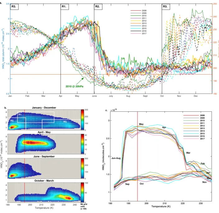
Figure 1a shows the yearly HNO3 cycle (solid lines, left axis) in the southernmost equivalent latitudes (70◦− 90◦ S), as
95
measured by IASI over the whole period of measurements (2008–2017). The total HNO3variability in such equivalent latitudes
has already been discussed in a previous IASI study (Ronsmans et al., 2018) where the contribution of the PSCs into the HNO3
variations was highlighted. The temperature time series, taken at 50 hPa, is here represented as well (dashed lines, right axis). From this figure, different regimes of HNO3total columns vs temperature can be observed throughout the year and from one
year to another. In particular, we define here three main regimes (R1, R2 and R3) along the HNO3cycle. The full cycle and
100
the main regimes in the 70◦− 90◦S eqlat region are further represented in Fig. 1b that shows a histogram of the HNO 3total
columns as a function of temperature for the year 2011. The red vertical line in Fig. 1a and Fig. 1b represent the 195 K threshold temperature used to identify the onset of HNO3uptake by PSCs (see Section 2). The three identified regimes correspond to:
- R1 is defined by the maxima in the total HNO3abundances covering the months of April and May (∼ 3×10¹⁶molec.cm−2,
R1 in Figure 1a and b), when the 50 hPa temperature strongly decreases (from ∼220 to ∼195 K). These high HNO3
105
levels result from low sunlight, preventing photodissociation, along with the heterogeneous hydrolysis of N2O5Santee
et al. (1999); Urban et al. (2009); de Zafra and Smyshlyaev (2001).
- R2 which extents from June to September is characterized by the onset of the strong decrease in HNO3total columns at the
beginning of June, when the temperatures fall below 195 K, followed by a plateau of total HNO3minima. In this regime,
the HNO3total columns average below 2 × 10¹⁶molec.cm−2 and the 50 hPa temperatures range mostly between 180
110
and 190 K.
- R3 starts in October when sunlight returns and the 50 hPa temperatures rise above 195 K. Despite the stratospheric warming with 50 hPa temperatures up to 240 K in summer, the HNO3total columns stagnate at the R2 plateau levels (around 1.5×
1016molec.cm−2). This regime likely reflects the photolysis of NO
3and HNO3itself (Ronsmans et al., 2018) as well as
the permanent denitrification of the mid-stratosphere, caused by the PSCs sedimentation, despite the renitrification of the 115
lowermost stratosphere (Braun et al., 2019) where the IASI sensitivity to HNO3is lower (Ronsmans et al., 2016). The
plateau lasts until approximately February, where HNO3total column slowly starts increasing, reaching the April-May
Jan Feb Mar Apr May June July Aug Sept Oct Nov Dec 0.5 1 1.5 2 2.5 3 3.5 HNO 3 total column (10 16 molec.cm -2) 180 190 200 210 220 230 240 250 Temperature (K) 2008 2009 2010 2011 2012 2013 2014 2015 2016 2017 a. R3. R1. R2. R3. 2010 @ 20hPa 1 2 3 4 January - December 0 100 200 300 1 2 3 4 April - May 0 10 20 30 40 1 2 3 4 HNO 3 (10 16 molec.cm -2) June - September 0 100 200 300 180 190 200 210 220 230 240 Temperature (K) 1 2 3 4 October - March 0 50 100 b. Nb grid cells (x 100) R1. R2. R3. 180 190 200 210 220 230 Temperature (K) 1 1.5 2 2.5 3 HNO 3 (molecules.cm -2) 1016 Jan Feb Mar Apr May Jun-Aug
Sep Oct Nov
Dec 2008 2009 2010 2011 2012 2013 2014 2015 2016 2017 c.
Figure 1. (a) Time series of daily averaged HNO3 total columns (solid lines) and temperatures taken at 50 hPa (dashed lines) at the
70◦− 90◦S equivalent latitudes, for the years 2008–2017. The green dotted line represents the temperatures at 20 hPa for the year 2010. (b)
HNO3total columns versus temperatures (at 50 hPa) histogram for the whole year (top) and for the 3 defined regimes (R1 - R3) separated
in (a) for the year 2011. The colors refer to the number of measurements in each cell. (c) Evolution of daily averaged HNO3total columns
As illustrated in Fig. 1a, the three regimes are observed each year with, however, some interannual variations. For instance, the sudden stratospheric warming (SSW) that occurs in 2010 (see the temperature time series at 20 hPa for the year 2010; 120
green dotted line) yielded higher HNO3total columns (see green solid line in July and August) (de Laat and van Weele, 2011;
Klekociuk et al., 2011; WMO, 2014; Ronsmans et al., 2018).
Figure 1c shows the evolution of the relationship between the daily averaged HNO3 (calculated from a 7-days moving
average) with the highest occurrence (in the range of 0.1 ×10¹⁶molec.cm−2) and the 50 hPa temperature, over the 10 years of
IASI. It clearly illustrates the slow increase in HNO3columns as the temperatures decrease (February to May, i.e. R3 to R1),
125
the strong and rapid HNO3depletion in June (R1 to R2), the plateau of low HNO3abundances in winter and spring (from
August to November; R2 to R3). Figure 1c also highlights the interannual variability in total HNO3, which is found to be the
largest in R3, and shows a strong consistency in the onset of the depletion between each year (beginning of June when the temperatures fall below 195 K as indicated by the red vertical line). Fig. 1c is accompanied by an animation, provided in the Supplementary material, showing the daily evolution of the histogram of the HNO3total columns as a function of the 50 hPa
130
temperature, averaged in a 7-days windows over all the years. Given the span of PSCs formation over a large range of altitudes (typically between 10 and 30 km) (Höpfner et al., 2006, 2009; Spang et al., 2018; Pitts et al., 2018) and that of maximum IASI sensitivity to HNO3 around 50 hPa (Hurtmans et al., 2012; Ronsmans et al., 2016), the temperatures at two other pressure
levels, namely 70 and 30 hPa (i.e. ∼15 and ∼25 km), have also been tested to investigate the relationship between HNO3
and temperature in the mid-stratosphere. The results (not shown here) exhibit a similar HNO3-temperature behavior at the
135
different levels with, as expected, lower and larger temperatures in R2, respectively, at 30 hPa (180 and 185 K) and at 70 hPa (∼190 K), but still below the NAT formation threshold at these pressure levels (TN AT∼193 K at 30 hPa and ∼197 K at 70 hPa)
(Lambert et al., 2016). Therefore, the altitude range of maximum IASI sensitivity to HNO3 (see Section 2) is characterized
by the PSCs formation and the denitrification process. Furthermore, the consistency between the 195 K threshold temperature taken at 50 hPa and the onset of the strong total HNO3depletion seen in IASI data (see Fig. 1a and Fig. 1c) is in agreement
140
with the largest NAT area that starts to develop in June around 20 km (Spang et al., 2018), which justifies the use of the 195 K temperature at that single representative level in this study. Despite the limited vertical resolution of IASI which does not allow to investigate the HNO3uptake by the different types of PSCs during their formation and growth along the vertical profile, the
HNO3total column measurements from IASI constitute an important new dataset for exploring the polar denitrification over
the whole stratosphere. This is particularly relevant considering the mission continuity, which will span several decades with 145
the planned follow-on missions.
4 Onset of HNO3depletion and drop temperature detection
To go beyond the vertically integrated view of denitrification and to identify its spatial and temporal variability, the daily time evolution of HNO3during the first 10 years of IASI measurements and the temperatures at 50 hPa are explored. In particular,
the second derivative of HNO3total column with respect to time is calculated to detect the strongest rate of decrease seen in
150
Jan08
06Jun08 Jan09 10Jun09 Jan10 17May10 Jan11
20May11 Jan12
08Jun12 Jan13 17May13 Jan14
23May14 Jan15 20May15 Jan16
04Jun16 Jan17 17May17
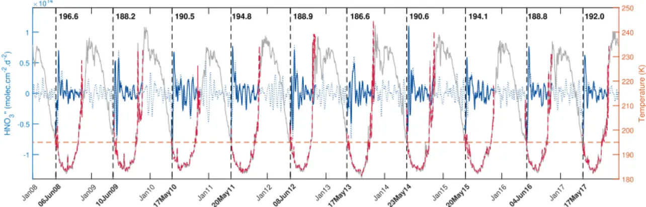
-1 -0.5 0 0.5 1 HNO 3 " (molec.cm -2.d -2) 1014 180 190 200 210 220 230 240 250 Temperature (K) 196.6 188.2 190.5 194.8 188.9 186.6 190.6 194.1 188.8 192.0
Figure 2. Time series of total HNO3second derivative (blue, left y-axis) and of the temperature (red, right y-axis), in the region of potential
vorticity lower than −10 ×10−5K.m2.kg−1.s−1. The red horizontal line corresponds to the 195 K temperature. The vertical dashed lines
indicate the second derivative minimum in HNO3 for each year. The corresponding dates (in bold, on the x-axis) and temperatures also
are indicated. The time series of total HNO3second derivative (dashed blue) and of temperature (grey) in the70–90◦S Eqlat band are also
represented.
4.1 HNO3vs temperature time series
Figure 2 shows the time series of the second derivative of HNO3total column with respect to time (blue) and of the temperature
(red) averaged in the areas of potential vorticity smaller than −10×10-5K.m2.kg-1.s-1to encompass the regions inside the inner
polar vortex where the temperatures and the total HNO3depletion are the coldest (Ronsmans et al., 2018). The use of that PV
155
threshold value explains the gaps in the time series during the summer when the PV does not reach such low levels, while the time series averaged in the 70◦- 90◦S Eqlat band (dashed blue for the second derivative of HNO
3and grey for the temperature)
covers the full year.
Note that the HNO3time series has been smoothed with a simple spline data interpolation function to avoid gaps before
calculating the second derivative of HNO3total column with respect to time as the daily second-difference HNO3total column.
160
The horizontal red line shows the 195 K threshold. As already illustrated in Fig. 1a and Fig. 1c, the strongest rate of HNO3
depletion (i.e. the second derivative minimum) is found around the 195 K threshold temperature, within a few days (4 to 23 days) after total HNO3reaches its maximum, i.e. typically between the 17thof May (2010, 2013 and 2017) and the 10thof June
(2009). The 50 hPa drop temperature are detected between 188.2 K and 196.6 K, with an average of 191.1±3.2 K (1σ standard deviation) over the ten years. Knowing that TN AT can be higher or lower depending on the atmospheric conditions and that
165
NAT starts to nucleate from ∼2–4 K below TN AT (Pitts et al., 2011; Hoyle et al., 2013; Lambert et al., 2016), the results here
demonstrate the consistency between the 50 hPa drop temperature, i.e. the temperature associated with the strongest HNO3
depletion detected from IASI, and the PSCs occurrence in the mid-stratosphere at polar latitudes. It further justifies the use of the single 50 hPa level for characterizing and investigating the onset of HNO3denitrification from IASI.
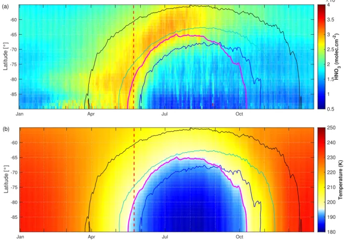
Jan Apr Jul Oct -85 -80 -75 -70 -65 -60 Latitude [°] 0.5 1 1.5 2 2.5 3 3.5 4 HNO 3 (molec.cm -2) 1016
Jan Apr Jul Oct
-85 -80 -75 -70 -65 -60 Latitude [°] 180 190 200 210 220 230 240 250 Temperature (K) (b) (a)
Figure 3. Zonal distributions of (a) HNO3total columns (in molec.cm-2) from IASI and (b) temperatures at 50 hPa from ERA Interim (in K)
between 55◦to 90◦south and averaged over the years 2008–2017. Three isocontours for PV of −5 (black), −8 (cyan) and −10 (blue) (in
×10-5K.m2.kg-1.s-1) and one isocontour for the 195 K temperature at 50 hPa (pink) are sumperimposed. The vertical red dashed line indicates,
at 90◦S, the 10-year average of the drop temperatures calculated from the HNO3 time series second derivative in the area delimited by a
−10×10-6K.m2.kg-1.s-1PV contour.
Figure 3a and b show the zonal distribution of HNO3 total columns and of the temperature at 50 hPa, respectively,
span-170
ning 55◦-90◦S over the whole IASI period, with, superimposed, three isocontours levels of potential vorticity (−10, −8 and
−5×10⁻⁵K.m2.kg-1.s-1in blue, cyan and black, respectively) and one isocontour for the 50 hPa temperature. The PV
isocon-tour of −10 ×10−5K.m2.kg−1.s−1is clearly shown to separate well the region of strong depletion in total HNO
3according
to the latitude and the time. The red vertical dashed lines indicates, at 90◦S, the average of the drop temperatures calculated in
the area of PV −10 ×10−5K.m2.kg−1.s−1 (191.1 ± 3.2 K; see Fig. 2) over the IASI period. It shows that the strongest rate
175
in HNO3depletion occurs on average a few days before June. The delay of 4–23 days between the maximum in total HNO3
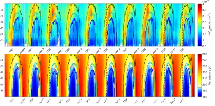
and the start of the depletion (see Fig. 2) is also visible in Fig. 3a. The yearly zonally averaged time series over the ten years of IASI can be found in Fig. 4; it shows the reproducibility in the HNO3depletion measured from IASI from year to year.
Figure 4. Zonally averaged distributions of (top) HNO3 total columns (in molec.cm-2) from IASI and (bottom) temperatures at 50 hPa
from ERA Interim (in K). The latitude range is from 55◦to 90◦south, and the isocontours are PVs of -5 (black), -8 (cyan) and -10 (blue)
(in ×10-5 K.m2.kg-1.s-1). The vertical red dashed lines correspond to the second derivative minima each year in the area delimited by a
−10×10-5K.m2.kg-1.s-1PV contour.
4.2 Distribution of drop temperatures
To explore the capability of IASI to monitor the onset of denitrification at a large scale from year to year, Figure 5 shows the 180
spatial variability of the drop 50 hPa temperatures (based on the second derivative minima of total HNO3averaged in 1◦× 1◦
grid cells) inside a PV region of ≤ −8× 10⁻⁵K.m2.kg−1.s−1, for each year of the IASI period. The red contour represents the
PV isocontour of ≤ −10× 10−5K.m2.kg−1.s−1 that delimits our region of interest. The dates corresponding to the onset of
HNO3depletion inside that region are found to range between mid-May and early-July (not shown here). The calculated drop
temperatures vary significantly between ∼ 180 and ∼ 210 K. These high extremes are only found in very few cases and should 185
be considered with caution as they correspond to specific regions above ice shelves with emissivity features that are known to yield errors in the IASI retrievals (Hurtmans et al., 2012; Ronsmans et al., 2016). Note also that these spatial variations might partly reflect the range of maximum sensitivity of IASI to HNO3 (hence, the use of temperature at a single pressure level
might be restrictive to some extent) and biases in ECMWF reanalysis. Reanalysis data sets are, indeed, known to feature large uncertainties. In particular, they do not always capture small-scale fluctuations due to the limited spatial resolution, especially in 190
the south polar regions. Nevertheless, the uncertainties are reduced for several years, thanks to the assimilation of an advanced Tiros Operational Vertical Sounder (ATOVS) around 1998–2000 in reanalyses, to the better coverage of satellite instruments
2008
2009
2010
2011
2012
2013
2014
2015
2016
2017
190 200 210 220 Temperature (K)Figure 5. Spatial distribution (1◦× 1◦) of the drop temperature at 50 hPa (K) (calculated from the total HNO
3second derivative minima)
for each year of IASI (2008–2017), in a region defined by a PV of ≤ −8× 10⁻⁵K.m2.kg−1.s−1. The red lines represented the isocontour
PV of −10×10-5K.m2.kg-1.s-1averaged over the period 15.05–15.10 for each year.
and to the use of global navigation satellite system (GNSS) radio occultation (RO) (Schreiner et al., 2007; Wang et al., 2007; Lambert and Santee, 2018; Lawrence et al., 2018). Comparisons of the ECMWF ERA Interim dataset used in this work with the COSMIC data (Lambert and Santee, 2018) found a small warm bias, with median differences around 0.5 K, reaching 195
0–0.25 K in the southernmost regions of the globe at ∼ 68–21 hPa where PSCs form. Overall, despite these limitations, the spatial variability in the drop 50 hPa temperatures for IASI total HNO3 is well in agreement with the natural variation in
PSCs nucleation temperatures (from around 3-4 K below the ice frost point - Tice - to slightly below TN AT depending on
atmospheric conditions, on TTE, on the type of formation mechanisms (Pitts et al., 2011; Peter and Grooss, 2012; Hoyle et al., 2013)). It underlines well the benefit of the excellent spatial and temporal coverage of IASI that allows to capture the rapid and 200
5 Conclusions
In this paper, we have explored the added value of the dense HNO3total columns dataset provided by the IASI/Metop satellite
over a full decade (2008–2017) for monitoring the stratospheric denitrification phase that occurs each year in the S.H. and for in-vestigating its relationship to stratospheric temperature, hence, to PSCs occurrence of PSCs. To that end, we focused on and de-205
limited the coldest polar region of the S.H. using a specific PV value at 530 K (∼50 hPa, PV of ≤ −10× 10−5K.m2.kg−1.s−1)
and stratospheric temperatures at 50 hPa, taken from the ECMWF ERA Interim reanalysis. That single representative pressure level has been considered in this study given the maximum sensitivity of IASI to HNO3around that level over a range where
the PSCs formation/denitrification process occur.
The annual cycle of total HNO3, as observed from IASI, has first been characterized according to the temperature evolution.
210
Three various regimes (R1 to R3) in the total HNO3- 50 hPa temperature relationship were highlighted from the time series
over the S.H. polar region and described along the cycle: R1 is defined at play during April and May and characterized by a rapid decrease in 50 hPa temperatures while HNO3 accumulates in the poles; R2, from June to September, shows the onset
of the depletion when the 50 hPa temperatures fall below 195 K (considered here as the onset of PSCs nucleation phase at that level), with a strong consistency between each year; R3, defined from November until March when total HNO3remains
215
at low R2 plateau levels, despite the return of sunlight and heat, characterizes the strong denitrification of the stratosphere, likely due to PSCs sedimentation at lower levels where the IASI sensitivity is low. For each year over the IASI period, the use of the second derivative of the HNO3column versus time was then found particularly valuable to detect the onset of the
HNO3condensation to PSCs. It is captured, on average from IASI, a few days before June with a delay of 4–23 days after the
maximum in total HNO3. The corresponding temperatures (’drop temperatures’) were detected between 188.2 K and 196.6
220
K (191±3 K on average over the 10 years), which demonstrated the good consistency between the 50 hPa drop temperature and the PSCs formation temperatures in that altitude region. Finally, the annual and spatial variability (within 1◦× 1◦) in the
drop temperature was further explored from IASI total HNO3and shown to range between ∼180 and ∼210 K. While recurrent
patterns of extreme high drop temperatures were found from year to year and suspected to result from unfiltered poor quality retrievals in case of emissivity issues above ice, the range of drop temperatures is interestingly found in line with the PSCs 225
nucleation temperature that is known, from previous studies, to strongly depend on a series a factors (e.g. meteorological conditions, HNO3 vapour pressure, temperature threshold exposure, presence of meteoritic dust). The results of this study
highlighted the ability of IASI to measure the variations in total HNO3 and, in particular, to capture and monitor the rapid
denitrification phase over the whole polar regions.
To the best of our knowledge, it is the first time that such a large satellite observational data set of stratospheric HNO3
230
concentrations is exploited to monitor the evolution HNO3versus temperatures. Thanks to the three successive instruments
(IASI-A launched in 2006 and still operating, IASI-B in 2012, and IASI-C in 2018) that demonstrate an excellent stability of the Level-1 radiances, the measurements will soon provide an unprecedented long-term dataset of HNO3total columns. It could
could also make use of this unique data set to investigate the relation between HNO3, O3, and meteorology in the changing
235
climate.
Data availability. The IASI HNO3data processed with FORLI-HNO3v0151001 are available upon request to the corresponding author.
Author contributions. G.R. performed the analysis, wrote the manuscript and prepared the figures. C.W. and L.C. contributed to the analysis. C.W., S.S., P.-F. C. and L.C. contributed to the interpretation of the results. D.H. was responsible for the retrieval algorithm development and the processing of the IASI HNO3dataset. All authors contributed to the writting of the text and reviewed the manuscript.
240
Competing interests. The authors declare no competing interests.
Acknowledgements. IASI has been developed and built under the responsibility of the Centre National d’Etudes Spatiales (CNES, France). It is flown on board the Metop satellites as part of the EUMETSAT Polar System. The IASI L1 data are received through the EUMETCast near-real-time data distribution service. The research was funded by the F.R.S.-FNRS, the Belgian State Federal Office for Scientific, Tech-nical and Cultural Affairs (Prodex arrangement 4000111403 IASI.FLOW) and EUMETSAT through the Satellite Application Facility on
245
Atmospheric Composition Monitoring (ACSAF). G. Ronsmans is grateful to the Fonds pour la Formation à la Recherche dans l’Industrie et dans l’Agriculture of Belgium for a PhD grant (Boursier FRIA). L. Clarisse is a research associate supported by the F.R.S.-FNRS. C. Clerbaux is grateful to CNES for financial support. S. Solomon is supported by the National Science Foundation (NSF-1539972).
References
Braun, M., Grooß, J.-U., Woiwode, W., Johansson, S., Höpfner, M., Friedl-Vallon, F., Oelhaf, H., Preusse, P., Ungermann, J., Sinnhuber,
250
B.-M., Ziereis, H., and Braesicke, P.: Nitrification of the lowermost stratosphere during the exceptionally cold Arctic winter 2015/16, Atmospheric Chemistry and Physics Discussions, https://doi.org/10.5194/acp-2019-108, 2019.
Carslaw, K. S., Luo, B. P., and Peter, T.: An analytical expression for the composition of aqueous {HNO_3-H_2SO_4-H_2O} stratospheric aerosols including gas phase removal of {HNO_3}, Geophys. Res. Lett., 22, 1877–1880, https://doi.org/10.1029/95GL01668, 1995. Carslaw, K. S., Wirth, M., Tsias, A., Luo, B. P., Dörnbrack, A., Leutbecher, M., Volkert, H., Renger, W., Bacmeister, J. T., Reimer,
255
E., and Peter, T.: Increased stratospheric ozone depletion due to mountain-induced atmospheric waves, Nature, 391, 675–678, https://doi.org/10.1038/35589, 1998.
Clerbaux, C., Boynard, A., Clarisse, L., George, M., Hadji-Lazaro, J., Herbin, H., Hurtmans, D., Pommier, M., Razavi, A., Turquety, S., Wespes, C., and Coheur, P.-F.: Monitoring of atmospheric composition using the thermal infrared IASI/MetOp sounder, Atmospheric Chemistry and Physics, 9, 6041–6054, https://doi.org/10.5194/acp-9-6041-2009, 2009.
260
de Laat, A. T. J. and van Weele, M.: The 2010 Antarctic ozone hole: Observed reduction in ozone destruction by minor sudden stratospheric warmings, Scientific Reports, 1, 38, https://doi.org/10.1038/srep00038, 2011.
de Zafra, R. and Smyshlyaev, S. P.: On the formation of HNO3 in the Antarctic mid to upper stratosphere in winter, Journal of Geophysical Research, 106, 23 115, https://doi.org/10.1029/2000JD000314, 2001.
Grooß, J. U., Engel, I., Borrmann, S., Frey, W., Günther, G., Hoyle, C. R., Kivi, R., Luo, B. P., Molleker, S., Peter, T., Pitts, M. C., Schlager,
265
H., Stiller, G., Vömel, H., Walker, K. a., and Müller, R.: Nitric acid trihydrate nucleation and denitrification in the Arctic stratosphere, Atmospheric Chemistry and Physics, 14, 1055–1073, https://doi.org/10.5194/acp-14-1055-2014, 2014.
Hanson, D. and Mauersberger, K.: Laboratory studies of the nitric acid trihydrate: Implications for the south polar stratosphere, Geophysical Research Letters, 15, 855–858, https://doi.org/10.1029/GL015i008p00855, 1988.
Harris, N. R. P., Lehmann, R., Rex, M., and von der Gathen, P.: A closer look at Arctic ozone loss and polar stratospheric clouds, Atmospheric
270
Chemistry and Physics, 10, 8499–8510, https://doi.org/10.5194/acp-10-8499-2010, 2010.
Hilton, F., Armante, R., August, T., Barnet, C., Bouchard, A., Camy-Peyret, C., Capelle, V., Clarisse, L., Clerbaux, C., Coheur, P.-F., Collard, A., Crevoisier, C., Dufour, G., Edwards, D., Faijan, F., Fourrié, N., Gambacorta, A., Goldberg, M., Guidard, V., Hurtmans, D., Illingworth, S., Jacquinet-Husson, N., Kerzenmacher, T., Klaes, D., Lavanant, L., Masiello, G., Matricardi, M., McNally, A., Newman, S., Pavelin, E., Payan, S., Péquignot, E., Peyridieu, S., Phulpin, T., Remedios, J., Schlüssel, P., Serio, C., Strow, L., Stubenrauch, C., Taylor, J., Tobin,
275
D., Wolf, W., and Zhou, D.: Hyperspectral Earth Observation from IASI: Five Years of Accomplishments, Bulletin of the American Meteorological Society, 93, 347–370, https://doi.org/10.1175/BAMS-D-11-00027.1, 2012.
Hoffmann, L., Spang, R., Orr, A., Alexander, M. J., Holt, L. A., and Stein, O.: A decadal satellite record of gravity wave activ-ity in the lower stratosphere to study polar stratospheric cloud formation, Atmospheric Chemistry and Physics, 17, 2901–2920, https://doi.org/10.5194/acp-17-2901-2017, 2017.
280
Höpfner, M., Luo, B. P., Massoli, P., Cairo, F., Spang, R., Snels, M., Di Donfrancesco, G., Stiller, G., von Clarmann, T., Fischer, H., and Biermann, U.: Spectroscopic evidence for NAT, STS, and ice in MIPAS infrared limb emission measurements of polar stratospheric clouds, Atmospheric Chemistry and Physics, 6, 1201–1219, https://doi.org/10.5194/acp-6-1201-2006, 2006.
Höpfner, M., Pitts, M. C., and Poole, L. R.: Comparison between CALIPSO and MIPAS observations of polar stratospheric clouds, Journal of Geophysical Research Atmospheres, 114, 1–15, https://doi.org/10.1029/2009JDO12114, 2009.
Hoyle, C. R., Engel, I., Luo, B. P., Pitts, M. C., Poole, L. R., Grooß, J. U., and Peter, T.: Heterogeneous formation of polar stratospheric clouds-Part 1: Nucleation of nitric acid trihydrate (NAT), Atmospheric Chemistry and Physics, 13, 9577–9595, https://doi.org/10.5194/acp-13-9577-2013, 2013.
Hurtmans, D., Coheur, P.-F., Wespes, C., Clarisse, L., Scharf, O., Clerbaux, C., Hadji-Lazaro, J., George, M., and Turquety, S.: FORLI radiative transfer and retrieval code for IASI, Journal of Quantitative Spectroscopy and Radiative Transfer, 113, 1391–1408,
290
https://doi.org/10.1016/j.jqsrt.2012.02.036, 2012.
James, A. D., Brooke, J. S. A., Mangan, T. P., Whale, T. F., Plane, J. M. C., and Murray, B. J.: Nucleation of nitric acid hydrates in polar stratospheric clouds by meteoric material, Atmospheric Chemistry and Physics, 18, 4519–4531, https://doi.org/10.5194/acp-18-4519-2018, 2018.
Klekociuk, A., Tully, M., Alexander, S., Dargaville, R., Deschamps, L., Fraser, P., Gies, H., Henderson, S., Javorniczky, J., Krummel, P.,
Pe-295
telina, S., Shanklin, J., Siddaway, J., and Stone, K.: The Antarctic ozone hole during 2010, Australian Meteorological and Oceanographic Journal, 61, 253–267, https://doi.org/10.22499/2.6104.006, 2011.
Koop, T., Luo, B., Tsias, A., and Peter, T.: Water activity as the determinant for homogeneous ice nucleation in aqueous solutions, Nature, 406, 611–614, https://doi.org/10.1038/35020537, 2000.
Kvissel, O.-K., Orsolini, Y. J., Stordal, F., Isaksen, I. S. A., and Santee, M. L.: Formation of stratospheric nitric acid by a hydrated ion
300
cluster reaction: Implications for the effect of energetic particle precipitation on the middle atmosphere, Journal of Geophysical Research: Atmospheres, 117, n/a–n/a, https://doi.org/10.1029/2011jd017257, 2012.
Lambert, A. and Santee, M. L.: Accuracy and precision of polar lower stratospheric temperatures from reanalyses evaluated from A-Train CALIOP and MLS, COSMIC GPS RO, and the equilibrium thermodynamics of supercooled ternary solutions and ice clouds, Atmospheric Chemistry and Physics, 18, 1945–1975, https://doi.org/10.5194/acp-18-1945-2018, 2018.
305
Lambert, A., Santee, M. L., Wu, D. L., and Chae, J. H.: A-train CALIOP and MLS observations of early winter Antarctic polar stratospheric clouds and nitric acid in 2008, Atmospheric Chemistry and Physics, 12, 2899–2931, https://doi.org/10.5194/acp-12-2899-2012, 2012. Lambert, A., Santee, M. L., and Livesey, N. J.: Interannual variations of early winter Antarctic polar stratospheric cloud formation and nitric
acid observed by CALIOP and MLS, Atmospheric Chemistry and Physics, 16, 15 219–15 246, https://doi.org/10.5194/acp-16-15219-2016, 2016.
310
Lawrence, Z. D., Manney, G. L., and Wargan, K.: Reanalysis intercomparisons of stratospheric polar processing diagnostics, Atmospheric Chemistry and Physics, 18, 13 547–13 579, https://doi.org/10.5194/acp-18-13547-2018, 2018.
Lowe, D. and MacKenzie, A. R.: Polar stratospheric cloud microphysics and chemistry, Journal of Atmospheric and Solar-Terrestrial Physics, 70, 13–40, https://doi.org/10.1016/j.jastp.2007.09.011, 2008.
Molleker, S., Borrmann, S., Schlager, H., Luo, B., Frey, W., Klingebiel, M., Weigel, R., Ebert, M., Mitev, V., Matthey, R., Woiwode, W.,
315
Oelhaf, H., Dörnbrack, A., Stratmann, G., Grooß, J.-U., Günther, G., Vogel, B., Müller, R., Krämer, M., Meyer, J., and Cairo, F.: Micro-physical properties of synoptic-scale polar stratospheric clouds: in situ measurements of unexpectedly large HNO3-containing particles in the Arctic vortex, Atmospheric Chemistry and Physics, 14, 10 785–10 801, https://doi.org/10.5194/acp-14-10785-2014, 2014.
Murphy, D. M. and Koop, T.: Review of the vapour pressures of ice and supercooled water for atmospheric applications, Quarterly Journal of the Royal Meteorological Society, 131, 1539–1565, https://doi.org/10.1256/qj.04.94, 2005.
320
Peter, T.: Microphysics and heterogeneous chemistry of polar stratospheric clouds, Annual Review of Physical Chemistry, 48, 785–822, https://doi.org/10.1146/annurev.physchem.48.1.785, 1997.
Peter, T. and Grooss, J.-U.: Chapter 4. Polar Stratospheric Clouds and Sulfate Aerosol Particles: Microphysics, Denitrification and Heterogeneous Chemistry, in: Stratospheric Ozone Depletion and Climate Change, pp. 108–144, Royal Society of Chemistry, https://doi.org/10.1039/9781849733182-00108, 2012.
325
Piccolo, C. and Dudhia, A.: Precision validation of MIPAS-Envisat products, Atmospheric Chemistry and Physics, 7, 1915–1923, https://doi.org/10.5194/acp-7-1915-2007, 2007.
Pitts, M. C., Poole, L. R., Dörnbrack, A., and Thomason, L. W.: The 2009-2010 Arctic polar stratospheric cloud season: A CALIPSO perspective, Atmospheric Chemistry and Physics, 11, 2161–2177, https://doi.org/10.5194/acp-11-2161-2011, 2011.
Pitts, M. C., Poole, L. R., Lambert, A., and Thomason, L. W.: An assessment of CALIOP polar stratospheric cloud composition classification,
330
Atmospheric Chemistry and Physics, 13, 2975–2988, https://doi.org/10.5194/acp-13-2975-2013, 2013.
Pitts, M. C., Poole, L. R., and Gonzalez, R.: Polar stratospheric cloud climatology based on CALIPSO spaceborne lidar measurements from 2006 to 2017, Atmospheric Chemistry and Physics, 18, 10 881–10 913, https://doi.org/10.5194/acp-18-10881-2018, 2018.
Rodgers, C. D.: Inverse Methods for Atmospheric Sounding - Theory and Practice, vol. 2 of Series on Atmospheric Oceanic and Planetary Physics, World Scientific Publishing Co. Pte. Ltd., https://doi.org/10.1142/9789812813718, 2000.
335
Ronsmans, G., Langerock, B., Wespes, C., Hannigan, J. W., Hase, F., Kerzenmacher, T., Mahieu, E., Schneider, M., Smale, D., Hurtmans, D., De Mazière, M., Clerbaux, C., and Coheur, P.-F.: First characterization and validation of FORLI-HNO3 vertical profiles retrieved from IASI/Metop, Atmospheric Measurement Techniques, 9, 4783–4801, https://doi.org/10.5194/amt-9-4783-2016, 2016.
Ronsmans, G., Wespes, C., Hurtmans, D., Clerbaux, C., and Coheur, P.-F.: Spatio-temporal variations of nitric acid total columns from 9 years of IASI measurements – a driver study, Atmospheric Chemistry and Physics, 18, 4403–4423, https://doi.org/10.5194/acp-18-4403-2018,
340
2018.
Santee, M. L., Manney, G. L., Froidevaux, L., Read, W. G., and Waters, J. W.: Six years of UARS Microwave Limb Sounder HNO3 observations : Seasonal, interhemispheric, and interannual variations in the lower stratosphere, Journal of Geophysical Research, 104, 8225–8246, https://doi.org/10.1029/1998JD100089, 1999.
Santee, M. L., Lambert, A., Read, W. G., Livesey, N. J., Cofield, R. E., Cuddy, D. T., Daffer, W. H., Drouin, B. J., Froidevaux, L., Fuller,
345
R. A., Jarnot, R. F., Knosp, B. W., Manney, G. L., Perun, V. S., Snyder, W. V., Stek, P. C., Thurstans, R. P., Wagner, P. A., Waters, J. W., Muscari, G., de Zafra, R. L., Dibb, J. E., Fahey, D. W., Popp, P. J., Marcy, T. P., Jucks, K. W., Toon, G. C., Stachnik, R. A., Bernath, P. F., Boone, C. D., Walker, K. A., Urban, J., and Murtagh, D.: Validation of the Aura Microwave Limb Sounder HNO3 measurements, Journal of Geophysical Research, 112, 1–22, https://doi.org/10.1029/2007JD008721, 2007.
Schreiner, J., Voigt, C., Weisser, C., Kohlmann, A., Mauersberger, K., Deshler, T., Kröger, C., Rosen, J., Kjome, N., Larsen, N., Adriani, A.,
350
Cairo, F., Donfrancesco, G. D., Ovarlez, J., Ovarlez, H., and Dörnbrack, A.: Chemical , microphysical , and optical properties of polar stratospheric clouds, Journal of Geophysical Research, 108, 1–10, https://doi.org/10.1029/2001JD000825, 2003.
Schreiner, W., Rocken, C., Sokolovskiy, S., Syndergaard, S., and Hunt, D.: Estimates of the precision of GPS radio occultations from the COSMIC/FORMOSAT-3 mission, Geophysical Research Letters, 34, 1–5, https://doi.org/10.1029/2006GL027557, 2007.
Sheese, P. E., Walker, K. A., Boone, C. D., Bernath, P. F., Froidevaux, L., Funke, B., Raspollini, P., and von Clarmann, T.: ACE-FTS
355
ozone, water vapour, nitrous oxide, nitric acid, and carbon monoxide profile comparisons with MIPAS and MLS, Journal of Quantitative Spectroscopy and Radiative Transfer, 186, 63–80, https://doi.org/10.1016/j.jqsrt.2016.06.026, 2017.
Snels, M., Scoccione, A., Liberto, L. D., Colao, F., Pitts, M., Poole, L., Deshler, T., Cairo, F., Cagnazzo, C., and Fierli, F.: Comparison of Antarctic polar stratospheric cloud observations by ground-based and space-borne lidar and relevance for chemistry–climate models, Atmospheric Chemistry and Physics, 19, 955–972, https://doi.org/10.5194/acp-19-955-2019, 2019.
Solomon, S.: Stratospheric ozone depletion: A review of concepts and history, Reviews of Geophysics, 37, 275–316, https://doi.org/10.1029/1999RG900008, 1999.
Spang, R., Hoffmann, L., Höpfner, M., Griessbach, S., Müller, R., Pitts, M. C., Orr, A. M. W., and Riese, M.: A multi-wavelength classi-fication method for polar stratospheric cloud types using infrared limb spectra, Atmospheric Measurement Techniques, 9, 3619–3639, https://doi.org/10.5194/amt-9-3619-2016, 2016.
365
Spang, R., Hoffmann, L., Müller, R., Grooß, J.-U., Tritscher, I., Höpfner, M., Pitts, M., Orr, A., and Riese, M.: A climatology of polar stratospheric cloud composition between 2002 and 2012 based on MIPAS/Envisat observations, Atmospheric Chemistry and Physics, 18, 5089–5113, https://doi.org/10.5194/acp-18-5089-2018, 2018.
Toon, O. B., Hamill, P., Turco, R. P., and Pinto, J.: Condensation of HNO3 and HCl in the winter polar stratospheres, Geophysical Research Letters, 13, 1284–1287, https://doi.org/10.1029/GL013i012p01284, 1986.
370
Urban, J., Pommier, M., Murtagh, D. P., Santee, M. L., and Orsolini, Y. J.: Nitric acid in the stratosphere based on Odin observations from 2001 to 2009 – Part 1 : A global climatology, Atmospheric Chemistry and Physics, 9, 7031–7044, https://doi.org/10.5194/acp-9-7031-2009, 2009.
Voigt, C., Schreiner, J., Kohlmann, A., Zink, P., Mauersberger, K., Larsen, N., Deshler, T., Kro, C., Rosen, J., Adriani, A., Cairo, F., Don-francesco, G. D., Viterbini, M., Ovarlez, J., Ovarlez, H., and David, C.: Nitric Acid Trihydrate (NAT) in Polar Stratospheric Clouds,
375
Science, 290, 1756–1758, https://doi.org/10.1126/science.290.5497.1756, 2000.
Voigt, C., Schlager, H., Luo, B. P., Dörnbrack, A., Roiger, A., Stock, P., Curtius, J., Vössing, H., Borrmann, S., Davies, S., Konopka, P., Schiller, C., Shur, G., and Peter, T.: Nitric Acid Trihydrate (NAT) formation at low NAT supersaturation in Polar Stratospheric Clouds (PSCs), Atmospheric Chemistry and Physics, 5, 1371–1380, https://doi.org/10.5194/acp-5-1371-2005, 2005.
von König, M.: Using gas-phase nitric acid as an indicator of PSC composition, Journal of Geophysical Research, 107,
380
https://doi.org/10.1029/2001jd001041, 2002.
Wang, D. Y., Blom, C. E., Ward, W. E., Fischer, H., Blumenstock, T., Hase, F., Keim, C., Liu, G. Y., Mikuteit, S., Oelhaf, H., Wetzel, G., Cortesi, U., Mencaraglia, F., Bianchini, G., Redaelli, G., Pirre, M., Catoire, V., Huret, N., Vigouroux, C., Mahieu, E., Demoulin, P., Wood, S., Smale, D., Jones, N., Nakajima, H., Sugita, T., Urban, J., Murtagh, D., Boone, C. D., Bernath, P. F., Walker, K. a., Kuttippurath, J., Toon, G., Piccolo, C., Brunswick, N., Zealand, N., Science, S., and Cedex, P.: Validation of MIPAS HNO3 operational data, Atmospheric
385
Chemistry and Physics, 7, 4905–4934, https://doi.org/10.5194/acp-7-4905-2007, 2007.
Wang, X. and Michelangeli, D. V.: A review of polar stratospheric cloud formation, China Particuology, 4, 261–271, https://doi.org/10.1016/S1672-2515(07)60275-9, 2006.
Wegner, T., Grooß, J.-U., von Hobe, M., Stroh, F., Sumi´nska-Ebersoldt, O., Volk, C. M., Hösen, E., Mitev, V., Shur, G., and Müller, R.: Heterogeneous chlorine activation on stratospheric aerosols and clouds in the Arctic polar vortex, Atmospheric Chemistry and Physics,
390
12, 11 095–11 106, https://doi.org/10.5194/acp-12-11095-2012, 2012.
Wespes, C., Hurtmans, D., Clerbaux, C., and Coheur, P.-F.: O3 variability in the troposphere as observed by IASI over 2008-2016: Contribution of atmospheric chemistry and dynamics, Journal of Geophysical Research: Atmospheres, 122, 2429–2451, https://doi.org/10.1002/2016JD025875, http://doi.wiley.com/10.1002/2016JD025875, 2017.
WMO: Scientific Assessment of Ozone Depletion: 2014, Global Ozone Research and Monitoring Project – Report No. 55, World
Meteoro-395
Zhu, Y., Toon, O. B., Lambert, A., Kinnison, D. E., Brakebusch, M., Bardeen, C. G., Mills, M. J., and English, J. M.: Development of a Polar Stratospheric Cloud Model within the Community Earth System Model using constraints on Type I PSCs from the 2010-2011 Arctic winter, Journal of Advances in Modeling Earth Systems, 7, 551–585, https://doi.org/10.1002/2015ms000427, 2015.