A dynamic model of the electricity generation market

A Dynamic Model of the Electricity Generation

Market

by

Poonsaeng Visudhiphan

Submitted to the Department of Electrical Engineering and

Computer Science

in partial fulfillment of the requirements for the degree of

Master of Science

at the

MASSACHUSETTS INSTITUTE OF TECHNOLOGY

August 1998

@

Massachusetts Institute- of !technology 1998. All rights reserved.

A uth or ...

Department of Electrical Engineering and Computer Science

August 26, 1998

Certified by

...

Marija D. Ili6

Senior Research Scientist

Thesis Supervisor

Thesis Reader..

Richard J. Green

Senior Research

cer, Depart

f Applied Economics

Univ

ity of

y

C p

ejpited Kingdom

Accepted by... ,-- ...

Chairman,

.

r

tee

NIAR 0 5 1999

Arthur C. Smith

on Graduate Students

0&tC

I-A Dynamic Model of the Electricity Generation Market

by

Poonsaeng Visudhiphan

Submitted to the Department of Electrical Engineering and Computer Science on August 26, 1998, in partial fulfillment of the

requirements for the degree of Master of Science

Abstract

This thesis proposes that the bidding process that occurs daily in the competitive short-run power market can be modeled as a dynamic system, or a dynamic game played by electricity generators. Such a game is a finitely repeated one of complete but imperfect information. In this thesis, a dynamic model representing a small short-run power market is formulated as a repeated game. Daily price competition provides sufficient information for the generators to estimate their bids. The next bids of each generator are proposed as functions of the previous and current bids. Results from the dynamic model show that the generators' bidding strategy affects the dynamics of the modeled power market. Different strategies yield different market clearing price patterns. Moreover, a step-supply function bid, in which an offer price relates to an offer quantity by a marginal-cost function, and the maximum available capacity of each generator, can cause inefficient prices in some scheduling periods and/or might result in inefficient dispatches in each scheduling day. In addition, depending on the bidding strategy that is uniformly applied to the model, although there is certainty of inelastic anticipated demand in the model, the repeated bidding processes tends to allow the generators to "learn" from the market so that they can tacitly collude to create demand deficiency. It is further suggested here that when demand deficiency unexpectedly occurs in peak-load periods, a real-time market (i.e., an hour-ahead market) might be needed so that supply always meets demand.

Thesis Supervisor: Marija D. Ilid

Acknowledgments

I sincerely thank Dr. Ilid for her advice and support. I deliver my gratitude to Dr. Richard J. Green, Department of Applied Economics, University of Cambridge, United Kingdom, who has provided the valuable comments on my thesis.

I gratefully thank the Japanese Government who has sponsored me to complete my Master degree for two years.

In addition, I thank mom, dad and my very wonderful friend Sarah A. Wise, for their continuous support and encouragement. I also thank David, my friends and colleagues who always support me in many respects.

Contents

1 Introduction

1.1 Background of the Power Market Model ....

1.2 The Motivation . . . . . . . . ..

1.3 A Dynamic Game ... .

1.4 Thesis Outline . . ... 2 An Overview of Game Theory

2.1 Noncooperative Game ...

2.2 Basic Notions of Noncooperative Game Theory 2.2.1 Game Representation . . . ... 2.2.2 Strategies ... ... 2.2.3 Payoffs... .... 2.2.4 Solution Techniques . . . .. 2.3 Dynamic Games of Complete Information . . .

2.3.1 Games of Perfect Information . . . . 2.3.2 Games of Imperfect Information . . . . . 2.3.3 Strategies of Dynamic Games . . . . 2.3.4 Backward Induction . . . . ..

2.3.5 Subgame Perfection . . . . 2.4 Repeated Games ...

2.4.1 Finitely Repeated Games . . . . 2.4.2 Infinitely Repeated Games . . . . 2.4.3 State-space or Markov Equilibrium

10 . . . . . . . 11 . . . . . . 14 . . . . 16 .. . . . . 17 19 .. . . . 20 . . . . . 21 .. . . . 21 . . . . .. . 22 . . . . .. . 22 . . . . . . . . 22 . . . . . . . 24 . . . . . . . . . 25 . . . . . . . . 25 . . . . . . . . 25 . . . . . 26 . . . . . . 26 . . . . 27 . . . . . 27 . . . . . . 28 . . . . . 29

3 Model formulation

3.1 Application of Game Theory to the Short-run 3.2 General Assumptions . ... 3.2.1 The Generator ... 3.2.2 Anticipated Demand ... 3.2.3 Bids . . . . . .. ... 3.2.4 The ISO ... 3.2.5 The Strategy ... . . 3.2.6 Common Knowledge . . . ... 3.3 The Three-Generator Market Model . . . . .

3.3.1 The Generator Section . . . . 3.3.2 The ISO Section ... .... 3.4 Model Formulation ...

3.4.1 A Profit Maximizer ... .

Power Market Model

. . . . . . 35 . . . . . . . . . . . 36 . . . . . . . . . .. . 37 . . . . . . . . . 37 . . . . . . . . 38 . . . . . . . . 39 . . . . . . . .. . 40 . . . . . . . .. . 40 . . . . . .. . 44

3.5 A Finitely Repeated Game of Complete but Imperfect Information. 4 Three-Generator Model Analysis 4.1 A Dynamic System and a Dynamic Game . . . . 4.2 Strategies ... ... . ... 4.2.1 A Nash Equilibrium . . . .. 4.3 Strategy Formulation ... ... 4.3.1 Estimated Profit Maximization . . . . 4.3.2 Competition to be a Base-load Generator . 4.4 The Marginally Stable Market Model . . . . 5 Results and Discussion 5.1 The Strategies .. . . . . . . . .. 5.1.1 Estimated Profit Maximization .. .... 5.1.2 Competition to be a Base-load Generator . 5.2 Maximum Available Capacity . . . . 5.2.1 Excessive Supply . . . . . . . . .... 53 . . . . . 53 . . . . . 55 . . . . . 55 . . . . . 57 . . . . . 58 . . . . . 62 . . . . . 66 69 70 71 72 76 77

5.2.2 Sufficient Supply . ... ... 79

5.2.3 Limited Total Capacity ... ... 81

5.3 Initial Conditions ... ... ... 82

6 Conclusion 90

7 Further Research 94

A Competitive Equilibrium and Economic Dispatch 97

A.1 Competitive Equilibrium . ... ... 97

List of Figures

3-1 Anticipated Demand. . ... .... . . . 51 3-2 Generator's Offer Bid. . ... ... 51 3-3 Generator's Marginal-Cost Functions. . ... 52 5-1 Generators' Offer Prices and Resulting Market Clearing Prices

(Ap-plying the first strategy): Maximum Available Capacities = [25;20;35] and Initial Conditions = [20;10;30]. . ... 84 5-2 Generators' Offer Prices and Resulting Market Clearing Prices

(Ap-plying the first strategy): Maximum Available Capacities = [30;15;30] and Initial Conditions = [20;15;20]. . ... . 84 5-3 Generators' Offer Prices and Resulting Market Clearing Prices

(Apply-ing the second strategy): Maximum Available Capacities = [25;20;35] and Initial Conditions = [20;10;30]. . ... . . 85 5-4 Generators' Offer Prices and Resulting Market Clearing Prices

(Apply-ing the second strategy): Maximum Available Capacities = [30;15;30] and Initial Conditions = [20;15;20]. . ... 85 5-5 Generators' Offer Prices and Resulting Market Clearing Prices

(Ap-plying the first strategy): Maximum Available Capacities = [25;25;40] and Initial Conditions = [15;15;25]. . ... 86 5-6 Generators's Offer Prices and Resulting Market Clearing Prices

(Ap-plying the first strategy): Maximum Available Capacities = [25;40;25] and Initial Conditions = [15;15;25]. . ... 86

5-7 Generators' Offer Prices and Resulting Market Clearing Prices (Apply-ing the second strategy): Maximum Available Capacities = [25;25;40] and Initial Conditions = [15;15;25]. ... ... 87 5-8 Generators' Offer Prices and Resulting Market Clearing Prices

(Apply-ing the second strategy): Maximum Available Capacities = [25;40;25] and Initial Conditions = [15;15;30]. ... .... ... 87 5-9 Generators' Offer Prices and Resulting Market Clearing Prices

(Ap-plying the first strategy): Maximum Available Capacities = [25;35;15] and Initial Conditions = [15;10;10]. ... ... 88 5-10 Generators' Offer Prices and Resulting Market Clearing Prices

(Ap-plying the first strategy): Maximum Available Capacities = [25;15;35] and Initial Conditions = [15;10;10]. . ... 88 5-11 Generators' Offer Prices and Resulting Market Clearing Prices

(Apply-ing the second strategy): Maximum Available Capacities = [25;15;35] and Initial Conditions = [20;15;15]. . ... 89 5-12 Generators' Offer Prices and Resulting Market Clearing Prices

(Apply-ing the second strategy): Maximum Available Capacities = [25;15;35] and Initial Conditions = [15;15;30]. . ... . . 89

List of Tables

Chapter 1

Introduction

This thesis offers a dynamic model of an electric power market under competition designed to capture market behavior that can be neglected in a static model . The dynamic model is focused on the market in a Poolco structure. The Poolco structure is one form of the power market under competition. A "Poolco market", a "power pool" or a "pool" refers to a short-run power market where its activities, such as power trading, etc., occur on a daily basis. In addition, electricity demand varies over time so that the market prices of the electricity vary over time (i.e., hourly or half-hourly). The customers pay for their power equal to the "spot" or "hourly" price. Therefore, a power pool is also known as a "spot market." Basically, in the power market, the characteristics of the pools are various. There are many power markets in the US that are forming. The UK power system is the first system that was successfully privatized or that was transformed from the government-regulated enterprise to the privately-owned business. Therefore, the characteristics of the UK pool are used to provide an overview of a pool.

The pool has been created to organize the scheduling, dispatch, and payment of power stations on a daily basis. Each generating set submits a multi-part bid, consisting of prices and technical information, and a computer algorithm (GOAL) then produces the schedule that minimizes the cost of meeting demand. The bid from the most expensive station scheduled for normal operation in each half hour is used to calculate the system marginal price, paid for every unit scheduled in that

period. The pool price tends to be volatile, moving with the level of demand, which depends on the weather, and with the level of capacity available, which is affected by random faults. To provide greater certainty, most electricity sales in the pool are covered by contracts for differences [13, 20].

In summary, a simplified power pool consists of the Independent System Operator (ISO), power producers and customers. The ISO schedules the power producers to generate their power such that supply meets anticipated demand. The power producers (generators) bid their supply functions into the power pool on a daily basis. The customers (loads) buy power from the pool. Therefore, power trading in the power pool repeats daily. Consequently, the static model representing the short-run power market at steady-state might not be sufficiently general to analyze certain market behavior, such as daily price competition among the generators resulting from the repetitive bidding process.

Instead, a short-run power market process could be formulated as a dynamic process in which the next state of the system is a function of the previous and current states. Hence, a dynamic model that can capture the market behavior such as daily price competition, is introduced in this thesis as a new analytical tool to study the dynamics of the power market.

1.1

Background of the Power Market Model

In previous research [13, 15, 18, 19], the power market under the Poolco structure is usually modeled by using a static model, such as the standard oligopoly model. The standard oligopoly model represents the competitive market with a limited number of producers. Typically, there are two producers and one customer. The customer or demand is represented by a demand function. Two producers are often assumed to be symmetric or identical. For instance, they have the same operating-cost functions. Two symmetric producers in one market are known as a "duopoly". In a short-run competitive market, producers sell their output such that they maximize their profits. Assuming that, in a perfectly competitive market, market prices are given, the optimal

solution to profit maximizing problem is that the producers produce output at the market price equal to their marginal costs. The marginal cost refers to the cost of producing one additional unit of output. When market price equals to marginal cost pricing is efficient.

The UK power market changed from the regulated to the deregulated market at the same time as it is privatized in 1990. The short-run UK market has a Poolco structure. Two large generators, National Power and PowerGen, dominate the mar-ket. Therefore, the UK power pool was modeled as a symmetric duopoly [13]. Two generators submit the symmetric marginal-cost supply functions into the power pool to bid for being scheduled to operate the next day.

The equilibrium in the supply schedules (the optimal supply function of the gen-erator) resulting from the competition in the UK power pool is calculated by using the technique called Supply Function Equilibrium (SFE). The SFE technique is used to find an equilibrium (i.e., supply meets demand) in the market modeled by the standard oligopoly model. This technique assumes that demand is price-elastic i.e., that the customers vary their consumption in response to the market prices. The market price is not given as in the perfectly competitive market model. The solutions from the SFE technique are the producers' supply functions. The outcome of the UK power-pool model shows that the UK market is imperfect because the duopoly has a very considerable market power which be exercised without collusion by offering a supply schedule that is considerably above marginal cost.

To extend the duopoly model to mimic the characteristics of the bidding process in the UK power pool, a sealed-bid multiple-unit auction model was proposed [15]. This model is based on the belief that the particular organization of the electricity spot market makes standard oligopoly models inadequate as an analytical tool. The sealed-bid multiple-unit auction refers to the method in which producers submit their bids (offer prices) to the auctioneer simultaneously. After all bids are submitted, the auctioneer opens the offer bids and determines according to the price order which producers are scheduled to supply demand.

are two generators participating in the power pool and both have constant marginal-cost functions. They offer their bidding prices to the pool. The equilibrium of the market in this model is determined by applying the concept of the "price game." 1

Each generator has the capacity limit. According to the price game, two generators sell their power up to their capacity. When demand is more than the capacity of the smaller generator and less than the total capacity of two generators, the generators charge their customer equal to the marginal cost of the higher-cost generator. The results from this model suggest that inefficient pricing exists and that high-cost gen-erators might bid lower offer prices than lower-cost sets and thus might be dispatched before these more efficient units (the lower-cost units).

Furthermore, experimental studies [19] have been performed by applying two bid-ding strategies: a sealed bid offer (SBO) and a uniform price double-auction mecha-nism (UPDA). For the SBO, all buyers (sellers) submit a single round of bids (offers) in a series of price-quantity steps chosen at their discretion. The bid schedule and the offer (supply) schedule are adjusted to satisfy the transmission constraints, etc., and then prices and allocations are computed so as to meet the specified discrete optimization conditions. In the UPDA, the same information conditions apply. At each t there are tentative allocations exactly as SBO mechanisms. At any t < T (T the length of the bidding period), agents can alter their bids (offers), but bids and offers can only be improved [19].

The performance of the SBO and the UDPA, in terms of their impact on incentives affecting market efficiency, generator and wholesale buyer profitability, and delivery price, are compared and analyzed. The results from these experimental studies show that the SBO performs better than the UPDA in the nonconvex environment which assumes that the generators or sellers (consumers or buyers) have the multi-step-supply demand) functions and that they also offer the multi-step-multi-step-supply (step-demand) function bids into the pool. For instance, the SBO yields a significant increase in market efficiency over the UPDA. Moreover, that is, relative to the UPDA, the SBO redistributes surplus from sellers to buyers; while increasing efficiency.

Recently, a strategic supply function was proposed as an option for the generators submitting their bids to the power pool in the duopoly model [18]. The generators in this model are allowed to submit not only the marginal-cost supply function to the ISO, but also the strategic supply function. The market equilibrium was evaluated by using the SFE. The result indicates that if a generator submits the strategic-supply function instead of the marginal-cost supply function, the market clearing price will be higher than the system marginal cost. The results also confirm that market power does exist in the power market. The more generators, the less market power each will hold and the lower the market clearing price will be.

However, in power markets, many dynamic phenomena occur. For instance, the bidding process in the power pool repeats each day. Moreover, electricity demand varies over time (i.e., hourly, daily, monthly etc.). Therefore, we propose that a dynamic model should be able to represent the power markets more accurately than a static model.

1.2

The Motivation

It is proposed in this thesis that the competitive power market should consist of two subprocesses or submarkets. The first one occurs in the long-time horizon (i.e., a 3-month period). The second occurs in the short-time horizon (i.e., a daily period).

The subprocess occurring in the long-term horizon represents the market for quantity.

More generally, quantity competition is really a choice of scale that determines the firm's cost functions and thus determines price competition. The choice of scale can

be a capacity choice, but more general investment decisions are also allowable [7]. Therefore, in the long-term power market, the generator plans for the available capacity which he will supply to the pool within a given period. After the generators commit their available capacity, they will not operate at more than their committed capacity. Similarly, the generator has one specific capacity constraint within one long-term period. After the generators compete for the market share (quantity or capacity) in the long-run market, they will participate in the short-run market.

The short-run market is a power pool in which the generators (consumers) bid their supply functions (demand functions) for scheduling (being served) on a daily basis. This market is also known as a day-ahead market. In this short-run subprocess, the generators compete with prices. The price competition happens one day before the physical dispatch. The ISO accepts the bids such that the transaction can be completed and the physical power can be actually transfered. The generators are informed about anticipated demand each hour (or half-hour) of the following day, and of the current (today) market clearing prices by the ISO when the current schedule is announced.

Hence, the generators have sufficient information about anticipated demand and the market prices from the ISO. Assuming that the generator is rational, it is reason-able to expect that the generator is reason-able to learn from the daily market. Thus, the learning process should affect the generators' behavior which impacts the dynamics of the market. This is the basic rationale the short-run market as a dynamic system instead of a static model. In addition, in the real market, the generators are able to vary their bids depending on their bidding strategies. They might be restricted to bid at their (real) marginal cost, but they might bid strategically as well. Moreover, in general power markets, there are more than two generators with different technologies participating in the market. Therefore, the standard oligopoly model or the duopoly model, in which two symmetric generators offer their symmetric marginal-cost supply functions to the ISO, are no longer suitable to represent those markets.

Consequently, this thesis provides one approach to formulate a short-run

power market by using a dynamic model. The proposed model is limited to

the short-run subprocess. The long-run subprocess is complicated because of the long-term uncertainties. For instance, entry or the addition generators will play an important role in the long-run time-scale. Moreover, demand can vary considerably over several years. The long-run subprocess is an open research question. The dy-namic model, representing the short-run sunprocess, can be considered as either a dynamic system or a dynamic game, in which the generators are players. Instead of applying the standard oligopoly model, a sealed-bid multiple unit auction model is

proposed to represent the daily pool's activities. A learning process of each generator is also allowed in the new model. The proposed model consists of three asymmetric generators. However, in this model, demand is assumed that load has no significantly price-elasticity. Similarly, the demand-side bidding is omitted for simplicity of mod-eling. The proposed model should be able to depict the dynamics of the market such

as daily price competition among the generators.

1.3

A Dynamic Game

Generally speaking, a short-run power market is a repetitive process. For instance, the generators, participating in the market, repeat bids to the pool each day. Demand in the short-run period varies periodically on weekly basis. Based on this, it seems reasonable to assume that the generators engaging in daily trading learn from the repetitive market process.

In an electricity market, the generator, as a firm, generates and sells power for profit. Although the generators sell their power at their marginal costs, there is no guarantee that the generators can sell their power at all periods, because the anticipated demand varies with time and the costs of generating power from each generator is different. Thus in this proposed model, the generators should learn the market so they can maximize their estimated profits based on market behavior and the available information, including previous day and current market prices, and next-day anticipated demand.

Game theory is a way of modeling and analyzing situations in which each player's optimal decisions depend on its belief or expectation about the actions of its oppo-nents. A game in which the generators are players, is a so-called daily bidding game or a bidding game. The theory of dynamic games is applicable to this proposed model. Under perfect competition, each generator constructs a bid individually, therefore, there is no explicit collusion among the generators. Each generator's bidding strat-egy is assumed to be symmetric. Consequently, the bidding game is a noncooperative

game.2

While the generators are informed of the previous day and current market clearing prices and next-day anticipated demand by the ISO, the generators do not know cost functions of other generators. Moreover, in the short-run market, the generators sub-mit their bids to the ISO simultaneously, and this bidding game is played repeatedly every day over a long period of time. The characteristics of the bidding process are

generalized to a finitely repeated game of complete but imperfect information. The information is complete because, in each bidding game, the generator knows exactly which "move" it could choose. But the fact that next bids by the other competitors, which are unknown, are simultaneously submitted to the ISO, makes each bidder's information imperfect.

A bidding strategy applied to the bidding game seems to have a ve a significant impact on the market clearing price. Different bidding strategies yield different mar-ket clearing price patterns. In addition, results from the dynamic model also show that the three-generator market is imperfect. For instance, the market clearing price is higher than the system marginal cost. Both market power issues (i.e., the tacit collusion among the generators to set the market price above the system marginal cost) and the efficiency in pricing and dispatch are important factors in determining whether the competition will tend to increase benefits to both generators and cus-tomers participating in the market. Therefore, like in the static model, market power is an issue. Efficiency in pricing and dispatch are also included in the analyses.

1.4

Thesis Outline

This thesis is divided into seven chapters. In Chapter 2, an overview of game theory is presented. In Chapter 3, model formulation is presented. Several assumptions that characterize the model are outlined. The details of the model are described. An example model that consists of three generators with asymmetric operating-cost functions, plus the ISO is presented. Also, a mathematical formulation of the dynamic

model, in which the offer price of each generator is a state-variable, is derived. In Chapter 4, the three-generator model is analyzed in more detail. Engineering features of the dynamic system and the economic aspects of a dynamic game in concept are compared to highlight some similarities. In addition, because the short-run power market will be treated as a dynamic game or a so-called bidding game, the strategies applied to the bidding game are explained. In Chapter 5, results from the model's simulation are presented. The discussion is focused on market power issues and efficiency in pricing and dispatch. The conclusion is presented in Chapter 6. In Chapter 7, further research directions, especially in the long-run market modeling, are suggested.

Chapter 2

An Overview of Game Theory

This chapter provides an overview of "noncooperative game theory," especially, the concept of a repeated game of complete but imperfect information, which will be ap-plied to formulate a dynamic model of the electricity generation market or a bidding game. The overview mainly concerns with game theory in an analytical perspective.

Noncooperative game theory is a way of modeling and analyzing situations in which each player's optimal decisions depend on its beliefs or expectations about the moves of its opponents. The distinguishing aspect of theory is its insistence that players should not hold arbitrary beliefs about the moves of their opponents. Instead, each player should try to predict its opponents' play, using its knowledge of the rules of the game and the assumption that its opponents are themselves rational, and are thus trying to make their own predictions and to maximize their own payoffs. In this thesis, only details of a game of complete information will be provided.' Each player's payoff function is commom knowledge among all players.

2.1

Noncooperative Game

Game theory is divided into two general branches: cooperative and noncooperative. Cooperative games are not included in this thesis.2 (The market is modeled such that no explicit collusion is allowed. Hence, the concept of noncooperative game is applicable to the model.) In noncooperative game theory, the unit of analysis is the individual participants in the game who is focused on doing as well for itself as possible subject to clearly defined rules and possibilities.

In addition, there are two forms of games characterized by the moves of players:

static and dynamic games. In a static game, the players simultaneously choose their

actions or each player's choice of actions is independent of the moves of their op-ponents. The players receive their payoffs (the outcome resulting from their moves) which depend on the combination of actions chosen. The dynamic game, on the other hand, is the game of sequential moves and refers to the game in which the players can observe and respond to their opponents' actions.

Moreover, each game is also divided into the game of complete information and

incomplete information. In the game of complete information, each player's payoff

function is common knowledge among all players. In games of incomplete information, in contrast, at least one person is uncertain about another player's payoff function. Nonetheless, games of incomplete information are not considered here.

Repeated games are one type of dynamic games. These games will be played

repeatedly in either finite or infinite time, depending on the characteristics of the games. The dynamic game will be discussed later in more detail.

2_{For more detail of the cooperative game see Game Theory with Application to Economics,}

2.2

Basic Notions of Noncooperative Game

The-ory

2.2.1

Game Representation

In general, there are two (almost) equivalent ways of formulating a game. The first one is an extensive form and the other is a normal form. Both forms are described

below.

An Extensive Form or a Game Tree

An extensive-form representation of a game specifies:

1. The order of the each player's play.

2. The choices available to a player whenever it is its turn to move. 3. The information a player has at each of these turns.

4. The payoffs to each player as a function of the move selected. 5. The probability distributions for moves by "Nature."3

A Normal Form

A normal-form or a strategic-form representation is defined by condensing the details of the tree structure into three elements:

1. The players in the game.

2. The strategies available to each player.

3. The payoff received by each player for each combination of strategies that could

be chosen by players.

Note that, for dynamic games, extensive-form representation is often more convenient because the sequences of moves are shown explicitly. However any dynamic game can be represented in the normal form. On the other hand, a static game can also be described in the extensive form as well. Roughly speaking, the extensive form provides an "extended" description of a game while the normal (strategic) form provides a

"reduced" summary of a game.

2.2.2

Strategies

Strategies are the choices that each player could make. A strategy for player i is a map that specifies each of its information sets, namely a probability distribution over the actions that are feasible for that set.

A Pure Strategy

A behavioral pure strategy specifies a single action at each information set or an action made with probability 1 (or 100% certainty).

A Mixed Strategy

A mixed strategy is a probability distribution over the pure strategies. It means that players randomly choose the available moves. If the player chooses one move with 100% certainty, its move is a pure strategy.

2.2.3

Payoffs

Payoffs indicate the utility (benefit) that each player receives if a particular combi-nation of strategies is chosen. As a result, the payoffs for mixed strategies are the expected value of the corresponding pure-strategy payoffs.

2.2.4

Solution Techniques

To analyze or to predict what will happen in the games that are modeled, two solution techniques are generally used: dominance argument and equilibrium analysis.

Dominance

The general technique used is called iterated elimination of strictly dominated

strate-gies. One strategy of a game is called a strictly dominated strategy when the players

in that game receive payoffs from playing that strategy less than playing other avail-able strategies. This process derives from the concept that rational players do not play strictly dominated strategies because there is no belief of each player that the

other players will choose those strategies such that they would receive optimal payoffs.

Equilibrium Analysis

In some types of games fairly strong predictions about what the players will do can be figured out if the dominance criterion are iteratively applied to the game. But in many games, there are no strictly dominated strategies to be eliminated. Since all the strategies survive iterated elimination of strictly dominated strategies, the process produces no prediction whatsoever about the play of the game. The other stronger solution concept is a Nash equilibrium, which produces much tighter predictions in many broad classes of games. A Nash equilibrium is a strategy selection such that no player can gain by playing differently, given strategies of its opponents. Similarly speaking, it is a strategy of each player, such that no player has an incentive (in terms of improving its own payoff) to deviate from its part of strategy array. Let us define

I the set of players.

Si player i's strategy space S.

7i player i's payoff function.

Hence, (I, S, i7) completely describes a normal-form game.

Definition: Strategy selection s* is a pure-strategy Nash equilibrium of the game

(I, S, 7r), if for all players i in I and all feasible si in Si

Thus, if the theory offers the strategy (s*) as the solution but this strategy is not a Nash equilibrium, then at least one player will have an incentive to deviate from the theory prediction.

Theorem (Nash): Every finite n-player normal form game has a mixed-strategy equilibrium.

Let us consider this classic example:4 The Prisoner's Dilemma in Table 2.1. In

Table 2.1: The Prisoner's Dilemma Cooperate Defect Cooperate (3,3) (0,4) Defect (4,0) (1,1)

the original story, Row and Column were two prisoners who jointly participated in a crime. They could cooperate with each other and refuse to give evidence or they could defect and implicate the other.

A unique Nash equilibrium of this game is when both prisoners play "Defect."

2.3

Dynamic Games of Complete Information

Dynamic games of complete information are games in which players observe the pre-vious stages of the games before choosing the actions in the next stage. The payoff of each player is commom knowledge among all players. These games can be subdi-vided into two categories: the game of perfect information and the game of imperfect

information. Perfect information refers to a game where each player making the

move knows the full history of the play of the game thus far. On the other hand, in a game of imperfect information, there exists information that the players do not know; for instance, the players move simultaneously during any stage game, therefore, the information of each player at that stage is not common knowledge.

4

2.3.1

Games of Perfect Information

These games are described as follows: 1. The moves occur in sequences.

2. All previous moves are observed by players before the next move is chosen. 3. The players' payoffs from each feasible combination of moves are common

knowl-edge.

2.3.2

Games of Imperfect Information

Unlike the game of perfect information, the simultaneous moves are allowed within each stage of the dynamic game of complete but imperfect information.

Because the dynamic game is related to sequential moves, a question arises: "what beliefs should players have about the way their current play will effect their opponents' future decisions?" Before clarifying the question, it is important to note that the central issue in all dynamic games is credibility because the payoffs for all players in these games will be different if the players admit any threats by other players and they play the game for very long time. Explanations about how credibility impacts payoffs in dynamic games can be found below.

In addition, the dynamic game also concerns how long the game is played. The finite game is the game that players play and stop in some limited periods. While the infinite game is played infinitely, both games might yield different outcomes, although the players play the same game (constituent game) in each stage.

2.3.3

Strategies of Dynamic Games

Definition: A strategy for a player is a complete plan of action-it specifies a feasible

action for the player in every contingency in which the player might be called on to act.

2.3.4

Backward Induction

Backward induction is one solution concept to identify a Nash equilibrium that does not rely on such non-credible threats defined as the threats that the threatener would not want to carry out, but will not have to carry out if the threat is believed. The solution to the game can be found by working backwards through the game tree. The method is simple: go to the end of the game and work backwards, one move at a time. This process has been carried out until the initial node is reached and finally

yields a Nash-equilibrium outcome.

Note that this method can be used in either sequential-move or simultaneous-move games because both types of games can be represented by an extensive-form representation. In some games, there are several Nash equilibria, some of which rely on non-credible threats or promises. The backward-induction solution to a game is always a Nash equilibrium that does not rely on non-credible threats. Backward induction can be applied in any finite game of complete information. However, in dynamic games with simultaneous moves or an infinite horizon, this method cannot be directly applied.

2.3.5

Subgame Perfection

Definition: (Selten 1965) A Nash equilibrium is subgame-perfect if players'

strate-gies constitute a Nash equilibrium in every subgame.5

From the above definition, subgame-perfect equilibrium strategies must yield a Nash equilibrium not just in the original game, but in every one of its proper sub-games. In a multi-period game, the beginning of each period marks the beginning of a new subgame. Thus, for these games, subgame-perfection can be rephrased as simply requiring that the strategies yield a Nash equilibrium from the start of each period. More generally, in any game of perfect information, subgame perfection yields the same answer as backward induction. In finite-period simultaneous-move games (or the games of imperfect information), subgame-perfection performs backward

tion period by period. In the last period, the strategies must yield a Nash equilibrium, given the history of that game (which indicates how the players played in the game in the previous stages).

2.4

Repeated Games

The repeated game is one type of dynamic game. It is a game where players face the same constituent game in each of finitely or infinitely many periods. Both types of games will yield different Nash-equilibrium outcomes under certain rules, although the players play the same constituent game; therefore, those two types of repeated games, which are finitely and infinitely repeated games, will be analyzed separately.

2.4.1

Finitely Repeated Games

In the finitely repeated game, the following proposition is held.

Proposition: If the stage game G has a unique Nash equilibrium, then for any finite

T, the repeated game G(T) has a subgame-perfect outcome: the Nash equilibrium of G is played in every stage.6

The payoffs of the games are the sum from the payoff in each stage of the game. However, the credible threats or promises about future behavior can influence current behavior.' If there are multiple Nash equilibria of stage game G then there may be subgame-perfect outcomes of the repeated game G(T) in which, for any t < T the

outcome of stage t is not a Nash equilibrium of G.

Suppose that the Prisoner's Dilemma (Table 2.1) is played repeatedly a fixed num-ber of times. Let us consider one move before the last. According to the matrix-game shown in Table 2.1, even if the players agree to play "Cooperate", in the next move both players will want to play "Defect". Hence there is no advantage to cooperate on the next to the last move as long as both players believe that the other will play

6

quoted from [12]. 7

"Defect" on the final move. There is no advantage to try to influence an opponent's future behavior by playing "Cooperate" on the penultimate move. The same logic of backward induction works for two moves before the end, and so on. Consequently, in repeated Prisoner's Dilemma with known number of repetitions, the Nash equilibrium

("Defect") is played in every round.

2.4.2

Infinitely Repeated Games

The infinitely repeated game is analyzed differently from the finite game because the sum of the payoffs from infinite sequences of state games does not provide a useful measure of a player's payoff in an infinitely repeated game (i.e., receiving payoff either 4 or 1 in each stage will yield the sum of payoffs equal to infinity (

1 + 1+...+ 1+... = 4+4+...+4+... = oc)). Moreover, even if the stage game has a unique Nash equilibrium, there may be subgame-perfect outcomes of the infinitely repeated game in which no outcome is a Nash equilibrium of that game. This comes from the proof of Friedman (1971)8 who showed that any payoffs that are better for all players who play a Nash equilibrium of the constituent game are the outcome of a perfect equilibrium of the repeated game, if players are sufficiently patient. Under the proper circumstance, Chamberlin's intuition [8] (Chamberlin (1956)) can be partially formalized. Repetition can allow "cooperation" to be an equilibrium, but it does not eliminate the "uncooperative" static equilibrium and indeed can create new equilibria that are worse for all players than if the game had been played only once. To analyze this type of game in more detail, let us consider the following definitions:

Definition : The discount factor 6 measures the length of observation lag time

between periods, as well as the players' impatience per unit time.

The value of a dollar in the next period (i.e., month or year) is equal to today's value multiplied by a proper discount factor.

Definition : Given the discount factor 6, the present value of infinite sequence of

payoffs 7₁, 72, 73, . . . is

7 + + r2 627 3 +... = 6t l-1Tt

t=1

Hence, depending on the rules of the games, in the infinitely repeated game, a subgame-perfect outcome occurring in every stage might not be a static Nash equilib-rium of every stage game. For instance, in the infinitely repeated Prisoner's Dilemma (Table 2.1), cooperation between players can occur in every stage of a subgame-perfect outcome of a infinitely repeated game, even though the only Nash equilibrium in the stage game is "Defect."

Consider the following strategy-the punishment strategy: "Cooperate on the cur-rent move unless the other player defected on the last move."

Let the 1/(1 + r) be a discount factor 6.

The expected payoff from continuing to cooperate is (3+ 3/r). On the other hand, if a player decided to play "Defect" on one move, it would get the expected payoff equal to (4 + 1/r).

If (3 + 3/r) > (4 + 1/r) or (r < 2), this strategy forms a Nash equilibrium: if one plays the punishment strategy, the other party will also want to play it, and neither party can gain by unilaterally deviating from its choice. A famous result known as the

Folk Theorem asserts precisely this: In the repeated Prisoner's Dilemma any payoff

larger than the payoff received (if both parties consistently defect or play "Defect") can be supported as a Nash equilibrium.

2.4.3

State-space or Markov Equilibrium

In some games, the players maximize the present value of instantaneous flow payoffs, which may depend on state-variables as well as on the current actions. A state-space or Markov equilibrium is an equilibrium in state-space strategies that depends not on the complete specification of a past play, but also on the state (and, perhaps, on time.) A perfect state-space equilibrium must yield a state-space equilibrium for every initial

state. Since the past's influence on current and future payoffs and opportunities is summarized in the state, if a player's opponents use state-space strategies, it could not gain by conditioning its play on other aspects of the history of the play.

Chapter 3

Model formulation

The model presented in this thesis is based on the simplified version of the UK power pool. The simple market consists of the ISO, the generators and the (aggregated) load. The only transaction allowed is the generators' bids to sell their bulk power to the pool. No bilateral transactions are allowed. System constraints such as transmission constraints are not included; therefore, the power can be transfered in any amount. Very-long time-scales (i.e., more than 2 years) are not factored in. The threat of entry is also ignored. Hence, the profit maximization technique generally used to find equilibrium in the competitive market in the short-run time-scale is applicable [13].

In addition, for simplicity of the model, no must-serve and must-run units are taken into consideration. The maximum demand is always less than the total available supply; therefore, market equilibrium, in which supply meets demand at any market clearing price, always exists. Quantity competition in the long-run market is also omitted. The maximum available capacity, which is supposed to be a solution to the long-run market, is assumed to be given.

The following notations will be used in this thesis:

P the (given) market price. II the profit function.

Q the actual power that the generator generates.

Pmark[K] the market clearing price at the kth hour of the Kth day. Pi [K] the offer price by Generator No. i of the Kth day.

Xi[K] the offer power quantity by Generator No. i of the Kth day.

3.1

Application of Game Theory to the Short-run

Power Market Model

In the electricity generation market under competition, we suggest that the com-petition for trading power should consist of two subprocesses. The first one is the longer-time competition (i.e., a 3-month period). In this period, the generators com-mit their available capacities to the ISO. Demand, in general, varies over time. The generators respond to that variation (elasticity of demand) and decide how much of their generation should be available to the market. The other subprocess is in the shorter period (i.e., within three months) or the faster time-scale. After the available capacity is committed, the genertor must respond to the daily price variations within that period.

Consequently, within one certain short-run period (i.e. within three months), the generator plays a bidding game under one limited-capacity constraint. In the next period, due to changing demand, the generator changes its available capacity as well. (The generator might be able to create a deficiency in supply such that it can "game" the market.) Therefore, in each individual short-run period the generators play different price-competition games. Such a new game will start when the new short-run period starts.

Consider the process of offering a bid by each generator participating in a power pool. Each generator faces this repeating process every day. Hence, the daily bidding by each generator can be formulated as a repeated game. The reasons why the bidding process will be modeled as a repeated game are the following:

1. The bidding process, which occurs every single day, is considered to be one stage game. The generators "play" the same stage game daily.

2. The generators should have some common criteria to determine their offer bids that are rational and practical. As a result, each generator should play the same game under the same rules or strategies.1

3. The daily bid is defined as a short-run competition, assuming that there is no entry (new generators) and all the players (the generators) will not encounter the long-term effects (i.e. entry, technology changes and etc.).

4. The effects of transmission congestion or network constraints are not included in the proposed model; therefore, all the transactions are implemented and there is only a single price for the whole market (no nodal prices).2

In each day, the generators submit their bids to the ISO. The ISO schedules the generators in price merit order (in order of prices) and announces the market-clearing prices before the next bid starts. The set of market clearing prices for each hour (or half-hour) becomes common knowledge among the generators. The generators normally observe these prices and estimate their next bids. On the next day, the generators simultaneously submit their bids to the ISO again. This process happens repeatedly so it is simply interpreted as a finitely repeated game of complete but imperfect information. Paritcularly, in this thesis, the daily bidding process is called a daily bidding game or a bidding game.

3.2

General Assumptions

In the framework of this thesis, the dynamic model is formulated under the following assumptions.

1_{Nonetheless, the generators might also play the same game but under diverse strategies as well.}

However, the game with a nonuniform strategy is not considered in this thesis.

3.2.1

The Generator

Operating Costs

Generators have quadratic operating-cost functions that are increasing and convex. The cost functions are asymmetric so one function is assigned to one generator. Note that we assume that the generators have no fixed costs.

Cz(Q) = aiQ2 + bzQ where ai, bi > 0 (3.1)

In the competitive market, the generator behaves as a price taker.3 The marginal-cost function is calculated by setting the generator's marginal operating marginal-cost equal to the (given) market price [2]. In the short-run market, in this thesis, a generator maximizes its profit by assuming that it is a competitive firm participating in a competitive power market. Therefore the marginal cost function is derived as:

max

rI(Q)

Q Q

OQ

P = A = 2aiQ + bi (3.3)

The marginal-cost function P is an affine function of Q and A is known as a "system lambda."

Available Capacity

Available capacity is supposed to be the outcome of the long-run market, in which the generators compete for quantities. However since this thesis examines only the short-run market, the maximum available capacity of each generator is a known information.

The total available capacity is assigned to the generators such that the maximum demand is covered if all generators are fully scheduled.

3.2.2

Anticipated Demand

The day-ahead market is a market in which the activities such as proposing the bids and scheduling, occur one day before the actual dispatch occurs. The generator learns from the ISO the anticipated demand of the next day. In this thesis, the anticipated

demand is assumed to be inelastic4 and deterministic.

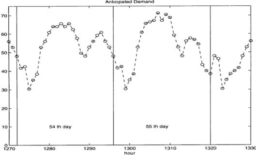
Demand is time-varying on an hourly basis, and demand on weekdays and week-ends is also different. However, it is periodic on a weekly basis, and the maximum demand usually occurs during weekdays. The characteristics of the anticipated de-mand used in this thesis is shown in Figure 3-1; each day is divided into twenty-four hours. During each hour, demand is constant. In this thesis, the maximum antici-pated demand is equal to 72.5 (power) units and the minimum anticiantici-pated demand is equal to 30.4 units.5

3.2.3

Bids

The generators submit their bids consisting of price and quantity (Pi[K],Xi[K]). Although the anticipated demand varies with time, the generator proposes just one price for a one-day schedule. The generators are obliged to set their offer prices

(P[K]) relating to their offer quantities (Xi[K]) by their marginal-cost functions.

Hence,

C,(X4 [K])

Pi[K] = OCi(X[K]) (3.4)

OXi[K]

4_{von der Fehr and Harbord [15] state (in footnote 2, p. 532) that "Green and Newbery also}

assume downward sloping demand curves, whereas completely inelastic demand would seem to be more appropriate for the UK industry."

5_{Note that the total assigned capacities always exceed the maximum anticipated demand or are}

X,[K] = P[K] -

(3.5)

2ai

Note that the offer quantity determines the maximum power that the generator will be willing to generate at that offer price or

Q < Xi[K] (3.6)

The P[K] is maximum when

Pimax[K] = C([K]) (3.7)

mXi [K]

Similarly, the generator actually offers a single step-supply function bid in which the maximum power supplied relates to the offer price by the generator's marginal-cost function. An example of the offer bid is shown in Figure 3-2. This figure shows that the generator submits the bid such that it will not operate more than the offer capacity (Xi[K]) at the offer price (Pi[K]).

3.2.4

The ISO

The ISO schedules the generators so that the anticipated demand is always met. The

ISO sets the market clearing price for each hour equal to the price proposed by the marginal operating generator in that hour. The generators are scheduled to operate in "the price merit order." In this model, the generator submits a single-step supply function bid; therefore, there is one price from each generator. The ISO arranges the offer prices of the generators in price-order. The generator offering the lowest price is scheduled to operate first. Thus the offer price of the generator with the highest price scheduled in each period, is announced as the market-clearing price. In addition, in some periods, the generators might offer the bids such that the demand might not be covered by the total offer quantities. The ISO will uniformly reschedule all generators' supply by using the Economic Dispatch (ED) technique so demand is met, and set the market clearing price in that period equal to the maximum price of

the offer prices and the prices calculated from ED.6

3.2.5

The Strategy

The market is formulated as one dynamic game. From a game theory perspective, the players participating in any game, play the game according to the previously specified strategies. A strategy for a player is a complete plan of action-it specifies a

feasible action for the player in every contingency in which the player might be called to act. In this bidding game, the generators adopt the given decision-making strategy

uniformly. Therefore, the generator will 'move' based on the same strategy.

3.2.6

Common Knowledge

Common knowledge is defined here as the information that is shared among the gen-erators. Similarly, the generators will have the same information, if the information is common knowledge. In this bidding game, common knowledge includes:

1. The anticipated demand for scheduling for the following day. 2. The previous and current market clearing price each hour.

However, as mentioned previously, the operating cost functions of individual genera-tors is not common knowledge. The amount of power purchased from each generator is also not public. Note that the maximum available capacity of each generator should be common knowledge, but it is not included here.7

6

See Appendix A for more detail about the ED. In fact, other criterion could be applied instead of the ED, if anticipated demand is not covered by the offer supply. For instance, it is possible to let the generators offer two price bids so that if demand is not met by the first price, there is room for the second-price market. But for simplicity, the ED solution is used. However, the ED will provide an optimal solution.

7_{The generators are assumed to have their "secret" long-term contracts (for the commited}

3.3

The Three-Generator Market Model

The dynamic model formulated in this thesis is the extended version of the static power market model. The static model which appears in previous research [13, 15] mainly consists of two generators or a duopoly. The static model assumes that op-erating cost functions of two generators are symmetric. In this thesis, however, one more generator is added and the operating cost functions of the generators are asym-metric. The additional generators in the model represent the general power markets more precisely because, in general, there are more than two generators participating in the market. In the real market, there are many generators with different technolo-gies. Hence, the model consisting of at least three generators with the asymmetric cost functions depicts the real market more accurately than a duopoly with the symmetric operating cost functions.

Because anticipated demand is inelastic and deterministic, price variations will have no effect on the customers' behavior. Therefore, the load has no significant role in this model. Moreover, there is no bidding process for the demand side. Thus demand has no dynamics.

As a result, in the simplified power market including the generators, the ISO and the load, only the generator section forms the dynamics of this market. Hence the 3-generator model is reduced to two sections: the generators and the ISO. In the generator section consisting the generators participating in the market, each generator determines its next bid based on the available information (i.e., common knowledge and the operating cost function). The ISO section performs the ISO's tasks which include equating supply and anticipated demand, and setting the market clearing price. The ISO announces the market clearing price in each period together with the anticipated demand of the next day. However the amount of power that each generator must produce is not public information so it is also not common knowledge.

3.3.1

The Generator Section

The generator section represents the generators' behavior. In this thesis, each gener-ator will offer only a single-step supply function bid. The genergener-ator's job is then to evaluate the next bid, such that the next day will yield the maximum profits. The generator determines its next bid by using all available information. The dynamic game is played by each generator individually, but it is assumed that each genera-tor has the same decision-making strategy. The bidding game is a finitely repeated game of complete but imperfect information; therefore, if there existed a unique Nash equilibrium in each bidding game, the generator would play the Nash equilibrium at every stage.

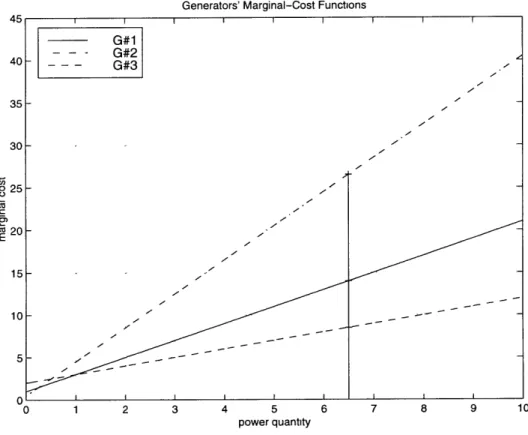
There are three generators with asymmetric operating cost functions in this model. The operating cost function of each generator is shown below :

Generator No. 1 C1(X) = X2 + X

Generator No. 2 C₂(X) = 2X2 + 0.5X Generator No. 3 C3(X) = 0.5X2 + 2X

The marginal cost function of each generator is: Generator No. 1 MC1(X) = 2X + 1

Generator No. 2 MC2(X) = 4X + 0.5

Generator No. 3 MC3(X) = X + 2

(Note that the operating cost function and the marginal-cost function are the func-tions of X instead of Q, because they refer to the functions that the generators use to formulate their bids.)

In this thesis, the marginal operating cost is an affine function of X, because the operating cost function of each generator is quadratic. The marginal cost function is derived by using the efficient pricing rule in which the marginal cost is set equal to the (given) market price [2]. The marginal-cost function of each generator is shown in Figure 3-3.

Definition 1 An expensive generator is a generator whose marginal cost is higher

ranges (i.e., X > 1). Similarly, that the most expensive generator's marginal-cost function lies above others' marginal-cost functions (along the (X) axis). (For instance,

from Figure 3-3, Generator No. 2 is the most expensive generator and Generator No. 3 is the cheapest generator.)

3.3.2

The ISO Section

The ISO section, on the other hand, represents the ISO's task, which is to equate the offer supply and the anticipated demand. Because the demand is inelastic, the ISO predicts the demand which has no relation to the variation in the market-clearing price. Hence, there are no dynamics in this section. The ISO is an operator who organises the power pool until the transaction is completed. The ISO arranges the offer step-supply functions provided by the generators in the price merit order (i.e., the lowest to the highest cost), schedules each generator until the anticipated demand is met and sets the market clearing price equal to the offer price by the marginal operating generator in each period. The market clearing prices become common knowledge as well as the anticipated next day demand. The special task for the ISO in this model, when the anticipated demand is not covered by the total offer supply, is to reschedule all generators' supply equally by using the solution calculated from the ED so the demand at that time is met.

3.4

Model Formulation

In order to formulate the bidding game, some specific definitions are key to under-standing the model set-up. Depending on the demand level, 24 hours can be divided into three periods: peak-load, mid-level and off-peak.8 Further assume that in off-peak periods at least one generator can supply the entire demand. On the other hand, during peak-load periods, all generators must activate their operations. Let us introduce: