HAL Id: hal-00317358
https://hal.archives-ouvertes.fr/hal-00317358
Submitted on 1 Jan 2002
HAL is a multi-disciplinary open access
archive for the deposit and dissemination of
sci-entific research documents, whether they are
pub-lished or not. The documents may come from
teaching and research institutions in France or
abroad, or from public or private research centers.
L’archive ouverte pluridisciplinaire HAL, est
destinée au dépôt et à la diffusion de documents
scientifiques de niveau recherche, publiés ou non,
émanant des établissements d’enseignement et de
recherche français ou étrangers, des laboratoires
publics ou privés.
bow shock
E. A. Lucek, T. S. Horbury, M. W. Dunlop, P. J. Cargill, S. J. Schwartz, A.
Balogh, P. Brown, C. Carr, K.-H. Fornacon, E. Georgescu
To cite this version:
E. A. Lucek, T. S. Horbury, M. W. Dunlop, P. J. Cargill, S. J. Schwartz, et al.. Cluster magnetic field
observations at a quasi-parallel bow shock. Annales Geophysicae, European Geosciences Union, 2002,
20 (11), pp.1699-1710. �hal-00317358�
Geophysicae
Cluster magnetic field observations at a quasi-parallel bow shock
E. A. Lucek1, T. S. Horbury1, M. W. Dunlop1, P. J. Cargill1, S. J. Schwartz2, A. Balogh1, P. Brown1, C. Carr1, K.-H. Fornacon3, and E. Georgescu4,5
1Space and Atmospheric Physics, The Blackett Laboratory, Imperial College, London, UK 2Astronomy Unit, Queen Mary, University of London, London, UK
3Institut f¨ur Geophysik und Meteorlogie, Technische Universit¨at Braunschweig, Germany 4Max-Planck-Institut f¨ur Extraterrestrische Physik, Garching, Germany
5Institut of Space Sciences, Bucharest, Romania
Received: 14 September 2001 – Revised: 24 June 2002 – Accepted: 17 July 2002
Abstract. We present four-point Cluster magnetic field data from a quasi-parallel shock crossing which allows us to probe the three-dimensional structure of this type of shock for the first time. We find that steepened ULF waves typically have a scale larger than the spacecraft separation (∼400–1000 km), while SLAMS-like magnetic field enhancements have differ-ent signatures in |B| at the four spacecraft, suggesting that they have a smaller scale size. In the latter case, however, the angular variations of B are similar, consistent with the space-craft making different trajectories through the same structure. The field enhancements have different orientations relative to a model bow shock normal, which might arise from different degrees of deceleration and deflection of the surrounding so-lar wind plasma. The observed rotation of the magnetic field rising from a direction approximately parallel to the model bow shock normal to a direction more perpendicular to the model normal across the field enhancement is consistent with previously published results. Successive magnetic field en-hancements or ULF waves, and the leading and trailing edges of the same structure, are found to have different orientations. Key words. Interplanetary physics (planetary bow shocks)
1 Introduction
The characteristics of collisionless planetary bow shocks are strongly dependent on the angle between the upstream mag-netic field and the bow shock normal, θBn. When θBn ex-ceeds 45◦, i.e. the shock normal is quasi-perpendicular to the upstream magnetic field, the shock tends to have a sharp tran-sition. Magnetic field observations typically show a short ramp in |B|, possibly with a “foot” ahead of the ramp, an overshoot after the ramp, or a high frequency wave train upstream of the ramp (e.g. Scudder et al., 1986). Quasi-perpendicular shocks have been studied in detail over many years and recently Cluster data have been used to examine
Correspondence to: E. A. Lucek ([email protected])
the structure of these shocks in three dimensions (Horbury et al., 2001, 2002).
When θBnis less than ∼45◦, particles are able to escape upstream, generating and interacting with a variety of waves situated in a foreshock region (e.g. Le and Russell, 1992a, b), and the shock transition is found to be far more extended and unsteady (e.g. Greenstadt et al., 1982). A combination of satellite observations (e.g. Gosling et al., 1989; Thomsen et al., 1990; Schwartz et al., 1992) and simulation work (e.g. Burgess, 1989; Thomas et al., 1990; Scholer, 1993) have led to a picture of a shock undergoing cyclic reformation, com-posed of a patchwork of magnetic field enhancements called SLAMS (Short, Large-Amplitude, Magnetic Structures) and regions between the SLAMS where the magnetic field is dis-turbed and the plasma is partially thermalised (e.g. Schwartz, 1991; Schwartz and Burgess, 1991; Scholer and Burgess, 1992; Giacalone et al., 1994).
SLAMS are identified as magnetic field signatures when the magnetic field magnitude is enhanced over the undis-turbed field by at least a factor of 2.5, with durations of the order of 10 s or so in the spacecraft frame. They have a rela-tively smooth profile and are, therefore, sometimes described as having a “near-monolithic” form. It has been suggested that they grow out of ULF waves in the foreshock region (Schwartz, 1991; Giacalone et al., 1993; Mann et al., 1994). They occur both in regions of ULF wave activity (isolated SLAMS) and within regions of stronger magnetic field pul-sations, associated with decelerated and heated plasma (em-bedded SLAMS). They are found to propagate sunward in the plasma frame, but are convected anti-sunward by the so-lar wind. They display mixed poso-larisation, biased towards right-hand polarised signatures (in the spacecraft frame), of-ten with the remnant of a left-handed (in the spacecraft frame), high frequency whistler wave on the leading edge, similar to that found at the lower amplitude, steepened ULF waves observed in the foreshock (Schwartz et al., 1992) com-monly called “shocklets”.
Statistical studies of SLAMS also show that the magnetic field rotates from a direction approximately parallel to a
model bow shock normal (upstream), to a direction closer to perpendicular, to a model bow shock normal (downstream), across the magnetic field enhancement (e.g. Mann et al., 1994). This magnetic field rotation changes the particle be-haviour at the SLAMS, since locally the magnetic field is similar to a quasi-perpendicular shock, which can lead to gy-rating ions downstream of the SLAMS, which scatter and partially thermalise the plasma. The study by Mann et al. (1994) of 18 isolated SLAMS also showed that the minimum variance direction, interpreted as the propagation direction, lay within 14.6 ± 8.7◦of a model bow shock normal.
Observational studies of the quasi-parallel bow shock have been complemented by simulations which have explored the behaviour of particles at structures within the shock transi-tion, and have shown that structures similar to SLAMS are generated (e.g. Scholer, 1993; Giacalone et al., 1994). A simulation of the foreshock region by Dubouloz and Scholer (1995) showed that SLAMS-like structures were generated when ULF waves, propagating against the solar wind flow, interacted with a high density, low energy diffuse ion popu-lation, as suggested by Giacalone et al. (1993) from a study of AMPTE data. Simulations have also shown that these structures typically evolve very quickly, on subsecond time scales. Giacalone et al. (1994) compared the results from a one-dimensional hybrid code to simulated multi-spacecraft observations through the same shock transition, and found that in this case spacecraft separated by only 188 km along the nominal shock normal direction saw significantly differ-ent signatures. Scale sizes of SLAMS-like structures occur-ring in simulations (e.g. Dubouloz and Scholer, 1995) have been found to be of the order of 15 ion inertial lengths per-pendicular to the shock normal, and a few tens of ion inertial lengths parallel to the shock normal. The simulation work described by Dubouloz and Scholer (1995) predicts that al-though SLAMS grow from the upstream ULF waves, which observationally have scale sizes of ∼1 RE (Le and Russell, 1990), SLAMS should have smaller scale sizes as differen-tial slowing of the incident flow was found to lead to frag-mentation of the ULF waves.
The structures within the quasi-parallel shock transition, therefore, are expected to be complex, possibly with dif-ferent scale lengths in difdif-ferent directions (Schwartz and Burgess, 1991; Dubouloz and Scholer, 1995), but single or dual spacecraft observations are not sufficient to probe their three-dimensional form. For the first time four-point ob-servations are available from the Cluster mission, launched in 2000 into a polar orbit, with an apogee of 19.6 RE and perigee of 4 RE. The choice of orbit means that bow shock crossings are biased to high latitude locations when apogee is near noon, although low latitude crossings do occur when apogee lies in the flanks of the magnetosphere.
The bow shock is one of the key regions for study us-ing Cluster data. Simultaneous observations by spacecraft pairs with different separation vectors relative to the plasma flow, expected bow shock normal, and magnetic field allow, in principal, the three-dimensional characteristics of struc-tures within the shock transition to be studied. We use the
observations with caution, however, since simulations (e.g. Giacalone et al., 1994) suggest that features within the shock evolve rapidly, on time scales of a few seconds or less, and might not be planar on scales of a few hundred to a thousand kilometres, which is approximately the scale of the Cluster tetrahedron during the observations made to date.
This study describes some of the characteristics of the magnetic field structures during the shock transition, and draws entirely on data from the four FGM instruments (Balogh et al., 2001). Although we concentrate on SLAMS, we also discuss the observational characteristics of upstream shocklets, which have a steepened leading edge (relative to their plasma frame propagation direction) and often also an associated whistler wave, for comparison with the SLAMS. A small number of intervals are discussed in detail, where we are able to estimate a propagation direction using both a method based on the relative timing of a feature at the four spacecraft, and minimum variance analysis. We also discuss minimum variance analysis of the upstream ULF wave field. SLAMS-like structures are distinguished from the magnetic signatures surrounding hot flow anomalies (HFA) (Schwartz, 1985, 1991) by their plasma signatures, and so here we can-not definitely identify SLAMS. We do, however, find mag-netic field structures with characteristics that are consistent with previous observations of SLAMS.
2 Analysis 2.1 Overview
In this paper we concentrate on one shock transition, on 2 February 2001 at ∼21:00 UT, when Cluster was at a lo-cal time of ∼15:00 LT. The upstream solar wind observed at ACE, approximately one hour earlier, had a velocity of
∼405 km/s, rising to ∼430 km/s at around 20:30 UT, imply-ing a jump in the solar wind velocity at the Earth at about 21:30 UT. The magnetic field magnitude at ACE was similar to that observed at times when Cluster was sampling undis-turbed solar wind plasma, ∼2.5 nT, and the number density at ACE was ∼2.8 cm−3. This implies an Alfv´en Mach number for the bow shock of ∼12–13 and a value for the ion inertial length in the undisturbed solar wind of ∼135 km. Figure 1 shows an overview of spin averaged magnetic field data (at 4 s resolution) recorded by Cluster 4. The shock transition, characterised by strongly compressive magnetic field varia-tions, lasts for several hours, and there are a number of bursts of smaller amplitude upstream wave activity, characteristic of the foreshock (e.g. just before 23:00 UT).
We order the magnetic field observations through the shock transition by comparing the instantaneous magnetic field direction with a bow shock normal derived from the Peredo et al. (1995) model under average solar wind con-ditions (see Horbury et al., 2002). In a study of 48 quasi-perpendicular bow shock crossings, Horbury et al. (2002) showed that there was good agreement, typically within
−90 0 °θ −180 0 180 φ ° −50 0 50 Bx −50 0 50 By −50 0 50 Bz 14:000 16:00 18:00 20:00 22:00 24:00 20 40 |B|
2 Feb. 2001, hour min (UT)
Fig. 1. Magnetic field data recorded by Cluster 4 through the
quasi-parallel shock on 2 February 2001. Data are displayed in the GSE coordinate system. Panels show magnetic field elevation (θ ) and longitude (φ) angles in degrees, three magnetic field components (Bx, By, Bz) and the magnetic field magnitude |B| in nT.
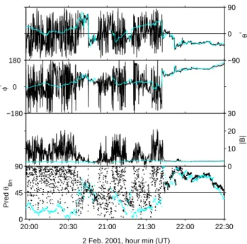
from the timing of the shock crossings at the four spacecraft. Using the simplifications outlined by Horbury et al. (2002), the model shock normal is likely to be accurate to within 10◦, which is sufficient to demonstrate the trends in the magnetic field direction across the shock on 2 February 2001. Fig-ure 2 shows the magnetic field data from Cluster 1 (in black) and ACE (in light blue) during the shock transition, together with the angle between the local magnetic field direction and the model bow shock normal (Pred θBn) estimated using the simplified Peredo model. Detailed comparison of the Cluster and ACE measurements shows that throughout the interval of interest, the delay time between ACE and Cluster is not constant, and that there are several intervals where the cor-respondence is poor. In Fig. 2 the time delay is altered such that the data sets show a good correspondence at three clear discontinuities (at ∼20:45, ∼21:40 and ∼21:50 UT). When the two data sets are dissimilar, such as between 20:50 and 21:10 UT, ACE data are not plotted.
Figure 2 shows that in the quiet magnetic field region up-stream of the shock transition (e.g. 21:45–22:30 UT), θBn rel-ative to the model shock normal is above 45◦, indicating that this region will be likely to give rise to a quasi-perpendicular shock. During intervals of good correspondence within the shock transition, the magnetic field direction measured at ACE is typically consistent with a quasi-parallel shock con-figuration. The local field at Cluster has been modified by the shock process, and within the compressive pulsation re-gions the values of θBn are more scattered, and tend to be biased towards 90◦. Such behaviour is expected from pre-vious studies which showed that across SLAMS structures,
−90 0 °θ −180 0 180 φ ° 0 10 20 30 |B| 20:00 20:30 21:00 21:30 22:00 22:30 0 45 90
2 Feb. 2001, hour min (UT)
Pred
θBn
Fig. 2. The angular variations of the spin-averaged magnetic field
at Cluster 1 (black) and upstream at ACE (light blue). Panels show magnetic field elevation (θ ) and longitude (φ) angles in GSE co-ordinates, magnetic field magnitude (|B|) in nT and the angle be-tween the model bow shock normal and the magnetic field (Pred
θBn). ACE data are lagged to give good correspondence between
the magnetic field angles seen at ACE and at Cluster. When the data sets do not have clear features in common, ACE data are not plotted, for example, between ∼20:50 and 21:10 UT.
the magnetic field tended to rotate from an orientation nearly parallel to the model bow shock normal, to a direction more perpendicular to the shock normal (e.g. Schwartz et al., 1992; Mann et al., 1994).
Figure 3 shows the Cluster orbit and spacecraft tetrahedron configuration on 2 February 2001. A cut though a nominal model bow shock is shown on each panel. At the end of the day, when the shock is encountered, Cluster 2 is separated from the other three spacecraft by about 1000 km in the X–
YGSEplane, mainly in the YGSEdirection, lying closer to the
nose of the magnetosphere. The other three spacecraft are quite closely aligned with the orbit in the X–YGSEplane,
al-though separated in ZGSE, with spacecraft separations of the
order of 400–800 km. Cluster 1 lies at the highest ZGSE, and
Cluster 2 and 3 lie further upstream than Cluster 4.
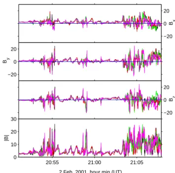
Figure 4 shows a section of the shock transition in more detail. This interval contains the clearest examples of SLAMS-like magnetic field enhancements, but unfortu-nately, there is poor correspondence between the ACE mag-netic field and the Cluster data during this time: two dis-continuities are observed at ACE (not shown), which would be expected to be seen in the Cluster data at approximately 20:50 UT and 21:03 UT, but neither are found to occur at Cluster.
Data from the four spacecraft are plotted, using the same colour scheme as for the orbit plot. It can be seen from
−5 0 5 10 15 −5 0 5 10 X GSE (RE) Z GSE (R E ) 20:00 UT 2 Feb. 2001, 00:00 − 24:00 UT −5 0 5 10 15 −5 0 5 10 X GSE (RE) Y GSE (R E ) 20:00 UT
Fig. 3. The Cluster orbit track and spacecraft configuration
pro-jected onto the X–ZGSE plane (top) and the X–YGSE plane
(bot-tom). The orbit is shown in a dotted line when the third component is negative. The asterisk indicates the start of the interval. Filled cir-cles indicate hourly markers along the orbit. The tetrahedron con-figuration is plotted on the orbit at around the time that the shock was encountered, expanded by a factor of 20 with the spacecraft in-dicated by black (Cluster 1), red (2), green (3) and magneta (4). A cut through a nominal bow shock location is shown on each panel for context.
this figure that the four spacecraft see similar features on large scales, but that there are significant differences at small scales, especially during the region of strong compressional activity after 21:03 UT. There is ultra-low frequency (ULF) wave activity from just after 20:55 UT, until 21:03 UT, which is interrupted by two large magnetic field magnitude
en-−20 0 20 Bx −20 0 20 B y −20 0 20 Bz 20:55 21:00 21:05 0 10 20 30 |B|
2 Feb. 2001, hour min (UT)
Fig. 4. Magnetic field data from the four spacecraft at 5 vectors/s
from a region of the shock transition. The spacecraft are indicated by black (Cluster 1), red (2), green (3) and magenta (4). Panels show the three magnetic field components (Bx, By, Bz) in GSE
coordinates, and the magnetic field magnitude (|B|), all in nT.
hancements. Earlier, between 20:53 and 20:55 UT, there is another burst of activity which also has some magnetic field enhancements embedded in it. There are smaller differences between the magnetic fields measured at the four spacecraft during the ULF wave activity than during the magnetic pul-sations, suggesting that the ULF waves are of larger scale, or evolving more slowly.
In the following sections we examine the correlation be-tween the four Cluster spacecraft at a number of magnetic field structures within and upstream of the shock transition. We first analyse two magnetic field enhancements, one of which is embedded in the region of compressive magnetic field pulsations between 20:53 and 20:55 UT, and is, there-fore, a candidate for an embedded SLAMS, and another which lies within the region of ULF wave activity, and is, therefore, a candidate for an isolated SLAMS. For com-parison with the magnetic field enhancements, we exam-ine examples of shocklets with associated upstream whistler waves. We also consider the characteristics of the ULF waves which occur in this interval, and lastly, we present a sharp transition into undisturbed solar wind.
2.2 Magnetic field structures within the shock transition 2.2.1 Interval 1: 20:54:30–20:55:30 UT
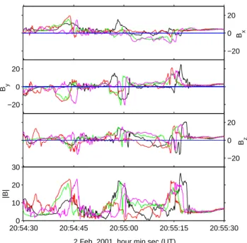
Figure 5 shows high resolution magnetic field data for two clear magnetic field magnitude enhancements which are em-bedded in further magnetic pulsations. The first is just be-fore 20:54:45 UT, and the second is at 20:55:15 UT. Between
−20 0 20 Bx −20 0 20 By −20 0 20 Bz 20:54:300 20:54:45 20:55:00 20:55:15 20:55:30 10 20 30 |B|
2 Feb. 2001, hour min sec (UT)
Fig. 5. Magnetic field data from the four spacecraft at 22 vectors/s
showing magnetic field magnitude enhancements within a pulsation region. The format of the figure is as in Fig. 4.
them is a structure less well correlated between the space-craft (at 20:55:00 UT). On these time scales, although the signatures at the four spacecraft are related, there are sig-nificant differences, suggesting that spatial changes occur on the order of the spacecraft separation, which at this time was between a few hundred and a thousand kilometres. Compar-ison of the ordering of the spacecraft shows that although the signatures appear to be convected towards the Earth (for ex-ample, the signature at Cluster 2 (red) or 3 (green) typically leads that at Cluster 4 (magenta)), the ordering of the space-craft varies both between the leading and trailing edges of the structures, and between the two structures, even though they are only separated by 30 s.
In the first case Cluster 1 (black) sees a much smaller en-hancement, despite Cluster 2 and Cluster 4 observing signa-tures of a similar magnitude before and after the enhance-ment at Cluster 1. This suggests that the difference between Cluster 2 or 4 and Cluster 1 arises from spatial variations of the structure rather than temporal evolution. The orbit plot (Fig. 3) shows that Cluster 1 lies at a significantly larger
ZGSEthan Cluster 2 or 4. Comparison with the second clear
example, at 20:55:15 UT, shows that in this case Cluster 1 sees a similar magnitude enhancement to the other three. Here, however, Cluster 2, 3 and 4 see a nearly simultaneous onset, while there is a delay before Cluster 1 sees the mag-netic field rise. This implies that the surface of the structure first encountered by the spacecraft lies parallel to the plane containing Cluster 2, 3 and 4. The spacecraft exit from the structure in a different order to the entry, suggesting that the orientations of the leading and trailing edges are different. It appears, therefore, that these structures are not planar on the
−90 0 °θ −180 0 180 φ ° 0 10 20 30 |B| 55:08 55:12 55:16 55:20 55:24 55:28 0 45 90 Pred θBn
2 Feb. 2001, hour 20 min sec (UT)
Fig. 6. The variation of the θBn angle predicted using the bow
shock model normal across the magnetic field enhancement at 20:55:15 UT. Panels show the magnetic field elevation (θ ) and lon-gitude (φ) angles in GSE coordinates, the magnetic field magnitude (|B|) and θBn.
scale of the tetrahedron. The timing differences between suc-cessive magnetic field enhancements might arise from differ-ent trajectories though the structures, or from the structures having different underlying orientations.
The second magnetic field enhancement, at 20:55:15 UT, is more similar between the four spacecraft. Figure 6 shows the change in the orientation of the magnetic field direction, relative to the model bow shock normal across this struc-ture. The angle between the two directions is denoted θBn. This figure shows that although there are differences between the magnetic field magnitude signatures at the four space-craft, the behaviour of the magnetic field direction at the four spacecraft is quite similar. Moving from right (upstream of the enhancement) to left (through the enhancement): up-stream of the leading edge, the magnetic field direction is within 45◦of the model bow shock normal; across the lead-ing edge θBnrises, with a slight plateau at the end of the sharp ramp, then rises more quickly to a value near 90◦within the enhancement. The magnetic field magnitude at Cluster 2 has a feature similar to a shock foot, typically observed at quasi-perpendicular shocks (e.g Scudder et al., 1986). Cluster 3 sees a similar feature, but it is less pronounced, and Clus-ter 4 and 1 observe short ramps, lasting for about 0.5 s, on the leading edge. This variation could be explained by rapid temporal evolution of the leading edge. The smaller system-atic variations in θBnjust ahead of the ramp, which are clear in the data from Cluster 1 and 4, are caused by low amplitude high frequency waves which are left-handed in the space-craft frame (with respect to the upstream magnetic field di-rection). This polarisation signature is consistent with
right-−500 0 500 −500 0 500 −500 0 500 GSE X (km) 2 Feb. 2001, 20:55 UT GSE Y (km) GSE Z (km)
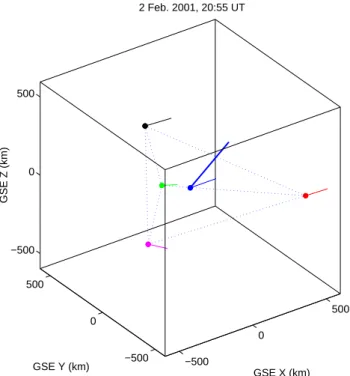
Fig. 7. A summary of the different estimates of the direction
nor-mal to the SLAMS surface: model nornor-mal (heavy blue line), timing derived normal (fine blue line), minimum variance directions esti-mated at the individual spacecraft (Cluster 1, 2, 3 and 4 represented by black, red, green and magenta, respectively)
handed whistler waves propatating sunward, but convected anti-sunward by the solar wind, hence reversing their polari-sation signature, and this is a well-known feature of shocklets (e.g. Omidi and Winske, 1990; Le and Russell, 1992b) and SLAMS (e.g. Schwartz et al., 1992).
Minimum variance analysis (MVA) can be used to find the minimum variance direction, which for a plane wave can be interpreted as the propagation direction. We have compared the results of MVA for each of the four spacecraft for the magnetic field enhancement at 20:55 UT, and have also es-timated a normal from the relative spacecraft timings of the ramp at the leading edge for comparison with MVA, using the method described by Schwartz (1998). When applying MVA to this event, we used intervals during which |B| was enhanced, excluding any intervals containing a whistler wave component, although it was found that the minimum variance directions were not strongly dependent on the data interval in this case. The normal from the discontinuity timing analysis is found to be n = (0.98, 0.14, -0.10) in GSE coordinates, which is at an angle of 25◦to the model bow shock normal,
nsh= (0.90, 0.34, 0.27).
The minimum variance directions for the four spacecraft are found to be e1 = (0.91, 0.13, -0.14); e2 = (0.94, 0.27,
-0.22); e3= (0.81, 0.39, -0.43); e4= (0.82, 0.23, -0.52). The
ratios between the intermediate and minimum eigenvalues for the MVA of data from each spacecraft exceed 4 in each case and are, therefore, well defined. The magnetic field en-hancement is observed to be right-handed at all four
space-craft. The angle between the minimum variance directions and the discontinuity timing normal is 2◦, 10◦, 26◦, 27◦, for Cluster 1, 2, 3 and 4, respectively. Each minimum variance direction lies at greater angles to the model normal than the timing normal: 27◦, 28◦, 42◦and 47◦, respectively.
The local magnetic field direction has been modified by the wave field, so it is useful to compare the propagation di-rection of the SLAMS structure, estimated either using tim-ing analysis or MVA, with the undisturbed magnetic field di-rection. It is not possible in this case to use the magnetic field observed by ACE for this purpose, because there is poor cor-respondence between the ACE and Cluster observations dur-ing this interval, as described in the Analysis section. There-fore, the propagation direction was compared with the quiet magnetic field direction recorded just before the wave activ-ity, although such a comparison is not ideal since the change in magnetic field character is likely to be associated with a change in underlying magnetic field direction. The propa-gation direction of the SLAMS structure was found to be at an angle of 50–75◦to the magnetic field direction in this re-gion. The SLAMS structure, therefore, appears to be more closely aligned with the model bow shock normal than with the underlying magnetic field direction.
The different estimates for the normal to the SLAMS structure are summarised in Fig. 7, which shows the Cluster tetrahedron at the time when the magnetic field enhancement was observed. The positions of the four spacecraft are indi-cated by the coloured dots, and the centre of the tetrahedron is indicated by the blue point. The thick blue line indicates the direction of the model normal, and the fine blue line in-dicates the normal estimated from timing analysis. The min-imum variance directions found for each individual space-craft are indicated by the lines at the positions of the differ-ent spacecraft. The agreemdiffer-ent between the minimum vari-ance direction and the discontinuity timing analysis normal is closest for Cluster 1, which is furthest out of the X–YGSE
plane. There is a systematic deflection of the minimum vari-ance direction away from the timing normal between Clus-ter 2, 3 and 4, which supports the hypothesis that the struc-ture is three-dimensional on the scale of the Cluster tetrahe-dron. Consequently, the timing derived normal is likely to give an average estimate of the normal over the tetrahedron scale. Comparison of the discontinuity timing normal with the bow shock model normal shows that they are separated by an angle of ∼25◦, with the discontinuity timing vector being deflected southward. Although the minimum variance directions show quite a lot of scatter, all are deflected south-ward relative to the bow shock model normal. The angle sep-arating the timing and model normals lies slightly outside the range found by Mann et al. (1994) of ∼15±9◦, and several of the angles between the minimum variance directions and the model normal lie substantially outside this range. Mann et al. (1994), however, only considered isolated SLAMS, while this structure is consistent with an embedded SLAMS, which is associated with deflected and decelerated plasma flow rel-ative to the undisturbed solar wind plasma, and such a deflec-tion is consistent with the sense of discrepancy in the normal
−20 0 20 Bx −20 0 20 B y −20 0 20 Bz 20:57:30 20:58:00 20:58:30 20:59:00 0 10 20 30 |B|
2 Feb. 2001, hour min sec (UT)
Fig. 8. Magnetic field data at 22 vectors/s in GSE coordinates, in
the same format at Fig. 5.
directions.
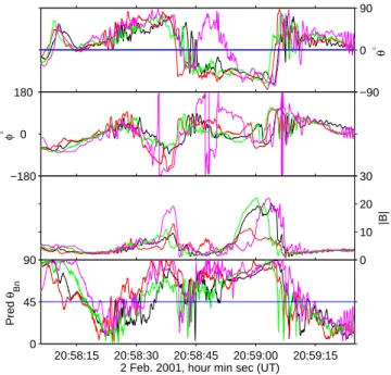
2.2.2 Interval 2: 20:57–21:00 UT
The second interval of magnetic field enhancements to be considered in detail occurs four minutes after the interval discussed in the previous section. Figure 8 shows the high resolution magnetic field data in the same format as Fig. 5. The magnetic field enhancements stand out clearly from the surrounding ULF wave activity. In this interval the mag-netic field enhancements are isolated from other strongly compressive magnetic field signatures, consistent with iso-lated SLAMS. The four spacecraft still see markedly differ-ent signatures. At the first structure (at 20:58:40 UT) Clus-ter 4, which lies earthward of ClusClus-ter 2 and 3, and further south than Cluster 1, observes a larger magnetic field magni-tude enhancement, despite the signature occurring at approx-imately the same time in all four spacecraft, suggesting that the signature does not arise from temporal variations. Clus-ter 2 and 4 each observe a distinct leading edge, while there is a less clear leading edge seen by Cluster 1 and 3.
At the second enhancement (at 20:59:00 UT), Cluster 4 observes a shorter enhancement than the other spacecraft, while Cluster 2 encounters a much smaller magnetic field magnitude than the other three. The variation in spacecraft ordering and observed signature is more likely to arise from spatial changes on scales of a few hundred to a thousand kilometres than temporal differences, since the structure nei-ther systematically grows nor decays at successive spacecraft crossings. Figure 3 shows that Cluster 2 lies approximately 1000 km from the other three spacecraft, separated almost parallel to the nominal shock surface. In this case then,
Clus-−90 0 °θ −180 0 180 φ ° 0 10 20 30 |B| 20:58:15 20:58:30 20:58:45 20:59:00 20:59:15 0 45 90 Pred θBn
2 Feb. 2001, hour min sec (UT)
Fig. 9. The variation of the θBnangle predicted using the bow shock
model normal across the two magnetic field enhancements during interval 2. Panels have the same format as in Fig. 6.
ter 2 might make a significantly different trajectory through the structure than the other three spacecraft, and the observed signature arises from spatial variations perpendicular to the nominal shock normal.
Figure 9 is in the same format as Fig. 6 and shows the mag-netic field direction, magmag-netic field magnitude, and the angle of the local magnetic field relative to a model bow shock nor-mal across the two magnetic field enhancements. Although Cluster 2 observes a smaller magnetic field magnitude at the second field enhancement (at ∼20:59 UT), the angular vari-ation through both structures is very similar to that seen by the other three spacecraft, which is in good agreement, es-pecially for the clearer of the two magnetic field enhance-ments. As in the previous example, the magnetic field up-stream makes an angle to the model bow shock normal of less than 45◦. Then, moving from right to left on Fig. 9, through the region with a high frequency wave (between ∼20:59:05 and 20:59:20 UT) and across the leading edge, the magnetic field rotates until this angle becomes nearly 90◦. The mag-netic field retains this direction through the region where |B| is high. The angular variations in the region between the two magnetic field enhancements are much more irregular, sug-gesting that processes are occurring on smaller scales during that interval. During the smaller magnetic field enhancement, however, the local magnetic field once again rotates to make an angle of nearly 90◦to the model bow shock normal. The similarity of the angular signatures seen by Cluster 2 to those seen by the other spacecraft shows that the shape of the struc-ture, measured by the magnetic field direction, is preserved over the separation distance to Cluster 2, despite the differ-ence in magnetic field magnitude.
−500 0 500 −500 0 500 −500 0 500 GSE X (km) 2 Feb. 2001, 20:59 UT GSE Y (km) GSE Z (km)
Fig. 10. Summary of the different estimates of the normal to the
SLAMS at 20:59 UT, in the same format as Fig. 7.
Since the |B| signature at Cluster 2 is significantly differ-ent from that at Cluster 1, 3 and 4, discontinuity timing anal-ysis cannot be applied to the |B| profile. Using the similar-ity of the angular variations, however, discontinusimilar-ity timing analysis (not shown) was applied to the θ signature, giving a normal direction which agreed with the model normal within 13◦and with the minimum variance directions from the four spacecraft within 20◦. The different estimates for the direc-tion normal to the SLAMS are shown in Fig. 10, using the same format as in Fig. 7. In this case minimum variance analysis applied to the data from the four spacecraft gives minimum variance directions which agree with the model normal within 10◦. This is consistent with the results found for isolated SLAMS by Mann et al. (1994). The better agree-ment between the calculated normal and minimum variance directions and the model normal might arise from the iso-lated nature of the enhancements which, if isoiso-lated SLAMS, are less likely to be associated with significant deceleration and deflection of the solar wind flow. A better agreement, therefore, would be expected between the orientation of the structure and the model bow shock normal.
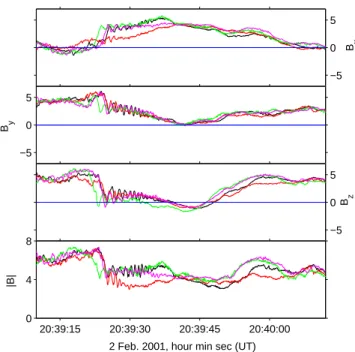
Once again the different estimates of the SLAMS propaga-tion direcpropaga-tion were compared with the magnetic field direc-tion just before this interval, and again the angular separadirec-tion of these vectors was found to be large: in the range 60–75◦, suggesting that the SLAMS was more closely aligned with the model bow shock normal than the background magnetic field direction. −5 0 5 Bx −5 0 5 By −5 0 5 B z 20:39:15 20:39:30 20:39:45 20:40:00 0 4 8 |B|
2 Feb. 2001, hour min sec (UT)
Fig. 11. Magnetic field data at 22 vectors/s in GSE coordinates,
in the same format at Fig. 5. The data show a shocklet with an upstream whistler wave.
2.3 Upstream shocklet characteristics
Figure 11 shows an example of a steepened upstream ULF wave, called a shocklet, at ∼20:39:17 UT. In this case Clus-ter 3 observes the shocklet first, when it has a slightly shal-lower gradient and a less well developed high frequency wave than later, when it is encountered by the other three spacecraft, who all observe a steeper leading edge (right-hand side) and a better developed high frequency wave train. The delay between the observations at Cluster 3 and at the other three spacecraft is only about 1 s. Since the signature is simultaneous at Cluster 1, 2 and 4, this suggests that the normal to the structure lies nearly perpendicular to the plane containing the three spacecraft. Applying timing disconti-nuity analysis to the leading edge gives a normal of 0.75, 0.66–0.02, which is within 10◦of the normal to this plane. The timing analysis normal is within 30◦of the model bow shock normal, a slightly greater angle than observed for ei-ther of the SLAMS events. Such an observation is consistent with the simulation of Dubouloz and Scholer (1995), which showed that as ULF waves approached the shock, and devel-oped into SLAMS-like structures, they become more closely aligned with the shock.
The appearance of the shocklet at Cluster 1, 2 and 4 is very similar, although there are small changes in the frequency of the upstream whistler wave. Therefore, although the differ-ence in the signatures at Cluster 3 and the other spacecraft might be spatial in nature, it seems more likely to reflect a temporal evolution on short time scales. The two consecu-tive structures in Fig. 11 (the shocklet at ∼20:39:17 UT and the ULF wave just before 20:39:40 UT) show different
space-tures have different orientations. Minimum variance analysis of the shocklet signature measured by Cluster 2 shows that the ratio between the intermediate and minimum eigenratios is less than 2, indicating that the minimum variance tion is ill defined in this case. The minimum variance direc-tions calculated for the signature observed by the other three spacecraft differ by 15–20◦but differ from the timing derived estimate for the normal by up to 30◦. The discrepancy might arise because the shocklet has only a small variation in mag-netic field direction, and hence, the contribution of higher frequency changes increases. This is consistent with the ra-tio of intermediate to minimum eigenvalues exceeding 2, but the observed absence of a clear rotation on a hodogram.
Comparison of the timing derived normal with the back-ground magnetic field direction, estimated from ACE data with an appropriate delay, shows that these directions differ by 53◦. The delay is calculated using the correspondence be-tween a clear discontinuity observed at Cluster at ∼20:45 UT, having been observed at ACE 4167s earlier. Using an esti-mate of the background magnetic field from Cluster during a minute of quiet data immediately following the wave activity, gives a separation of the normal from the background mag-netic field of approximately 65◦. The three minimum vari-ance directions lie closer to the background magnetic field estimated from the ACE observations, falling in the range of 30–40◦. Each estimate of the propagation direction, however, for this example, lies closer to the model bow shock normal than to the background magnetic field vector.
Figure 12 shows a second example of a shocklet, observed about two hours later at ∼22:44 UT, which appears to be sta-ble during the time in which the tetrahedron traverses the structure. This structure is found within ULF wave activ-ity, just before a very sharp transition into undisturbed solar wind a few minutes later, which is discussed in the next sec-tion. Each of the Cluster spacecraft observe a well developed high frequency wave just upstream of the leading edge, al-though the frequencies of the waves differ slightly between spacecraft. The high frequency waves are again left-hand po-larised, consistent with a whistler wave being convected anti-sunward by the solar wind flow. This example also demon-strates that the orientations of the leading and trailing edges are different. This can be seen from the spacecraft ordering through the signature. The leading edge (right-hand side) is observed first by Cluster 2, and then almost simultane-ously by Cluster 1, 3 and 4. The trailing edge (left-hand side) was observed first by Cluster 2, but the ordering of the other three spacecraft is different. Using discontinuity timing anal-ysis gives leading and trailing edge normal directions which are ∼21◦ apart. The polarisation of the shocklet signature observed by each spacecraft, excluding the high frequency waves, is right-handed, and there is good agreement between the minimum variance direction and the normal calculated for the leading edge (within ∼5 and 10◦). That this shocklet shows greater consistency between the minimum variance di-rections found for each spacecraft and the timing derived nor-mal might arise from the larger amplitude magnetic field
ro-−5 0 5 Bx −5 0 5 By −5 0 5 Bz 22:43:30 22:44:00 22:44:30 22:45:00 0 5 10 |B|
2 Feb. 2001, hour min sec (UT)
Fig. 12. Magnetic field data at 22 vectors/s in GSE coordinates, in
the same format at Fig. 5. The data show a shocklet at 22:44 UT, with an upstream whistler wave.
tation across the wave. The leading edge and minimum vari-ance derived normals lay within 20–30◦of the background magnetic field, estimated using ACE data with an appropri-ate delay, which is marginally more closely aligned with the background magnetic field than that found for either the pre-vious shocklet examples or either of the SLAMS. Although the location of the satellites far upstream of the expected bow shock position means that the model bow shock nor-mal direction is less relevant, the angle between the leading edge normal and the model bow shock normal was calculated for comparison with the analysis applied to the SLAMS and previous shocklet. The different estimates of the previous shocklet propagation direction lay within ∼35◦of the model bow shock normal. A greater angle between the propagation direction estimates and the model shock normal is consistent with the waves further upstream being less influenced by the presence of the shock.
2.4 Upstream ULF wave characteristics
In the previous three subsections the characteristics of a small number of magnetic field signatures have been described in detail. For these cases the four satellites observed similar sig-natures, allowing an estimate to the made of their orientation and motion. Comparison with minimum variance analysis, interpreting the minimum variance direction as the propaga-tion direcpropaga-tion that has been used in the past for single space-craft observations, shows significant differences between the methods. These might arise from the deviations of the struc-tures from planarity on the tetrahedron scales, or from inher-ent uncertainties in the minimum variance technique, espe-cially for events with small angular changes (Eastwood et al.,
−6 0 6 Bx −6 0 6 By −6 0 6 Bz 22:46 22:47 22:48 22:49 0 5 10 |B|
2 Feb. 2001, hour min (UT)
Fig. 13. Magnetic field data at 22 vectors/s in GSE coordinates, in
the same format at Fig. 5. The data show an abrupt transition from a region populated by ULF waves and shocklets, to undisturbed solar wind.
2002).
The correlation between the different spacecraft is typi-cally greater during ULF wave activity than is observed for the SLAMS-like signatures, suggesting that the ULF wave scale is larger than that of the magnetic field enhancements, and significantly larger than the spacecraft tetrahedron. This is consistent with the simulations of Dubouloz and Scholer (1995), which showed that differential slowing of the plasma ahead of the shock fragmented the structures that were ob-served to grow out of the ULF wave field, leading to a smaller scale size. Successive ULF waves, however, typically show different spacecraft ordering, indicating that they do not have the same orientation. Frequently, as can be seen in Figs. 8, 11 and 12, a single ULF wave will also show different space-craft ordering at the leading and trailing edges, suggesting that the leading and trailing edges can also have different orientations. The smooth, but irregular profile of the ULF waves makes spacecraft timing estimates of their orientation difficult to measure. In addition, minimum variance analysis of the ULF wave field in this case gives minimum variance directions that show a large scatter, both between the differ-ent spacecraft observations of any particular wave, and also between successive ULF waves. The scatter varies between waves, but can be large, of the order of 45–90◦. This scat-ter makes it difficult to compare the characscat-teristics of ULF waves and SLAMS-like structures. The ULF waves observed at this shock, however, do not show regular angular varia-tions, and the comparison of the two types of structure would be better compared using an interval when the ULF waves are regular with larger amplitude angular variations, with well-defined and consistent minimum variance directions and a
form where timing analysis can be applied. 2.5 Transition into undisturbed solar wind
Figure 13 shows a transition from the region containing upstream ULF waves and shocklets, into undisturbed solar wind. It is remarkable for the abrupt nature of the transi-tion, which lasts only for ∼1.5 s. The timing analysis nor-mal is found to differ significantly (by ∼60◦), mainly in the
Y–ZGSE direction, from the model bow shock normal,
sug-gesting that, in this case, the orientation of the boundary is not controlled by the bow shock orientation. This signa-ture might be caused by a solar wind discontinuity propa-gating past the tetrahedron, and we note that it appears to be extremely abrupt. Later transitions are not found to be as sharp and perhaps reflect the spacecraft moving from mag-netic field lines which are connected with the shock, to those which are not.
3 Discussion and conclusions
We have described some of the features observed at a quasi-parallel shock observed by Cluster on 2 February 2001. We described the structure of magnetic field enhancements that have signatures consistent with that expected for SLAMS, and steepened upstream ULF waves (shocklets). We also dis-cussed briefly the characteristics of the ULF waves.
Although the spacecraft observe broadly similar struc-tures, significant variations between the signatures at the dif-ferent spacecraft are also found. A distinct difference is found between the scale of the upstream ULF waves and shocklets, and the magnetic field enhancements and pulsa-tion regions within the shock transipulsa-tion. The upstream ULF waves appear to be of significantly greater scale, apparently much greater than the tetrahedron scale of 400–1000 km, which is consistent with the expected scales from previous work of ∼1 RE. The scale of the SLAMS-like magnetic field enhancements appears to be shorter than the 0.5–1 RE scales found for the upstream ULF wave field (Schwartz, 1991) since significant differences occur between spacecraft. This is consistent with the evolution of SLAMS from the ULF wave field observed in the simulations described by Dubouloz and Scholer (1995), and their subsequent frag-mentation by wave front refraction close to the shock. Both shocklets and magnetic field enhancements, however, show varying orientations between successive events, and fre-quently between the leading and trailing edges of the same event. These results suggest that the structures are not typ-ically planar on the current spacecraft separation scales of a few hundred to a thousand kilometres, which is smaller than the SLAMS scale size of 15–30 ion inertial lengths found by Dubouloz and Scholer (1995).
It is possible that the spacecraft differences observed through the SLAMS arises from the spacecraft sampling sig-nificant curvature on the scale of the tetrahedron, and that the orientations of the SLAMS might be ordered on a global
shock as a patchwork of three-dimensional structures first suggested by Schwartz and Burgess (1991). We note, how-ever, that although the shocklets and ULF waves appear to be of larger scale than the SLAMS, they still appear to have a va-riety of orientations. If SLAMS do develop from ULF waves, then a variety of orientations might be retained. We also ex-amined the data for signatures consistent with the growth of SLAMS-like structures. Although we have not found clear evidence of such time evolution, it is possible that it is hid-den by the spatial variations between the satellites.
In a number of SLAMS-like magnetic field enhancements we find that the angular variation of the magnetic field is better correlated between spacecraft than the magnetic field magnitude, and we find that the θBn value, calculated from the local magnetic field and a model bow shock normal, rises to quasi-perpendicular values within magnetic field enhance-ments at all spacecraft, as expected from previous observa-tions (Mann et al., 1994), despite differences in the profile of |B|. Nevertheless, any combination of the spacecraft data which assumes that the structure is planar, for example, dis-continuity timing analysis, must still be applied with caution, since curvature of the structure will bias the results. In ad-dition, the discontinuity timing method is sensitive to small differences in the relative times, making it difficult to apply with confidence unless the four spacecraft observe near iden-tical signatures.
The results of the timing and minimum variance analy-sis we have presented here suggest that two magnetic field enhancements, both of which have magnetic signatures con-sistent with SLAMS, have different orientations relative to the model bow shock normal. Clearly a greater number of magnetic field enhancements must be studied before general conclusions can be drawn about SLAMS properties, but we propose that the larger deviation between the estimated prop-agation direction and the model bow shock normal of the first example might arise from it being embedded in decelerated and deflected solar wind, while the other, which is closely aligned with the model bow shock normal, lies in relatively undisturbed plasma.
Analysis of two examples of upstream shocklets showed that the one located further upstream was less well aligned with the model bow shock normal, consistent with the plasma being less influenced by the shock in this region. Compari-son between the orientations of shocklets and SLAMS with respect to the background magnetic field was hampered by a poor estimate of the background field in the region con-taining the SLAMS-like features, but the results suggested that shocklets might be more closely aligned with the back-ground magnetic field than the SLAMS, consistent with the simulation results of Dubouloz and Scholer (1995). The ULF waves observed on this day showed different orientations at their leading and trailing edges, but had a smooth profile with only small angular variations, and showed variations between spacecraft, making these ULF waves poor candidates for dis-continuity timing analysis.
We have demonstrated the potential of Cluster
observa-structures. A statistical study of the scales and orientations of SLAMS, shocklets and ULF waves with respect to the shock and the magnetic field requires the analysis of multiple events, under conditions when good estimates of these quan-tities can be made. In addition, multiple observations are re-quired, at a range of tetrahedron scales, in order to examine any dependence of the scale size on direction, such as sys-tematic differences in the scale size along the two directions perpendicular to the nominal shock normal. The future sepa-ration strategy for Cluster will lead to quasi-parallel shock observations being made with a tetrahedron of spacecraft separated by only ∼100 km. Better correlation should be observed between the different spacecraft under these con-ditions, allowing for the propagation directions and orienta-tions of the enhancements to be measured more accurately. Later in the mission, larger tetrahedron scales are planned (∼REscales), which will allow for a better estimation of the scale size of the magnetic field enhancements to be made. We might expect a rapid fall off in the inter-spacecraft cor-relation if the enhancements are only a little larger than the current tetrahedron, but if the structures are large, with sig-nificant spatial evolution across them, a more gradual fall in the correlation as the distance is increased is likely.
The upstream solar wind velocity observed by ACE pro-vides a useful context for this shock, but local plasma mea-surements from the CIS instrument will be more relevant, al-lowing us to estimate the plasma frame propagation velocity and to relate the spacecraft separation vectors to the plasma flow direction. A more definitive identification of SLAMS would also be possible. One key question which remains to be answered is the effect which SLAMS have on the plasma, and future collaborative work is planned in order to address this topic.
Acknowledgements. Analysis of Cluster data at Imperial College is
supported by PPARC. T. Horbury is supported by a PPARC Fellow-ship. We gratefully acknowledge the NASA/GSFC CDAWeb for access to the ACE MFI solar wind magnetic field data (provided by N. Ness, Bartol Research Institute) and SWE electron density data (provided by D. J. MacComas, Los Alamos National Laboratory).
Topical Editor G. Chanteur thanks M. Goldstein, A. Mageney and another Referee for their help in evaluating this paper.
References
Balogh, A., Carr, C. M., Acu˜na, M. H., Dunlop, M. W., Beek, T. J., Brown, P., Fornacon, K.-H., Georgescu, E., Glassmeier, K.-H., Harris, J., Musmann, G., Oddy, T., and Schwingenschuh, K.: The Cluster Magnetic Field Investigation: overview of in-flight per-formance and initial results, Ann. Geophysicae, 19, 1207–1217, 2001.
Burgess, D.: Cyclic behaviour at quasi-parallel collisionless shocks, Geophys. Res. Lett., 16, 345–348, 1989.
Dubouloz, N. and Scholer, M.: Two-dimensional simulations of magnetic pulsations upstream of the Earth’s bow shock, J. Geo-phys. Res., 100, 9461–9474, 1995.
Eastwood, J. P., Balogh, A., Dunlop, M. W., Horbury, T. S., and Dandouras, I.: Cluster observations of fast magnetosonic waves in the terrestrial foreshock, submitted to Geophys. Res. Lett., 2002.
Giacalone, J., Schwartz, S. J., and Burgess, D.: Observations of suprathermal ions in association with SLAMS, Geophys. Res. Lett., 20, 149–152, 1993.
Giacalone, J., Schwartz, S. J., and Burgess, D.: Artificial spacecraft in hybrid simulations of the quasi-parallel Earth’s bow shock: analysis of time series versus spatial profiles and a separation strategy for Cluster, Ann. Geophysicae, 12, 591–601, 1994. Gosling, J. T., Thomsen, M. F., Bame, S. J., and Russell, C. T.: Ion
reflection and downstream thermalization at the quasi-parallel bow shock, J. Geophys. Res., 94, 10 027–10 037, 1989. Greenstadt, E. W., Hoppe, M. M., and Russell, C. T.:
Large-amplitude magnetic variations in quasi-parallel shocks: corre-lation lengths measured by ISEE 1 and 2, Geophys. Res. Lett., 9, 781–784, 1982.
Horbury, T. S., Cargill, P. J., Lucek, E. A., Balogh, A., Dunlop, M. W., Oddy, T. M., Carr, C., Brown, P., Szabo A., and Fornacon, K.-H.: Cluster magnetic field observations of the bowshock: ori-entation, motion and structure, Ann. Geophys., 19, 1399–1409, 2001.
Horbury, T. S., Cargill, P. J., Lucek, E. A., Eastwood, J., Balogh, A., Dunlop, M. W., Fornacon, K.-H., and Georgescu, E.: Four spacecraft measurements of the quasi-perpendicular terrestrial bowshock: orientation and motion, J. Geophys. Res., doi.: 10.1029/201JA000273, 107, 2002.
Le, G. and Russell, C. T.: A study of the coherence length of ULF waves in the Earth’s foreshock, J. Geophys. Res., 95, 10 703– 10 706, 1990.
Le, G. and Russell, C. T.: A study of ULF wave foreshock mor-phology – I: ULF foreshock boundary, Planet. Space Sci., 40, 1203–1213, 1992a.
Le, G. and Russell, C. T.: A study of ULF wave foreshock morphol-ogy – II: Spatial variation of ULF waves, Planet. Space Sci., 40, 1215–1225, 1992b.
Mann, G., L¨uhr, H., and Baumjohann, W.: Statistical analysis of short large-amplitude magnetic field structures in the vicinity of the quasi-parallel bow shock, J. Geophys. Res., 99, 13 315– 13 323, 1994.
Omidi, N. and Winske, D.: Steepening of kinetic magnetosonic waves into shocklets: simulations and consequences for plane-tary shocks and comets, J. Geophys. Res., 95, 2281–2300, 1990. Peredo, M., Slavin, J. A., Mazur, E., and Curtis, S. A.: Three-dimensional position and shape of the bow shock and their vari-ation with Alfv´enic, sonic and magnetosonic Mach numbers and interplanetary field orientation, J. Geophys. Res., 100, 7908– 7916, 1995.
Scholer, M.: Upstream waves, shocklets, short large-amplitude magnetic structures and the cyclic behaviour of oblique quasi-parallel collisionless shocks, J. Geophys. Res., 98, 47–57, 1993. Scholer, M. and Burgess, D.: The role of upstream waves in su-percritical quasi-parallel collisionless shock reformation, J. Geo-phys. Res., 97, 8319–8326, 1992.
Schwartz, S. J.: An active current sheet in the solar wind, Nature, 318, 269–271, 1985
Schwartz, S. J.: Magnetic field structures and related phenomena at quasi-parallel shocks, Adv. Space Res., 11, 9231–9240, 1991. Schwartz, S. J.: Shock and discontinuity normals, Mach
num-ber, and related parameters, in: Analysis methods for multi-spacecraft data, (Eds) Paschmann, G. and Daly, P. W., ESA Pub-lications Division, Noordwijk, The Netherlands, 1998.
Schwartz, S. J. and Burgess, D.: Quasi-parallel shocks: a patchwork of three-dimensional structures, Geophys. Res. Lett, 18, 373– 376, 1991.
Schwartz, S. J., Burgess, D., Wilkinson, W. P., Kessel, R. L., Dun-lop, M., and L¨uhr, H.: Observations of short large-amplitude magnetic structures at a quasi-parallel shock, J. Geophys. Res., 97, 4209–4227, 1992.
Scudder, J. D., Mangeney, A., Lacombe, C., Harvey, C. C., Aggson, T. L., Anderson, R. R., Gosling, J. T., Paschmann, G., and Rus-sell, C. T.: The resolved layer of a collisionless, high β, supercrit-ical, quasi-perpendicular shock wave 1. Rankine-Hugoniot ge-ometry, currents, and stationarity, J. Geophys. Res., 91, 11 019– 11 052, 1986.
Thomas, V. A., Winske, D., and Omidi, N.: Re-forming supercrit-ical quasi-parallel shocks 1. One- and two-dimensional simula-tions, J. Geophys. Res., 95, 18 809–18 819, 1990.
Thomsen, M. F., Gosling, J. T., Bame, S. J., and Russell, C. T.: Magnetic pulsations at the quasi-parallel shock, J. Geophys. Res., 95, 957–966, 1990.