Domain Decomposition Preconditioners for
Higher-Order Discontinuous Galerkin Discretizations
by
Laslo Tibor Diosady
S.M., Massachusetts Institute of Technology (2007)
B.A.Sc., University of Toronto (2005)
Submitted to the Department of Aeronautics and Astronautics
ACHIES
in partial fulfillment of the requirements for the degree ofA CHE
S
Doctor of Philosophy
Yat the
APR
2
MASSACHUSETTS INSTITUTE OF TECHNOLOGY
September 2011
@
Massachusetts Institute of Technology 2011. All rights reserved.
Author...
o A
a
s-ona-es
Department of Aeronautics and Astron201s
C(1-1 A-r-,\ Sept 2A2011
C ertified by ...
C ertified by ...
C ertified by ...
A ccepted by ...
David
Darmofal
Professor of Aeronautics and Astronautics
/,*
ThefisSupervisor
...
Alan Edelman
Pr es or of Mathematics
i~ t =----is Committee
.
...
Jaime Peraire
Professorbf Aeronautics and Astronautics
Thesis Committee
Eytan H. Modiano
Professor of Aeronautics and Astronautics
Chair, Committee on Graduate Students
Domain Decomposition Preconditioners for
Higher-Order Discontinuous Galerkin Discretizations
by
Laslo Tibor Diosady
Submitted to the Department of Aeronautics and Astronautics on Sept 23, 2011, in partial fulfillment of the
requirements for the degree of Doctor of Philosophy
Abstract
Aerodynamic flows involve features with a wide range of spatial and temporal scales which need to be resolved in order to accurately predict desired engineering quantities. While computational fluid dynamics (CFD) has advanced considerably in the past 30 years, the desire to perform more complex, higher-fidelity simulations remains. Present day CFD simu-lations are limited by the lack of an efficient high-fidelity solver able to take advantage of the massively parallel architectures of modern day supercomputers. A higher-order hybridizable discontinuous Galerkin (HDG) discretization combined with an implicit solution method is proposed as a means to attain engineering accuracy at lower computational cost. Domain decomposition methods are studied for the parallel solution of the linear system arising at each iteration of the implicit scheme.
A minimum overlapping additive Schwarz (ASM) preconditioner and a Balancing Do-main Decomposition by Constraints (BDDC) preconditioner are developed for the HDG discretization. An algebraic coarse space for the ASM preconditioner is developed based on the solution of local harmonic problems. The BDDC preconditioner is proven to converge at a rate independent of the number of subdomains and only weakly dependent on the solution order or the number of elements per subdomain for a second-order elliptic problem. The BDDC preconditioner is extended to the solution of convection-dominated problems using a Robin-Robin interface condition.
An inexact BDDC preconditioner is developed based on incomplete factorizations and a p-multigrid type coarse grid correction. It is shown that the incomplete factorization of the singular linear systems corresponding to local Neumann problems results in a non-singular preconditioner. The inexact BDDC preconditioner converges in a similar number of iterations as the exact BDDC method, with significantly reduced CPU time.
The domain decomposition preconditioners are extended to solve the Euler and Navier-Stokes systems of equations. An analysis is performed to determine the effect of boundary conditions on the convergence of domain decomposition methods. Optimized Robin-Robin interface conditions are derived for the BDDC preconditioner which significantly improve the performance relative to the standard Robin-Robin interface conditions. Both ASM and BDDC preconditioners are applied to solve several fundamental aerodynamic flows. Numerical results demonstrate that for high-Reynolds number flows, solved on anisotropic meshes, a coarse space is necessary in order to obtain good performance on more than 100 processors.
Thesis Supervisor: David L. Darmofal
Acknowledgments
I would like to thank all of those who helped make this work possible. First, I would like to thank my advisor Prof. David Darmofal, for giving me the opportunity to work with him. I am grateful for his guidance and encouragement throughout my studies at MIT. Second, I would like to thank my committee members Profs. Alan Edelman and Jaime Peraire for their criticism and direction throughout my PhD work. I would also like to thank my thesis readers Prof. Qiqi Wang and Dr. Venkat Venkatakrishnan for providing comments and
suggestions on improving this thesis.
This work would not have been possible without the contributions of the ProjectX team past and present (Julie Andren, Garrett Barter, Krzysztof Fidkowski, Bob Haimes, Josh Krakos, Eric Liu, JM Modisette, Todd Oliver, Mike Park, Huafei Sun, Masa Yano). Partic-ularly, I would like to acknowledge JM whose been a good friend and office mate my entire time at MIT.
I would like to thank my wife, Laura, my parents, Klara and Levente, and my brother, Andrew, for their encouragement throughout my time at MIT. Without their love and sup-port this work would never have been completed.
Finally, I would like to acknowledge the financial support I have received throughout my graduate studied. This work was supported by funding from MIT through the Zakhartchenko Fellowship and from The Boeing Company under technical monitor Dr. Mori Mani. This research was also supported in part by the National Science Foundation through TeraGrid
Contents
1 Introduction 1.1 Motivation . . . . 1.2 Background . . . . 1.2.1 Higher-order Discontinu 1.2.2 Scalable Implicit CFD 1.2.3 1.2.4 1.2.5 1.3 Thesis 1.3.1 1.3.2 Domain Decomposition Large Scale CFD simul Balancing Domain Dec Overview . . . . Objectives . . . . Thesis Contributions .. . . . . . . .
ous Galerkin Methods . . . . Thr... Theory . . . . ations . . . . )mposition by Constraints . . . . . . . . . . . . . .
2 Discretization and Governing Equations
2.1 HDG Discretization . . . . 2.2 Compressible Navier-Stokes Equations . . . . 2.3 Boundary Conditions . . . . 2.4 Solution M ethod . . . . 3 Domain Decomposition and the Additive Schwarz Method 3.1 Domain Decomposition . . . . 3.2 Additive Schwarz method . . . . 3.3 Numerical Results . . . . 4 Balancing Domain Decomposition by Constraints
4.1 A Schur Complement Problem . . . . 4.2 The BDDC Preconditioner . . . . 4.3 The BDDC Preconditioner Revisited . . . . 4.4 Convergence Analysis . . . . 4.5 Robin-Robin Interface Condition . . . . 4.6 Numerical Results . . . . 5 Inexact BDDC
5.1 A Note on the BDDC Implementation . . . . 5.2 BDDC using Incomplete Factorizations . . . . 5.2.1 Inexact Harmonic Extensions . . . . 5.2.2 Inexact Partially Assembled Solve . . . .
5.2.3 One or Two matrix method . . . . 81
5.3 Inexact BDDC with p-multigrid correction . . . . 82
5.3.1 Inexact Harmonic Extensions . . . . 82
5.3.2 Inexact Partially Assembled Solve . . . . 83
5.4 Numerical Results . . . . 84
5.4.1 Inexact BDDC using Incomplete Factorizations . . . . 85
5.4.2 Inexact BDDC with p-multigrid correction . . . . 89
6 Euler and Navier-Stokes Systems 101 6.1 Linearized Euler Equations . . . 101
6.2 1D Analysis . . . 103
6.3 2D Analysis . . . * . . . .. . .. .. .. . . . .. . . .. . 107
6.4 Optimized Robin Interface Condition . . . 111
6.5 Numerical Results . . . 118
7 Application to Aerodynamics Flows 127 7.1 HDG Results . . . 127
7.2 D G Results . . . 133
8 Conclusions 143 8.1 Summary and Conclusions . . . 143
8.2 Recommendations and Future Work . . . 145
Bibliography 147 A 2D Euler Analysis: Infinite Domain 157 B BDDC for DG Discretizations 163 B.1 DG Discretization . . . 164
B.2 The DG discretization from a new perspective . . . 167
B .3 BD D C . . . ... . . . 172
B .4 A nalysis . . . 174
List of Figures
3-1 Sample grid and non-overlapping partition . . . . 38
3-2 Overlapping partition . . . . 39
3-3 Additive Schwarz method applied to sample Poisson problem . . . . 40
3-4 Coarse basis functions for additive Schwarz method . . . . 42
3-5 Additive Schwarz method with coarse space applied to sample Poisson problem 43 3-6 Plot of solution for 2d scalar model problems . . . . 44
3-7 Plot of meshes used 2d scalar model problems . . . . 45
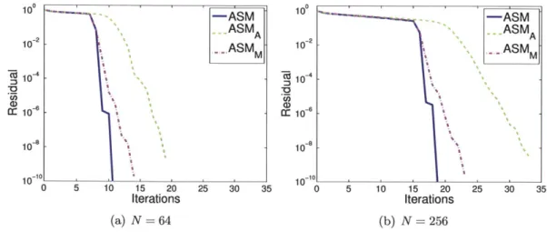
3-8 GMRES convergence history for advection-diffusion boundary layer problem with p = 10-6, p = 2 and n = 128 on isotropic structured mesh . . . . 48
4-1 Coarse basis functions for BDDC . . . . 59
4-2 Partially Assembled solve applied to sample Poisson problem . . . . 59
4-3 Effect of harmonic extensions for sample Poisson problem . . . . 59
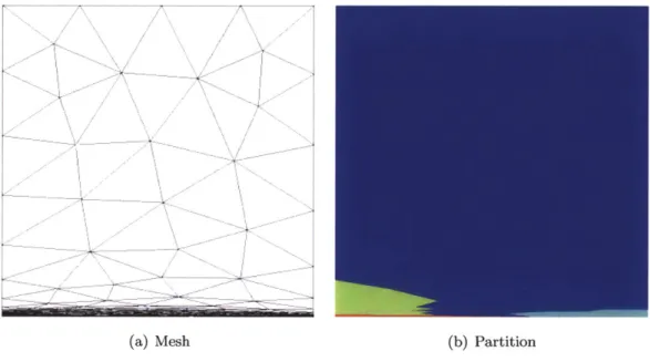
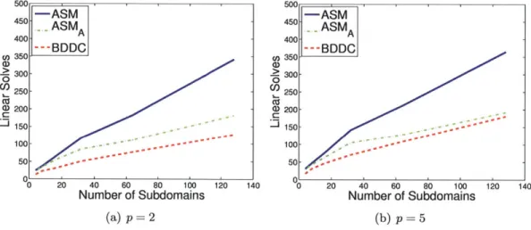
4-4 Unstructured mesh and partition for advection-diffusion boundary layer problem 70 4-5 Number of local linear solves for advection-diffusion boundary layer problem with y = 10~4, and n r 128 on anisotropic unstructured meshes . . . . 71
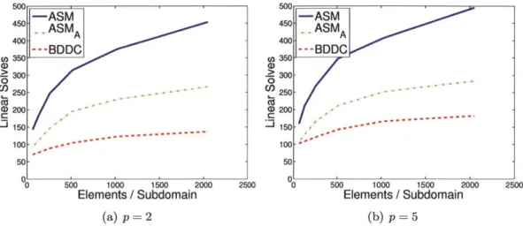
4-6 Number of local linear solves for advection-diffusion boundary layer problem with p = 10-4, and N = 64 on anisotropic unstructured meshes . . . . 72
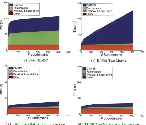
5-1 CPU time for 3D advection-diffusion boundary layer problem with p = 1, and n = 400 on isotropic unstructured mesh . . . . 98
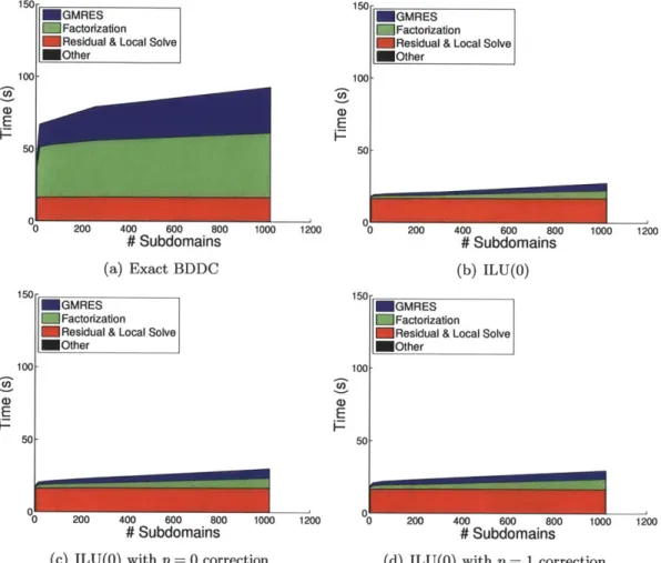
5-2 CPU time for 3D advection-diffusion boundary layer problem with P = 10-4, and n = 400 on isotropic unstructured mesh . . . . 99
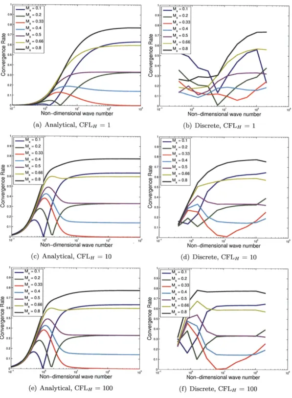
6-1 Convergence rate versus wave number, ( using basic Robin-Robin algorithm . 110 6-2 Optimization of asymptotic wave number . . . 112
6-3 Minimum asymptotic convergence rate . . . 112
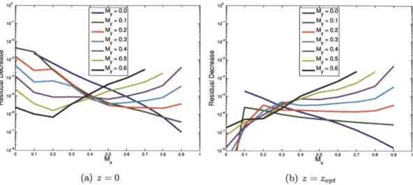
6-4 Convergence rate for different z, for M = 0.05, CFLH = 100 . . . . 113
6-5 Convergence rate for different z, for M = 0.05, CFLH = 100 . . . . 114
6-6 Optimization over all wave numbers . . . 115
6-7 Convergence rate using optimized interface conditions . . . 115
6-8 Discrete optimization of z . . . 116
6-9 Residual reduction for linearized Euler problem after 10 GMRES iterations . 117 6-10 Solution after one application of the BDDC preconditioner . . . 117
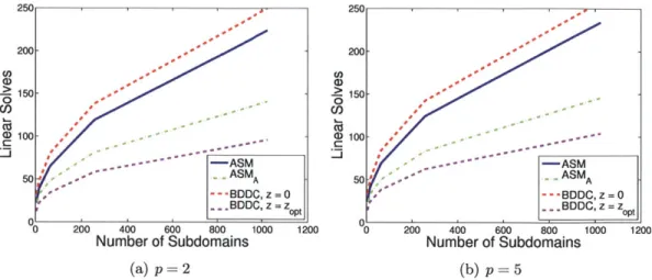
6-11 Number of local linear solves for linearized Euler problem with n = 512 . . . 119
6-12 Number of local linear solves for linearized Euler problem with N = 64 . . . . 119
6-14 Number of local linear solves for linearized Navier-Stokes problem, Re = 106 w ith n = 512 . . . 122 6-15 Number of local linear solves for linearized Navier-Stokes problem, Re = 104
w ith n = 512 . . . 122 6-16 Number of local linear solves for linearized Navier-Stokes problem, Re = 102
with n = 512 . . . .. . . . -. - - -. 123
6-17 Number of local linear solves for linearized Navier-Stokes problem, with p = 2 and N = 64 . . . .. . . .. . - - - . . . . 123 6-18 Number of local linear solves for linearized Navier-Stokes problem, Re = 0.01,
n= 512 ... ... . . . - - - . 125 6-19 Number of local linear solves for linearized Navier-Stokes problem, Re = 0.01,
N = 64 . . . .. . .. . . . . . 125 7-1 Grid and flow solution for inviscid flow over NACA0012, Moo = 0.3, a = 5.00,
p = 5 . . . ... . . . . .. . . . . ... . . . . . . . . 128
7-2 Weak scaling results for inviscid flow over NACA0012, Moo = 0.3, a = 5.00, p = 2, 2000 elements per subdomain . . . 129 7-3 Weak scaling results for inviscid flow over NACA0012, Moo = 0.3, a = 5.00,
p = 5, 500 elements per subdomain . . . 130
7-4 Detailed timing for inviscid flow over NACA0012, Moo = 0.3, a = 5.00, p = 5, 500 elements per subdomain . . . 131 7-5 Grid and flow solution for viscous flow over NACA0005, Mo = 0.2, a = 2.00,
Rec = 5000, p = 5 . . . 132
7-6 Weak scaling results for viscous flow over NACA0005, Moo = 0.2, a = 2.00,
Rec = 5000, p = 2, 1000 elements per subdomain . . . 132 7-7 Weak scaling results for viscous flow over NACA0005, Moo = 0.2, a = 2.00,
Rec = 5000, p = 5, 250 elements per subdomain . . . 133 7-8 Weak scaling results for inviscid flow over NACA0012, Moo = 0.3, a = 5.00,
p = 2, 2000 elements per subdomain . . . 136
7-9 Weak scaling results for inviscid flow over NACA0012, Moo = 0.3, a = 5.00,
p = 5, 500 elements per subdomain . . . 137
7-10 Weak scaling results for viscous flow over NACA0005, Mo. = 0.2, a = 2.0',
Rec = 5000, p = 2, 1000 elements per subdomain . . . 138 7-11 Weak scaling results for viscous flow over NACA0005, Moo = 0.2, a = 2.00,
Rec = 5000, p = 5, 250 elements per subdomain . . . 138 7-12 Grid and flow solution for turbulent flow over RAE2822, Moo = 0.3, a =
2.310, Rec = 6.5 x 10⁶, p = 2 . . . 139
7-13 Strong scaling results for turbulent flow over RAE2822, Moo = 0.3, a =
2.310, Rec = 6.5 x 10⁶, p = 2 adaptation step . . . 141
7-14 Weak scaling results for turbulent flow over RAE2822, Moo = 0.3, a = 2.310,
Rec = 6.5 x 10⁶, p = 2, 1000 elements per subdomain . . . 142 A-1 Analytical convergence rate versus wave number, ( using basic Robin-Robin
algorithm on two infinite domains . . . 160 A-2 Analytical convergence rate vs M,. using basic Robin-Robin algorithm on two
B-I Degrees of freedom involved in "local" bilinear form. *: Element Node, 0:
Neighbor Node, -*: Switch (3) . . . 168 B-2 Examples of subtriangulations of p = 1 triangular elements . . . 175
List of Tables
3.1 Number of GMRES iterations for Poisson problem on isotropic structured mesh 45 3.2 Number of GMRES iterations for advection-diffusion boundary layer problem
with p = 1 on isotropic structured mesh . . . 46 3.3 Number of GMRES iterations for advection-diffusion boundary layer problem
with p = 10-6 on isotropic structured mesh . . . 47 3.4 Number of GMRES iterations for advection-diffusion boundary layer problem
with p = 10-6 on anisotropic structured mesh . . . . 49 3.5 Number of GMRES iterations on both isotropic and anisotropic meshes with
N = 64,n = 128 . . . . 49
4.1 Number of GMRES iterations using BDDC preconditioner for Poisson prob-lem on isotropic structured mesh . . . 67
4.2 Iteration count for BDDC preconditioner with p = 1 or y = 1000, n = 128 . . 67
4.3 Number of GMRES iterations for advection-diffusion boundary layer problem with p = 1 on isotropic structured mesh . . . 68 4.4 Number of GMRES iterations for advection-diffusion boundary layer problem
with p = 10-6 on isotropic structured mesh . . . 68 4.5 Number of GMRES iterations for advection-diffusion boundary layer problem
with p = 10-6 on anisotropic structured mesh . . . 69 4.6 Number of GMRES iterations on both isotropic and anisotropic meshes with
N = 64,n = 128 . . . . 69
4.7 Number of local linear solves both isotropic and anisotropic meshes for scalar boundary layer problem with
p
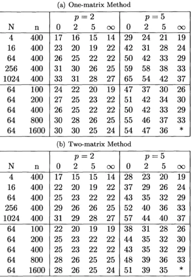
= 10~4 . . . . 72 5.1 Number of GMRES iterations for 3D Poisson problem using ILUT(T,7r)inex-act solver, with T = 10-6 and varying 7r . . . . 85
5.2 Number of GMRES iterations for 3D advection-diffusion boundary layer prob-lem with p = 1 on isotropic unstructured mesh using ILUT(r,7r) inexact
solver, with T = 10-6 and varying r . . . . 87 5.3 Number of GMRES iterations for 3D advection-diffusion boundary layer
prob-lem with p = 10-4 on isotropic unstructured mesh using ILUT(T,7r) inexact solver, with T = 10-6 and varying7r . . . . 88 5.4 Number of GMRES iterations for 3D Poisson problem using ILUT with p = 0
coarse grid correction, with r = 10-6 and varying
7r
. . . . 90 5.5 Number of GMRES iterations for 3D Poisson problem using ILUT(T,7r) with5.6 Number of GMRES iterations for 3D Poisson problem using ILUT(T,lr) with
p = 1 coarse grid correction applied to global partially assembled problem,
with T = 10-6 and varying r . . . . 92
5.7 Number of GMRES iterations for 3D advection-diffusion boundary layer prob-lem with y = 1, using ILUT(r,7r) with p = 0 coarse grid correction, with r = 10-6 and varying 7r . . . . 93
5.8 Number of GMRES iterations for 3D advection-diffusion boundary layer prob-lem with y = 1, using ILUT(r,lr) with p = 1 coarse grid correction, with T = 10-6 and varying 7 . . . . 94
5.9 Number of GMRES iterations for 3D advection-diffusion boundary layer prob-lem with p = 10-4, using ILUT(r,ir) with p = 0 coarse grid correction, with T = 10-6 and varying 7 . . . . 95
5.10 Number of GMRES iterations for 3D advection-diffusion boundary layer prob-lem with pa = 10- 4, using ILUT(r,lr) with p = 1 coarse grid correction, with T = 10-6 and varying r . . . . 96
5.11 Number of GMRES iterations for 3D advection-diffusion boundary layer prob-lem with p = 10~4, using ILUT(r,lr) with p = 1 coarse grid correction, with T = 10-6 and varying 7i . . . .. 100
6.1 Boundary Conditions . . . 104
6.2 Number of iterations required for the Schwarz algorithm to convergence using different interface and boundary conditions . . . 106
6.3 Number of iterations required for the Schwarz algorithm to convergence using characteristic interface conditions and different boundary conditions . . . 106
B.1 Numerical fluxes for different DG methods . . . 166
B.2 Numerical fluxes for different DG methods . . . 168
B.3 Elementwise bilinear form for different DG methods . . . 168
B.4 Iteration count for BDDC preconditioner using Interior Penalty Method . . . 179
B.5 Iteration count for BDDC preconditioner using the method of Bassi and Rebay180 B.6 Iteration count for BDDC preconditioner using the method of Brezzi et al. . . 180
B.7 Iteration count for BDDC preconditioner using the LDG method . . . 181
B.8 Iteration count for BDDC preconditioner using the CDG method . . . 181
B.9 Iteration count for BDDC preconditioner using the CDG method with p = 1 or 1000 ... ... 182
Chapter 1
Introduction
1.1
Motivation
Computational fluid dynamics (CFD) has advanced considerably in the past 30 years, such that CFD tools have become invaluable in the design and analysis of modern aircraft and spacecraft. CFD has become important due to the ability to simulate a large range of flow conditions at all relevant parameters in a flow (eg. Mach number, Reynolds number, specific heat ratio, etc.) which may not be possible in wind-tunnel experiments. Through advances in both numerical algorithms and computer hardware the complexity of problems solved has increased dramatically since the first two-dimensional potential flow simulations in the mid 1970s.
While the complexity of the problems has increased significantly, the desire to perform even more complex, higher-fidelity simulations remains. A recent review of the AIAA Drag Prediction Workshops shows that insufficient resolution remains a limiting factor in achiev-ing accurate predictions [84]. Aerodynamic flows involve features with a large range of spatial and temporal scales which need to be resolved in order to accurately predict desired engineering quantities. Higher-order methods provide a possible means of obtaining engi-neering required accuracy with fewer degrees of freedom. However, the requirements to have increased spatial and temporal resolution necessitates the use of more powerful computing resources.
Today's most powerful supercomputers are able to reach a peak performance of more than one petaflops. However, peak performance has been reached by a continuing trend of
parallelization, with the most powerful machines now employing more than 100,000 proces-sors. While several CFD codes have been used on large parallel systems with up to several thousand processors, the scalability of most CFD codes tops out around 512 cpus [89]. De-veloping CFD codes which are able to scale efficiently to tens or hundreds of thousands of processors remains a significant challenge.
1.2
Background
1.2.1
Higher-order Discontinuous Galerkin Methods
Higher-order methods have the potential for reducing the computational cost required to obtain engineering accuracy in CFD simulations. Typical industrial CFD methods employ second-order finite volume schemes for which the error scales as E c h2, where h is the
characteristic mesh size. Thus, in three dimensions, decreasing the mesh size by a factor of two leads to a four-fold reduction in solution error, but an eight-fold increase in the number of degrees of freedom. Higher-order numerical methods are those which achieve an error convergence E oc h', r > 2, provided the solution is sufficiently smooth. Thus, if a low error tolerance is required, higher-order methods allow for the error tolerance to be met with fewer degrees of freedom than typical second-order methods.
In this work a higher-order discontinuous Galerkin (DG) discretization is used [9, 11-14, 16, 37, 42, 56, 87, 97, 98]. DG methods are attractive since the piecewise discontinuous representation of the solution provides a natural means of achieving higher-order accuracy on arbitrary unstructured meshes. Even at high order, DG methods maintain a nearest-neighbour stencil as element-wise coupling is introduced only through the flux across element boundaries. In particular, this work uses a new DG variant known as the hybridizable discontinuous Galerkin (HDG) method [39-41, 96, 100]. In HDG methods, both the state variables and gradients are approximated on each element. As a result, HDG methods converge at optimal order (p+1) in both the state variables and gradients. Additionally, the state and gradient degrees of freedom may be locally eliminated to give a system of equations where the only globally-coupled degrees of freedom are associated with the trace values of the state variables on the element boundaries. Thus, for higher-order solutions HDG methods have much a smaller number of globally-coupled degrees of freedom compared to traditional
DG methods [41, 96].
1.2.2
Scalable Implicit CFD
A key use of massively parallel computers is to perform large-scale simulations in similar amount of time as typical industrial simulations on desktop machines. In addition to being able to partition the computational work among large numbers of processors, "optimal" algorithms are required for which the work scales linearly with the number of degrees of freedom. Two definitions of parallel scaling are commonly used: "strong scaling" and "weak scaling". Strong scaling, discussed in reference to Amdahl's Law [2], refers in general to parallel performance for fixed problem size, while weak scaling, discussed in reference to Gustafson's Law [61], refers to parallel performance in terms of fixed problem size per pro-cessor. While the parallel performance of a particular CFD code depends upon an efficient implementation, the performance is limited by the scalability of the underlying algorithm. Thus, this work focuses primarily on the algorithmic aspects to ensure scalability. In the context of high-fidelity CFD simulations, weak scaling is more important than strong scaling, as weak scaling relates closely to the ability of an algorithm to be optimal. Thus, unless oth-erwise stated the term "scalable" is used to imply "weakly scalable". An iterative solution algorithm is said to be scalable if the rate of convergence is independent of the number of subdomains into which the mesh has been partitioned, for a fixed number of elements on each subdomain. Thus, for a fixed number of elements on each subdomain, a scalable algorithm may be viewed as being optimal on a macro scale. A scalable algorithm is truly optimal if the rate convergence is also independent of the number of elements on each subdomain.
DG discretizations have long been associated with the use of explicit Runge-Kutta time integration schemes, due to the simplicity of implementation, relatively small memory re-quirements, and small stencils [42]. While explicit methods are relatively simple to imple-ment, the largest allowable time step is limited by the CFL condition, hence the number of iterations required for a particular simulation depends upon the mesh size. Thus, while explicit methods have the potential for very good strong scaling, these methods are not optimal. Implicit methods, on the other hand, do not have such a time step restriction. As a result, implicit methods have become the method of choice when the time step re-quired for numerical stability is well below that rere-quired to resolve the unsteady features
of the flow. Implicit schemes have also become widely used for the solution of steady-state problems obtained through pseudo-transient continuation [66], where time-stepping enables reliable convergence for nonlinear problems [3, 10, 26, 59, 60, 69, 83, 95, 122]. While most portions of an implicit code, such as residual and Jacobian evaluations, are trivially paral-lelized, implicit methods require at each iteration the solution of a globally coupled system of equations. Thus, implicit algorithms are optimal only if the globally coupled system may be solved in an optimal manner.
For aerodynamic problems, the most successful solution techniques have been nonlinear multigrid methods [3, 57, 82, 90, 93, 941 and preconditioned Newton-Krylov methods [59, 60, 69, 95, 103, 122]. Mavriplis showed that using a multigrid method as a preconditioner to a Newton-Krylov approach results in significantly faster convergence in terms of CPU time than a full nonlinear multigrid scheme [88]. Thus, in this work Newton-Krylov methods are considered, where the nonlinear system is solved using an approximate Newton method, while the linear system at each Newton iteration is solved using a preconditioned Krylov subspace method. In this context, multigrid methods may be viewed as one possible choice for the preconditioner. Thus, the development of an optimal solution method hinges on the ability to develop scalable preconditioners.
1.2.3
Domain Decomposition Theory
The desire to perform large scale simulations has led to an increased interest in domain decomposition methods for the solution of large algebraic systems arising from the dis-cretization of partial differential equations (PDEs). The term domain decomposition in the engineering community has often been used simply to refer to the partitioning of data across a parallel machine. However, data parallelism alone is insufficient to ensure good paral-lel performance. In particular, the performance of a domain decomposition preconditioner for the solution of large linear systems is strongly coupled to the discretization and the underlying PDE.
While high-fidelity simulations of aerodynamic flows involve solutions of the nonlinear compressible Euler and Navier-Stokes equations, performance of the algorithms developed for the systems resulting from the discretization of these equations are often analyzed in reference to simple scalar linear model equations for which the mathematical analysis is
possible.
Early aerodynamic simulations involved potential flow calculations. Thus, the Poisson equation has often been used as a model problem. In particular, the elliptic nature of the Poisson equation is appropriate for the analysis of acoustic modes in low speed, incom-pressible flows. Convective modes, on the other hand are hyperbolic and thus a convection equation is a more appropriate model for the analysis of these modes. A singularly per-turbed convection-diffusion equation is often used as a model problem for high Reynolds number compressible flows, where convective behaviour is dominant in most regions of the flow, while elliptic behaviour is dominant in the boundary layer region. Since much of the grid resolution is introduced in the boundary layer region, it is important to understand the elliptic behaviour present in these regions.
For elliptic PDEs, the Green's function extends throughout the entire domain decaying with increasing distance from the source. This implies that a residual at any point in the domain affects the solution everywhere else. In an unpreconditioned Krylov method, the application of the Jacobian matrix to a residual vector at each Krylov iteration exchanges information only to the extent of the numerical stencil. Thus, the number of iterations for an error to be transmitted across a domain of unit diameter is O(1), where h is the characteristic element size. In general, the convergence rate for symmetric problems is bounded by the condition number of the preconditioned system. An efficient preconditioner attempts to cluster the eigenvalues of the preconditioned system to ensure rapid convergence of the Krylov method. In particular, an efficient preconditioner for elliptic problems requires a means of controlling the lowest frequency error modes which extend throughout the domain. Domain decomposition methods precondition the system of equations resulting from the discretization of a PDE by repeatedly solving the PDE in subdomains of the original domain. If at each iteration information is exchanged only to neighbouring subdomains, the number of iterations for an error to be transmitted across a domain of unit diameter is O(1), where
H is the characteristic subdomain size. Thus the condition number of the preconditioned
system, and hence the number of iterations required to converge the linear system, will depend on the number of subdomains. In order to ensure that the condition number of the preconditioned system is independent of H scalable preconditioners include a coarse space able to control the low frequency error modes which span the entire domain [118].
While elliptic problems are characterized by Green's functions that extend throughout the entire domain, convection-dominated problems have a hyperbolic behaviour where the errors
propagate along characteristics in the flow. Thus, for convection-dominated problems, the resulting discretization is strongly coupled along the characteristics with little dissipation of errors across characteristics. Control of these errors is often accomplished by preconditioners that maintain strong coupling and often can be interpreted as increasing the propagation of errors out of the domain in the purely hyperbolic case.
For convection-diffusion problems, domain decomposition methods with a coarse space have been shown to be scalable, provided the diameter of the subdomains are sufficiently small [27, 29, 31]. Namely, if the Peclet number, defined using the subdomain length scale,
H, is sufficiently small, then the behaviour matches the symmetric, diffusion-dominated
limit. In the convection-dominated limit, the errors are propagated along characteristics in the domain. Thus, the number of iterations required to converge is proportional to the number of subdomains through which a characteristic must cross before exiting a domain.
In the case of unsteady convection-diffusion problems, solved using implicit time inte-gration, analysis of domain decomposition methods shows that a coarse space may not be necessary to guarantee scalability if the time step is sufficiently small relative the size of the subdomains [28, 30]. This behaviour may be interpreted using physical intuition. Namely, for small time steps the evolution of the flow is mostly local, thus a coarse space is not re-quired for the global control of error modes. From a linear algebra standpoint, the presence of the large temporal term leads to a diagonally dominant system, which tend to be easier to solve using iterative methods.
1.2.4
Large Scale CFD simulations
As aerodynamic flows involve both elliptic and hyperbolic features, the most successful serial algorithms have combined effective solvers for elliptic and hyperbolic problems. For example multigrid methods have been used in combination with tri-diagonal line solvers by Mavriplis and Pirzadeh [90] and Fidkowski et al. [57]. The success of these algorithms may be attributed to the ability of line solvers to control error modes in strongly coupled directions (either along characteristics or in regions of high anisotropy), while low frequency errors are corrected through the multigrid process. An alternative approach which appears
to be very successful for higher-order discretizations is a two-level method using an ILU(0) preconditioner with a minimum discarded fill ordering combined with a coarse grid correction presented by Persson and Peraire [103].
The development of efficient parallel preconditioners for aerodynamic flows builds upon successful algorithms in the serial context. While multigrid methods have been employed for large-scale parallel simulations, Mavriplis notes that special care must be taken in forming the nested coarse grid problems to ensure good performance [90, 94]. Domain decomposition preconditioners presented in this thesis may be viewed as two-level preconditioners, where local solvers are employed on each subdomain, while specially constructed coarse spaces are used to ensure the control of low frequency (global) modes throughout the domain.
The most widely used domain decomposition methods for CFD applications are addi-tive Schwarz methods [25, 32, 33, 35, 59, 60, 102, 122]. For cell-centered finite-volume, or higher-order discontinuous Galerkin discretizations, where degrees of freedom are naturally associated with element interiors, a non-overlapping additive Schwarz method corresponds to a subdomain-wise block-Jacobi preconditioner [45, 60, 102]. An overlapping additive Schwarz method may be developed by extending the size of the subdomain problems by layers of elements. Gropp et al. showed that adding a very small overlap corresponding only to a few layers of elements results in a significant improvement in the number of iterations required to converge a finite volume discretization of inviscid compressible flows [60]. How-ever, as increasing the amount of overlap lead to increased communication costs, the lowest CPU times were achieved using an overlap region of just two layers of elements. A variant presented by Cai et al, known as the restricted additive Schwarz method, updates only lo-cally owned degrees of freedom, eliminating communication during the solution update [35]. Numerical results have shown that this method actually requires fewer iterations to converge than the basic additive Schwarz preconditioner for both scalar convection-diffusion [35] and compressible Euler problems [33].
The use of domain decomposition methods for large scale applications involves additional considerations in order to achieve good performance. Large scale CFD applications may be both memory and CPU limited, making the exact solution of the local problems using LU factorization intractable. Thus, the local solvers are replaced with an iteration of an efficient serial preconditioner, such as an ILU factorization or a multigrid cycle. The performance
of the Schwarz method will, in general, depend upon the strength of the local solver. For example, Venkatakrishnan showed significant improvement using block-ILU(0) as opposed to block-Jacobi for the local solvers for an additive Schwarz method with zero overlap [122]. ILU factorizations have been particularly popular as local solvers for additive Schwarz methods with or without a coarse correction [25, 32, 33, 59, 60, 102, 122]. Cai, Farhat and Sarkis also employed a preconditioned GMRES method to solve the local problem on each subdomain [25, 32]. In particular, this allowed for different number of iterations to be used in each subdomain ensuring that each local problem was solved with sufficient accuracy.
For practical aerodynamic flows, the question remains whether a coarse space is neces-sary for a scalable preconditioner. For the solution of steady compressible Euler equations, Venkatakrishnan used a coarse space developed using an algebraic multigrid-type scheme [122]. In numerical simulations with up to 128 processors, Venkatakrishnan showed that the presence of the coarse grid gives some improvement in the performance of the preconditioner in terms of number of iterations, though this did not necessarily translate into faster solu-tion time. Gropp et al. did not employ a coarse space, and showed only modest increase in the number of linear iterations for strong scaling results from 32 to 128 processors [60]. In particular, Anderson, Gropp, and collaborators have performed large scale inviscid CFD simulations using over 3000 processors without employing a coarse space [4, 59, 60]. For unsteady simulations for the compressible Navier-Stokes equations, Cai, Farhat, and Sarkis found only a small increase in the number of iterations for strong scaling results up to 512 subdomains without the presence of a coarse space [25, 33]. Similarly, Persson showed good strong scaling performance up to 512 processors for the unsteady Navier-Stokes equations using a subdomain wise block-Jacobi preconditioner without a coarse space [102]. This ob-servation is consistent with the theoretical result for the time-dependent convection-diffusion problems, where a coarse space is not necessary if the time step is sufficiently small.
As the time step is allowed to increase, Persson showed that the performance of the pre-conditioner without a coarse space degrades significantly [102]. For steady state problems solved with little or no pseudo-temporal contributions, Diosady showed very poor strong scaling results using a similar preconditioner, particularly for viscous problems [45]. A par-titioning strategy weighted by the strength of the coupling between elements was introduced in order to improve the parallel scaling of this preconditioner [45]. A similar strategy was
also employed by Persson [102]. However, the resulting partitions had larger surface area to volume ratios resulting in more communication per computation. While such a technique improves parallel performance on a moderate number of processors, the use of a coarse space may be essential for obtaining a scalable method for steady state viscous flow problems on massively parallel systems.
Inexact Schur complement methods have been used as an alternative means of obtaining a global correction for CFD simulations [10, 64]. Schur complement methods reduce the size of the global system to a system corresponding only to the degrees of freedom on ( or near ) the interfaces between subdomains. Inexact Schur complement methods solve an approximate Schur complement problem in order to precondition the global system. The solution of the approximate Schur complement problem acts as a global coarse grid correction. For example, Barth et al. developed a global preconditioner based on an approximate Schur complement for the solution of the conforming finite element discretization of the Euler equations, where approximate Schur complements were computed using ILU preconditioned GMRES [10]. Similarly, Hicken and Zingg developed a preconditioner for a finite-difference discretization of the compressible Euler equation by computing an approximate Schur complement using an ILU factorization. Both Barth et al. and Hicken and Zingg used a preconditioned GMRES method to iteratively solve the inexact Schur complement system leading to non-stationary preconditioners which were applied to the flexible variant of GMRES [109]. While much smaller than the entire global system, the Schur complement system is still globally coupled and an effective preconditioner for the Schur complement problem requires a coarse space in order to effectively control the low frequency error modes.
1.2.5
Balancing Domain Decomposition by Constraints
In order to solve the Schur complement problem, this work considers a class of domain decomposition preconditioners known as Neumann-Neumann methods which were originally developed to solve elliptic problems [21, 44, 116]. While all of the methods discussed have defined local problems based on blocks of the fully assembled discrete system, Neumann-Neumann methods exploit the finite element residual assembly to define the local problem. While the original Neumann-Neumann methods lacked a coarse space, Mandel introduced a coarse space leading to the Balancing Domain Decomposition (BDD) method [73, 74].
The BDD method was later shown to be closely related to the Finite Element Tearing and Interconnecting (FETI) method [54, 58]. FETI methods are among the most widely used and well tested methods for structural mechanics problems. For example Bhardwaj et al. used FETI methods to solve structural mechanics problems on up to 1000 processors [18]. The most advanced of the FETI and Neumann-Neumann class of methods are the dual-primal FETI (FETI-DP) [53, 80] and the Balancing Domain Decomposition by Constraints (BDDC) method [47, 75]. Like FETI and BDD, FETI-DP and BDDC methods are closely related and have essentially the same eigenvalue spectra [71, 76]. The analysis of these preconditioners have been extended to the case where inexact local solvers are used in [48, 67, 72]. Additionally, several authors have presented multi-level versions of the BDDC method [78, 79, 120]. An adaptive method for adding primal degrees of freedom to ensure rapid convergence has also been presented[77]. Practical implementations of the FETI-DP method has been used to solve structural mechanics problems on up to 3000 processors
[19, 104].
While originally developed for elliptic problems, Achdou et al. modified the Neumann-Neumann interface condition to Robin-Robin interface conditions for a convection-diffusion problem, ensuring that the local bilinear forms were coercive [1]. A Fourier analysis, on a partitioning of the domain into strips normal to the stream-wise direction, showed that in the convective limit, the resulting algorithm converges in a number of iterations equal to half the number of subdomains in the stream-wise direction. The Robin-Robin interface conditions have been used along with a FETI method to solve linear convection-diffusion problems by Toselli [117]. Similarly, Tu and Li used the Robin-Robin interface condition to extend the BDDC method to convection-diffusion problems [121].
Neumann-Neumann and FETI methods have in general not been used for large scale CFD simulations, however recent work is beginning to make these methods available to the systems of equations for compressible flows. Dolean and collaborators have extended the Robin-Robin interface condition to the isentropic Euler equations using a Smith factorization [50, 51]. Yano and Darmofal also provided a generalization of the Robin-Robin interface condition to the Euler equations based on entropy symmetrization theory [123, 124]. However, detailed analysis of the performance of this algorithm has yet to be performed.
1.3
Thesis Overview
1.3.1
Objectives
The objective of this work is to develop a scalable high-fidelity solver for higher-order dis-cretizations of convection-dominated flows. In order to meet this objective, this work presents a solution strategy based on an implicit Newton-Krylov method using domain decomposition preconditioners.
1.3.2
Thesis Contributions
The contributions of this thesis are the following:
o An additive Schwarz preconditioner with a coarse space based on harmonic extensions is developed for higher-order hybridizable discontinuous Galerkin discretizations. The coarse space correction is shown to improve the convergence relative to a single level additive Schwarz preconditioner for convection dominated flows solved on anisotropic meshes.
o A Balancing Domain Decomposition by Constraints (BDDC) preconditioner is devel-oped for higher-order hybridizable discontinuous Galerkin (HDG) discretizations. The BDDC method is proven to converge at a rate independent of the number of subdo-mains and only weakly dependent on the solution order and the number of elements per subdomain, for a second-order elliptic problem. The BDDC preconditioner is extended to the solution of convection-dominated problems using a Robin-Robin interface con-dition. Numerical results show that the BDDC preconditioner reduces the number of local linear solves required to converge relative the additive Schwarz preconditioner with or without coarse space for convection-dominated problems solved on anisotropic meshes.
o An inexact BDDC preconditioner is developed based on incomplete factorizations and a p-multigrid type coarse grid correction. It is shown that the incomplete factorization of the singular linear systems corresponding to local Neumann problems results in a non-singular preconditioner. Numerical results show that the inexact BDDC precon-ditioner converges in a similar number of iterations as the exact BDDC method, with
significantly reduced CPU time.
" An analysis is performed to assess the effect of far-field boundary conditions on the convergence of domain decomposition methods for the compressible Euler equations. It is shown that, even in the one-dimensional case, applying reflecting boundary con-ditions leads to exponential convergence (as opposed to convergence in a finite number of iterations).
"
The BDDC preconditioner is extended to the solution of the compressible Euler equa-tions using optimized interface condiequa-tions. Numerical results show that the optimized interface conditions significantly improve the performance of the BDDC preconditioner relative to the standard Robin-Robin interface condition." A restricted overlapping Schwarz preconditioner is developed for a higher-order dis-continuous Galerkin (DG) discretization of the compressible Euler and Navier-Stokes equations. It is shown that using an overlap of consisting of only a single layer of elements significantly improves relative to a non-overlapping preconditioner.
" A BDDC preconditioner is developed for a large class of higher-order discontinuous Galerkin discretizations. The BDDC method is proven to converge at a rate indepen-dent of the number of subdomains and only weakly depenindepen-dent on the solution order or the number of elements per subdomain, for a second-order elliptic problem.
The thesis is organized as follows. Chapter 2 presents the HDG discretization. Chapter 3 presents the domain decomposition and develops the additive Schwarz preconditioner. Chapter 4 introduces the BDDC preconditioner, while Chapter 5 presents an inexact variant of the BDDC preconditioner. Chapter 6 provides an analysis of the performance of the domain decomposition preconditioners for the Euler and Navier-Stokes systems of equations.
Chapter 7 presents numerical results for several fundamental aerodynamic flows. Finally, Chapter 8 gives conclusions and recommendations for future work.
Chapter 2
Discretization and Governing
Equations
2.1
HDG Discretization
The hybridizable discontinuous Galerkin discretization is presented for a general system of conservation equations. Let u(x, t) : Rd x R+ --+ Rm be the vector of m-state variables in d-dimensions. A general conservation law in a physical domain, Q C Rd, d - 2,3, is given
by:
Uk,t + (Fik(U) + Gik (U, U,x)),X, = fk(ujuXx),
where k
C
{1, ... , m} is the component index of the governing equations, i E {1, ... , d} isthe spatial index, (-),t is the temporal derivative, and (.),x, is the spatial derivative with
respect to xi. F(u) : R' --+ Rmxd and G(u, u,x) : Rm x Rmxd -> Rmxd are the viscous and inviscid fluxes, respectively. (2.1) may be rewritten as the following first order system of equations:
qik - Uk,x, = 0
Uk,t + (Fik(u) + Gik(u, q)),x,
(2.2)
(2.3) (2.1)
The HDG discretization is obtained from a weak form of (2.2)-(2.3). Let the tessellation Th be a partition of Q into triangles or quadrilaterals (if d = 2) or tetrahedra or hexahedra (if d = 3). Define E to be the union of edges (if d = 2) or faces (if d = 3) of elements, K. Additionally, define FInt c S and Ea C E to be the set of interior and boundary edges, respectively. Any
edge e E gInt is shared by two adjacent elements K+ and n~ with corresponding outward pointing normal vectors n+ and n-.
Let PP(D) denote the space of polynomials of order at most p on D. Given the tessellation
Th, define the following finite element spaces:
Vh := {v E
(L2(Q))mx
: Vl6 E (pP(,))mxd V E T (2.4)W {w E (L2(Q))m :
wI,
E (PP()) m Vs E T} (2.5)M
:={ E
(L2(,)) m :yMe E
(PP(e))m VeE E}.
(2.6)Consider the steady state solution to (2.2)-(2.3). The weak form is given by: Find
(q, u) E VP x Wh such that for all K E Th,
(qi, Vi -+ (U, vik,x) - (i, Vikfni)a.
=
0 Vv E (2.7)-(Fik (U) + Gik (u, q), kxW),r + (i - Gik) ni, Wk
=
(fk, Wk) K Vw E W, (2.8)where (w, v), :=
f,
wV and (w, v)aK := fa, wv. In the case of unsteady problems, or steadyproblems driven to steady-state using pseudo-transient time continuation, (2.8) also includes temporal terms appropriate to the time stepping scheme used. In (2.8), (Fik + Gik)ni is the numerical flux which approximates (Fik (u) + Gik(u, q))ni on On, while it E MhP approximates the trace of u on E. The numerical flux takes on the form:
( -+-
SG~)ni
= (Fik (f) + Gik (t, q))ni + Ski(ft, n)(ul - fit) on OK, (2.9)where S(fi, n) is a local stabilization matrix. The local stabilization matrix has the form:
S(ft,n) = |An|+SDiff, (2.10)
coefficients of the diffusive terms [39].
Elements in the HDG discretization are coupled by ensuring that the numerical flux is continuous across faces in 9l"t. Specifically, the HDG discretization enforces that the jump in the numerical flux, (Fik + Gik)nt
+
(+ k +Sik)-n-,
between elements n,+ andK- is orthogonal to all functions in M(EInt). Summing over all element gives the HDG discretization: Find (q, u, fi) E VP x W' x MI such that
(qik, vik)T + (Uk, vik,xi)T (ilk, vikni)ar 0 Vv
C
VP (2.11)(Fik(U) + Gik
(u,
q), Wkxx)r +K(ik
+ Gik) ni, Wk) = (f, Wk)T Vw E WhP (2.12)(Fik + Gik)ni, P/k)aT\a = 0 VA E Mhi (2.13)
Bk, Ak = 0 Vp E Mp,, (2.14)
where (-, -)r :=Eer(, - (-, )T : KCr (-, .)a and (-, -)ar\an := EKET (-, -)a\a,
while M and M'~a are subsets of MhP corresponding to edge functions interior to Q and on 8Q, respectively. B is a boundary term used to enforce the desired boundary conditions on
8Q. The specific form of B for different types of boundary conditions is discussed in Section
2.3. Specifying a basis for V(, Wh and Mh, (2.11) - (2.13) leads to a non-linear system of equations for the coefficients of the basis functions. Applying Newton's method results in a discrete linear system at each Newton iteration of the form:
Aqq Aqu Aqx AqAb Aq bq
Auq Auu Au\ AuAb Au (2.15)
AAq AAu AA\ AAAb A
b\
AAbq AAbu AAbAb AAbAb _ Ab _ bAb J
where Aq, Au, A, Ab denote the vector of updates for the coefficients of basis functions
corresponding to q, u and fi on e E EInt and e E S' respectively. The system (2.15) has an element-wise block diagonal form such that Aq, Au and Ab in (2.15) may be eliminated element by element to get the following system:
where
Aqq
Aqu
AqAgAqA
A
-[
AxqA,
AAAbAuq
AUU
AuAb
Au.
(2.17)
A
A
AAbu
nq
AAbAb
A A
Aqq Aqu AqAb bq
b
=
b,
-[
AqAA\u AAAb
AuqAU
AuAb
b
.(2.18)
AAbq
AAbu AAbAb
bAbThe superscript in A is used to denote the globally assembled finite element matrix consistent with the notation in Chapter 4. Alternatively, A = Afi may be viewed as the solution of linearized form:
a(A,
p)
= b(p) VE
M, (2.19)where a(A, p) and b(t) are given by:
a(A,
p)
=
a (A,
y) =(AZF ' + AGik)ni, p
(2.20)
KET nET
b(,p)
=
b. (/p) =
(F'
+ AGR)n,)
(2.21)
nET r-ET
Here, (AF1I
+
AGj)nj
is the change in numerical flux obtained by solving the linearized problem about (q, f) corresponding to (2.7) - (2.8) with Aft = A and zero right-hand side. Similarly, (AE"R'+ A50 )nj is the change in numerical flux obtained by solving the linearized problem with Aft = 0 and right-hand sides corresponding to the residual of (2.7) - (2.8) at the linearization point.2.2
Compressible Navier-Stokes Equations
The compressible Euler and Navier-Stokes equations are systems of non-linear conserva-tion equaconserva-tions of the form (2.1). In particular, the Euler equaconserva-tions are obtained from the Navier-Stokes equations by setting the viscous flux vector to zero and omitting (2.11) for the gradient. The conservative state vector is given by u = [p, poi, pE]T, where p is the density,
vi the velocity in direction i, and E the total internal energy. The inviscid flux vector is given by:
p[i
F(u) = pViVj + ijp
pvH
(2.22)
where p is the static pressure, H = E + P is the total enthalpy, and
oij
is the Kroneckerp
delta:
6ij
=
i-otherwise.
(2.23)
The pressure is given by:
p = (y - 1)p E - 1pvivi), (2.24)
where -y is the specific heat ratio (y = 1.4 for air). The viscous flux vector is given by:
Gi(u, u,x) =
0
Tij
vjrij + nTT,xJ
where r is the shear stress tensor, nT is the thermal conductivity, T = p/pR is the
temper-ature, and R is the gas constant. The shear stress tensor, -r, is given by:
rij = P(vi,x + Vj,x) - 6ijAVk,xk, (2.26)
where pL is the dynamic viscosity and A = 9P is the bulk viscosity coefficient. The dynamic viscosity is given by Sutherland's Law:
T ( Tref + Ts
Tref T+Tq (2.27)
The thermal conductivity is a function of the dynamic viscosity:
Kr =
ypR
,(2.28)('y- 1)Pr'
where Pr is the Prandtl number. For air, Tref = 2880 K, T, = 110.4' K and Pr = 0.71.
2.3
Boundary Conditions
This section gives the exact form of the boundary term B used to define various boundary conditions for the compressible Euler and Navier-Stokes equations.
Flow Tangency BC
A slip boundary condition is enforced on a symmetry plane or at a solid surface in inviscid flow. The boundary condition may be written as:
p -p
$
=
poi-(PVkk)ni-
pi
(2.29)
pE - pE
where pvknk is the normal component of the velocity. Thus setting B = 0 weakly enforces
p, pE = pE, and p'Vi has zero component in the normal direction (since pVi - (pVknk)ni
is the interior momentum with the normal component removed).
Adiabatic No-slip BC
At a solid surface for viscous flow an adiabatic no slip boundary condition is set by enforcing zero velocity and heat flux. Namely, the boundary condition is written as:
(Fil
+
Gil)f3= pii (2.30)
(Fim + Gim)
The first condition enforce zero mass flux through the boundary, the second condition ensures zero momentum at the surface, while the third condition ensures the heat flux into the
domain is zero.
Isothermal No-slip BC
In order to set an isothermal no slip boundary condition at a solid surface for viscous flow, the boundary condition is similar to the adiabatic no slip condition except the last component of the boundary condition is set to T - T(fi). T, is the desired surface temperature and T(ni) is the temperature computed as a function of fi.
Characteristic Inflow/Outflow BCs
At an inflow/outflow boundary, a free-stream condition, u,, is specified and the boundary condition is given by:
B =
[(Fi
+ Oj)nji
- [Fi(f)ni+
An(u, - u) + (Ginj),]. (2.31)where An = 9(Fi(ft)ni)/8(i), with A± = (An ±
IAn|)/2.
Here (Ginj), is a specified normal viscous flux at the boundary, usually assumed to be zero. This choice of B ensures that the mathematically correct number of boundary conditions are specified at inflow and outflow boundary conditions. Namely, for two-dimensional subsonic inviscid flow three inflow and one outflow boundary conditions are set, while for viscous flow four inflow and three outflow conditions are set [62]. In the case of inviscid flow this boundary condition simplifies to the expression given by Peraire et al. [100]:a
= A+(u - f) - A-(u - fi) (2.32)Other Inflow/Outflow BCs
It is often convenient to specify inflow and outflow BCs without complete knowledge of the boundary state. For example total pressure, total temperature and angle of attack may be specified at an inflow boundary or a desired static pressure may be specified at an outflow boundary. For these types of boundary conditions, a boundary state u is reconstructed as a function of the interior state u and the desired boundary condition. The boundary flux B is then set in the same manner as the characteristic the BCs given above.