HAL Id: hal-02592964
https://hal.inrae.fr/hal-02592964
Submitted on 15 May 2020
HAL is a multi-disciplinary open access archive for the deposit and dissemination of sci-entific research documents, whether they are pub-lished or not. The documents may come from teaching and research institutions in France or
L’archive ouverte pluridisciplinaire HAL, est destinée au dépôt et à la diffusion de documents scientifiques de niveau recherche, publiés ou non, émanant des établissements d’enseignement et de recherche français ou étrangers, des laboratoires
European Fish Index Deliverable 4.1 : Report on the
modelling of reference conditions and on the sensitivity
of candidate metrics to anthropogenic pressures.
Deliverable 4.2: Report on the final development and
validation of the new European Fish Index and method,
including a complete technical description of the new
method. 6th Framework Programme Priority
FP6-2005-SSP-5-A. N° 0044096. Rapport final
Didier Pont, P. Bady, M. Logez, J. Veslot
To cite this version:
Didier Pont, P. Bady, M. Logez, J. Veslot. EFI+ Project. Improvement and spatial extension of the European Fish Index Deliverable 4.1 : Report on the modelling of reference conditions and on the sensitivity of candidate metrics to anthropogenic pressures. Deliverable 4.2: Report on the final de-velopment and validation of the new European Fish Index and method, including a complete technical description of the new method. 6th Framework Programme Priority FP6-2005-SSP-5-A. N° 0044096. Rapport final. [Research Report] irstea. 2009, pp.179. �hal-02592964�
SIXTH FRAMEWORK PROGRAMME
PRIORITY FP6-2005-SSP-5-A
“Integrating and Strengthening the European Research Area” – “Scientific
Support to Policies”
Project no.: 0044096
Project acronym: EFI+
Improvement and spatial extension of the European Fish Index
Instrument: STREP
Thematic Priority: Scientific Support to Policies (SSP) - POLICIES-1.5
WORKPACKAGE 4
Deliverable 4.1: Report on the modelling of reference conditions and on the
sensitivity of candidate metrics to anthropogenic pressures
Deliverable 4.2: Report on the final development and validation of the new
European Fish Index and method, including a complete technical description of the
new method.
Authors:
Pierre Bady*, Didier Pont*, Maxime Logez**, Jacques Veslot**
* CEMAGREF (HBAN), Parc de Tourvoie, BP 44, 92163 Antony Cedex, FRANCE
** CEMAGREF (HYAX), 3275 Route de Cézanne, CS 40061, 13182 AIX EN PROVENCE Cedex 5, FRANCE
Keywords: EFI+, Fish index, multimetric index, modelling procedure, model, GLM, scoring, prediction, diagnostic, goodness of fit, predictive error, zonation, spatial organisation, metric aggregation.
Contents
Summary and recommendations ... 4
1 Introduction ... 21
2 Environmental and biological Data... 23
2.1 Dataset Description ... 23
2.1.1 Global description of the dataset... 23
2.1.2 Description of the calibration (CD) dataset and description of the slightly disturbed dataset (SID)... 25
2.1.3 Spatial organization (regionalization and zonation)... 29
2.1.3.1 Ecoregion typology ... 30
2.1.3.2 River zonation ... 31
2.1.3.3 Combined typology ... 35
2.1.3.4 Match between river typology and relative abundance of salmonid-type species (undisturbed sites)... 36
2.1.4 Pressure indices ... 37
2.2 Environmental Variables for modelling... 40
2.3 Functional guilds and metrics ... 44
3 Metric Modelling... 46
3.1 Statistical models... 46
3.1.1 Model description... 46
3.1.2 Diagnostic and goodness of fit ... 47
3.1.3 Implementation... 49
3.2 Metric based on species number ... 49
3.2.1.1 Species intolerant to low Oxygen Concentration (Ric.O2.Intol) ... 50
3.2.1.2 Species intolerant to Habitat degradation (Ric.Hab.Intol) ... 51
3.2.1.3 Rheophilous Species (Ric Hab RH) ... 53
3.2.1.4 Insectivorous Species (Ric INSV)... 54
3.2.1.5 Species with preference to spawn in running waters (Ric RH Par) ... 56
3.3 Metric based on fish number... 57
3.3.1.1 Fish intolerant to low Oxygen Concentration (Ni.O2.Intol) ... 57
3.3.1.2 Fish intolerant to Habitat degradation (Ni.Hab.Intol) ... 59
3.3.1.3 Insectivorous Fish (Ni.INSV) ... 60
3.3.1.4 Lithophilic Fish (Ni.LITHO)... 62
3.4 Metrics based on Fish Length ... 63
3.4.1 Environmental variables and data sets definition... 64
3.4.1.1 Experiment on the brown trout, Salmo trutta fario. ... 65
3.4.1.1.1 Developing a tool to estimate the cut-off between young of the year and older fishes ... 65
3.4.1.1.2 Definition of metrics ... 65
3.4.1.1.3 Selection of calibration data set ... 65
3.4.1.1.4 Modelling of metrics ... 65
3.4.1.2 Crossing metrics based on guilds and size classes... 66
3.4.1.2.1 Definition of metrics ... 66
3.4.1.2.2 Selection of calibration data set ... 67
3.4.1.2.3 Specific Modelling of metrics ... 67
3.4.1.3 Brown trout experiment ... 67
3.4.1.3.1 Environment of the calibration data set for the metrics ... 68
3.4.1.4 Crossing metrics and size class ... 71
3.4.1.4.1 Metrics selected... 71
3.4.1.4.2 Environment of the calibration data set... 71
3.4.1.4.3 Modelling of the four selected variables ... 72
3.4.2 Discussion ... 78
3.5 Conclusion... 79
4 Metric selection ... 81
4.1 Introduction ... 81
4.2 Metric computation ... 81
4.2.1 Standardization per ecoregion and river zone ... 81
4.2.2 Rescaling between 0 and 1 ... 83
4.3 Metric selection ... 83
4.3.1 Correlations between candidate metrics... 83
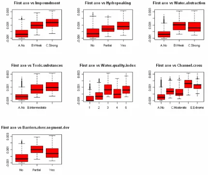
4.3.2 Sensitivity to pressures... 84
4.3.3 Representativeness of guilds and metrics... 87
4.3.4 Final metric selection ... 88
5 Metric Aggregation, Scoring and Performance analyses ... 88
5.1 Index definitions... 88
5.1.1 Indices definition per river zone... 88
5.1.2 Efficiency of the river type classification ... 90
5.1.3 Limitations of the index ... 94
5.1.3.1 Sensitivity of the indices to the sampling method... 94
5.1.3.2 Sensitivity of the index to the sampling strategy ... 95
5.1.3.3 Sensitivity of the index to the number of fish caught ... 96
5.1.3.4 Sensitivity of the index to specific environmental situations... 97
5.1.3.5 Case of large rivers... 99
5.1.3.6 Sensitivity of the index to the species richness ... 101
5.1.4 Conclusion and recommendation ... 102
5.1.4.1 River zonation classification ... 102
5.1.4.2 Limitation of the Index in relation with the environment ... 105
5.1.4.3 Limitations in the use of the Index due to the number of fish caught... 105
5.1.4.4 Limitations in the use of the Index due to the sampling method ... 106
5.1.5 Scoring in 5 classes ... 106
5.2 Performance analyses... 108
5.2.1 Tools and concepts ... 108
5.2.2 Evaluation classification ... 109
5.2.3 Classification and optimisation ... 111
5.2.4 Conclusion... 113
6 How estimate the error of multi-metric index based on modelling step: an proposition114 6.1.1 Confidence and Prediction Intervals ... 114
6.1.2 Simulation of tolerance intervals for individual score ... 115
6.1.3 Predictive error after metric aggregation ... 116
7 References ... 118
8 Annexes... 123
8.1 Biological variables descriptions (guilds and traits) ... 123
8.2 Computation of the Habitat Index, water alteration and Channel-Crossection variables. ... 127
8.2.1 Habitat Index ... 127
8.2.2 Water alteration Index... 127
Summary and Recommendations
Objectives
The European Fish Index (EFI) is a multimetric index based on a predictive model that derives reference conditions from abiotic environmental characteristics of individual sites and quantifies the deviation between the predicted fish community (in the “quasi absence” of any human disturbance) and the observed fish community (described during a fish sampling occasion). The metrics used are based on species guilds describing the main ecological and biological characteristics of the fish community.
The objective of the index is to evaluate the ecological status of sites at the European scale. One of our main objectives during the development phase was to define a calibration dataset (to calibrate models) and to model and select metrics in a way that the index could be correctly calibrated for all or most of ecoregions and environmental situation, i.e. in the absence of any significant pressures, the index values must be high (close to 0.80) and comparable between ecoregion, river zone and local environment. The sensitivity of the final indices to morphological pressures has to be considered first at such large scale.
In the same way, and at the opposite of the previous European index (FAME project), the ecological classes boundaries are based on the distributions of indices values for undisturbed sites in two types of rivers (see below). In other words, the main objective was to optimize first the specificity (capacity of the indices to correctly classify an undisturbed site as undisturbed, i.e. with a high index value) and in a second step the sensitivity (i.e. the capacity of the indices to detect the effect of a pressure).
Two indices, each composed of 2 different metrics, can be computed depending of the river zone classification of a given site:
- Salmonid Dominated Fish Assemblage Index (Salm.Fish.Index) for sites classified as Salmonid Dominated Fish Assemblage River Type (Salmonid river zone)
- Tolerant Fish Assemblage Index (Cypr.Fish.Index) for sites classified as Cyprinid Dominated Fish Assemblage River Type (Cyprinid river zone)
Salm.Fish.Index = (Ni.Hab.150 + Ni.O2.Intol) / 2 Cypr.Fish.Index = (Ric.RH.Par + Ni.LITHO) / 2
Metric names Detailled names
Ric.RH.Par Rheophilic reproduction habitat species richness
Ni.O2.Intol Oxygen depletion intolerant species abundance (Nb. individuals) Ni.LITHO Lithophilic reproduction habitat species abundance (Nb. Individuals) Ni.Hab.Intol.150 Abundance of individuals < 15 cm of Habitat intolerant species
One metric is expressed in term of richness, two in abundance of individuals and one in abundance per size class. Two metrics are based on tolerance responses, and two on reproduction. The four metrics decrease when exposition to human pressures increases. The correlations between metrics are relatively low (Pearson’s coefficients less than 0.65)
Species classified as oxygen depletion intolerant, habitat alteration intolerant, lithophilic and rheophilic reproduction habitat are listed in Annex.
The final scoring is presented below in the Method description section.
The distinction between the 2 river types is based on the proportion of typical species belonging to Salmonid dominated fish communities (or Salmonid type species) - denominated ST-species - which are oxygen depletion intolerant, habitat alteration intolerant, stenothermic, lithophilic or speleophilic reproduction type species and with a rheophilic reproductive habitat. These 19 species are the following:
Alburnoides.bipunctatus Cobitis.calderoni Coregonus.lavaretus
Cottus.gobio Cottus.poecilopus Eudontomyzon.mariae
Hucho.hucho Lampetra.planeri Phoxinus.phoxinus
Salmo.salar Salmo.trutta.fario Salmo.trutta.lacustris Salmo.trutta.macrostigma Salmo.trutta.trutta Salmo.trutta.marmoratus Salvelinus.fontinalis Salvelinus.namaycush Salvelinus.umbla
Thymallus.thymallus
List of intolerant species typically belonging to Salmonid dominated fish communities Typically, an undisturbed salmonid river type site is dominated by ST-species which represent more than 80% of the number of individuals caught (more than 90 % most of time). At the opposite, the relative abundance of these species is less than 20% (most of time 10%) for a typical cyprinid type site.
Due to the fact that human pressures impact significantly the fish community structure, it is not possible to directly use this fish community based criteria to discriminate between salmonid type sites and cyprinid type sites. A solution to classify the sites was to use a typology based on abiotic variables. Melcher et al. (2007) produced such a typology at the European scale during the FAME project (EFT classification). Using 7 environmental variables, the authors differentiate between 15 fish-based river types. These types can be gathered in our two main river types, considering our criteria related to the relative abundance of ST-species.
This typology has been used during the process of metric standardization and selection. Nevertheless, in several situations, sites are misclassified:
- Some undisturbed sites classified as cyprinid river zone sites have a high relative abundance of ST-species.
- At the opposite, but more seldom, undisturbed sites classified as salmonid river zone site have a too low relative abundance of typical upstream intolerant species. Then the proportion of upstream intolerant species has to be evaluated by the user a posteriori to check the correctness of the river type proposed for each site and to attribute the correct index to the considered site (Salm.Fish.Index or Cypr.Fish.Index). Depending of the situation (see after), recommendations are given to the user.
The general description of the method is first summarized, followed by the limitations of the 2 indices, the procedure used for metric modelling, metric selection and standardisation. Finally, the main results related to indices performance (specificity versus sensitivity) and evaluations of uncertainties are presented.
Method description:
The procedure is summarized in Figure a. Each number (from 1 to 7) refers to one of the different steps of the procedure presented below.
1. Data needed
EFI+ uses 2 types of data.
- Data from single-pass electric fishing catches to calculate the assessment metrics. Individuals have to be measured separately (to the next mm) to compute the observed values of the metrics. The results are given in number of individual caught per species.
- variables describing environment at the site scale or river segment scale, and the sampling method (Tables b and c).
- Additional information on location (longitude and latitude), site name and sampling date is required.
Ecoregion classification is the one of Illies, but with the addition of a Mediterranean region. Spatial coordinates are used to define the corresponding ecoregion.
Figure b. Flow chart describing the procedure. Green rectangles: input data and end-user intervention. Pink rhomb: computation and process. Yellow hexagon: intermediate results available in the software output. Blue oval: fish index value and ranking in five classes.
One-Pass Fish sample (1) Spatial Coordinates (1) Environmental Characteristics (1) Sampling method Ecoregion (2) Intolerant ST-Species % Ind. Observed Metric Values(4) Predictive Models (3) Expected Metric Value (3) River Type (2) Residual Standardization (4) Re-scaling (5) Metric Scores(5) Salmonid fish Index (6) Cyprinid fish Index (6) Index selection (6) Fish Index value and Ranking (7) End- User Agreement One-Pass Fish sample (1) Spatial Coordinates (1) Environmental Characteristics (1) Sampling method Ecoregion (2) Intolerant ST-Species % Ind. Observed Metric Values(4) Predictive Models (3) Expected Metric Value (3) River Type (2) Residual Standardization (4) Re-scaling (5) Metric Scores(5) Salmonid fish Index (6) Cyprinid fish Index (6) Index selection (6) Fish Index value and Ranking (7) End- User Agreement
Table a. Covered ecoregions. Abbreviation, full name and corresponding number.
Alp Alps (4) Car The Carpathians (10)
Pyr Pyrenees (2) Eng Great Britain (18)
Hun Hungarian Lowlands (11) Ibe Iberian Penisula (1)
E.p Eastern Plains (16) Ita Italy, Corsica and Malte (3)
Pon Pontic Province (12) W.p Western Plains (13)
Fen Fenno-Scandian Shield (22) W.h Western Highlands (8)
Bor Borealic Uplands (20) C.h Central Highlands (9)
Bal Baltic Province (15) C.p Central Plains (14)
Med Mediterranean region
Table b. Description of the numerical variables used in the procedure. Median value, minimum and maximum values for sites slightly impacted. These values indicate the range of environmental conditions for which the models can be considered as calibrated (N=2526 sites)
Variable Median Minimum Maximum
Latitude 46.26 36.77 68.80 Longitude 5.24 -9.25 29.65 Drainage area (km2) 56.02 0.72 208,106.00 Distance.from.source (km) 13 0.50 1454.00 Actual.river.slope (m.km-1) 9.13 0.001 323.63 Wetted.width (m) 6.00 0.70 658,00 Fished.area (m2) 372 100 32,500 temp.jan (°C) 1.60 -16.00 11.40 temp.jul (°C) 17.80 8.60 25.10
Table c. Description of the categorical variables used in the procedure. For each variable, the number of sites per modality is indicated. These values indicate the range of environmental conditions for which the models can be considered as calibrated (N=2526 sites).
Variable Modality Number of sites
Water.source.type Glacial 12 Groundwater 78 Nival 539 Pluvial 1897 Floodplain.site No 2120 Yes 406 Natural.sediment Boulder/Rock 432 Gravel/Pebble/Cobble 1853 Organic 12 Sand 197 Silt 32 Geomorph.river.type Braided 86 Meand regular 236 Meand tortous 121
Sinuous 1030
Sampling Method Wading or wading/boating 2362
Boating 164
2. River zone and ecoregion
The definition of the river zone for each site (salmonid river zone or cyprinid river zone) is based on the European Fish typology (EFT) classification (Melcher et al. 2007). Using this typology, each site is first classified in one among 15 types. These 15 types are after gathered in two river zone, based on the dominance of intolerant species belonging to Salmonid dominated fish communities (see before).
Ecoregions are defined based on the spatial coordinates of the site
3. Predictive models
Models are used to predict for each metric and for a given site a predicted value in the absence of quasi-absence of human disturbance (i.e. a value corresponding to “a reference condition”. These predicted metric values (also called expected values), are computed from environmental parameters (see table before) using generalized linear models. These models have been calibrated with “undisturbed” sites.
The parameters retained for each of the 4 models are given in Table. Details about the modelling procedure are given in Annex.
Table d. Parameters associated with the four selected metrics. The environmental variables describing the hydro-morphological characteristics of the river site are synthesized in two new descriptors (Syngeomorph1 and Syngeomorph2) using a multivariate analysis. The annual temperature range is the difference between Mean July temperature and mean January temperature.
Ni.O2.Intol Ni.Hab.Intol.150 Ric.RH.Par Ni.LITHO
Temp July +
Annual Temp Range + +
Actual river slope + + + +
Natural Sediment + + + +
Syngeomorph1 + +
Syngeomorph2 + + +
The metric score is basically a standardized distance (Miq) between the predicted value
(Ti, i.e. the expected one in the absence of any significant human disturbance) and the observed value Oi (computed from the sampled fish community).
The score (Miq) of each of the 4 metrics in a given river zone q (salmonid river zone or
cyprinid zone) and a given ecoregion j is obtained in the following manner for each site: Miq = ( Ri - Mjq ) / Sq
With Ri = Oi - Ti
Ri: model residual, i.e. difference between observed and expected metric value for the
given site.
Mjq: Median value of the residuals in the ecoregion j and the river zone q in the whole undisturbed dataset for a given river zone (salmonid or cyprinid)
Sq: Standard deviation of the residuals in the whole undisturbed dataset for a given river
zone (salmonid or cyprinid)
Sites defined here as undisturbed sites correspond to sites (N= 2526) which present no or only slight degree of perturbation (selection based on the pressure variables: channelization, impoundments, water quality, toxic presence, water abstraction, hydropeaking, presence of barrier at the river segment scale).
The value of the median is chosen because it is less sensitive to extreme values than the mean. For the same reason (stability), the variance of residuals of the whole undisturbed dataset is used instead of the variance of the residual distribution in each ecoregion.
5. Standardization and re-scaling of metric scores
Standardized scores vary from -∞ to + ∞. A requirement is that each final metric score varies within a finite interval from 0 to 1. Such “rescaling” is accomplished by using two transformations.
- For a given river zone, all the values over a maximum (Maxj) and below a minimum (Minj)
are replaced by this maximum (Maxj) and this minimum (Minj). Then the following
transformation is applied to each metric score:
( Mi - Minq ) / (Maxq – Minq )
Maxq value is the quantile 0.95 of the distribution of standardized residuals (Miq) for the
undisturbed site dataset in the considered river zone q.
An additional requirement is that, after transformation, each metric must have the same median value in the absence of any disturbance (i.e. in the undisturbed dataset). Such result was obtained by computing with an algorithm for each metric in each river zone the Minq
value corresponding to a median value of 0.80 for the scores of undisturbed sites. Depending of the considered metric and river zone, Minq values vary from 0.004 to 0.11.
The final result is that, when only considering undisturbed sites, all the 4 metrics have a median value of 0.80 and close values for the 25% quantile (0.61 to 0.73). Then, metrics can be aggregated, each one having a similar distribution in the absence of any significant disturbance.
Impacted sites exhibit a greater deviation from the theoretical value and thus will be characterized by a low metric value and are less likely to belong to the reference residual distribution than unimpacted or only slightly impacted sites (i.e. value << 0.80).
Table e. Summary of the 4 selected metrics distribution for undisturbed sites
River
zone Min.
25%
quantile Median Mean
95% quantile . Max. Ni.Hab.Intol.150 Salmonid 0.000 0.69 0.80 0.74 0.87 1.000 Ni.02.Intol Salmonid 0.000 0.73 0.80 0.77 0.86 1.000 Ric.RH.Par Cypr. 0.000 0.70 0.80 0.77 0.86 1.000 Ni.LITHO Cypr. 0.000 0.71 0.80 0.73 0.83 1.000 6. Fish Index
Two indices, each composed of 2 different metrics, are computed for each site, depending on the river type classification.
Salm.Fish.Index = (Ni.Hab.150 + Ni.O2.Intol) / 2 Cypr.Fish.Index = (Ric.RH.Par + Ni.LITHO) / 2
Indices values vary between 0 and 1. As for each metric, an undisturbed site would have an index value close to 0.80, and a highly disturbed site a value lower than the 25% quantile of the index distribution for undisturbed sites.
A critical point to use the method is the classification of sites in one of the two river zone (salmonid river zone versus cyprinid river zone). From our definition, in the absence of any human disturbance, a salmonid river zone site is characterized by a very high proportion of the intolerant ST-species (most of them with more than 80% of individuals belonging to these species). At the opposite, a typical cyprinid site is characterized by a relative low abundance of these species (lower than 20%, in most of cases 10%).
The classification is more efficient to identify the salmonid river type than the cyprinid one. Concerning the salmonid river type, only a small number of sites can be considered as misclassified (i.e. with a very low relative abundance of ST-species). At the opposite, a larger amount of sites classified as “cyprinid river type” are dominated by ST- species.
It is clear that the consequences of a misclassification are quite different, depending of the river type.
- For sites misclassified as salmonid river sites (i.e. with a low relative abundance of ST-species), and in the absence of any disturbance, the salmonid fish index cannot be used, and has to be replaced by the cyprinid fish index.
- For undisturbed sites misclassified as cyprinid sites with a high relative abundance of ST- species, the values given by the cyprinid index are quite close to the one given by the salmonid index when the site is not disturbed. However, in case of disturbance, the impact would not be correctly evaluated if the cyprinid index is used instead of the salmonid index.
Considering the risk of misclassification and the associated consequences on the evaluation of sites the best solution is to give systematically to the user the initial classification of the site (cyprinid or salmonid river zone), the relative abundance of ST-species and the value of both indices (salmonid fish index and cyprinid fish index) when they can be computed.
Very often, the proposed river zone type is correct and the user has to consider the corresponding index. In other cases, the users, as expert, will have to evaluate the situation and to confirm the proposed classification or will have to make their own choice between the two fish indices.
There are several possibilities and associated recommendations: Sites classified by the EFT classification as Salmonid river zone site
The site is classified as a “Salmonid” site and the % of ST- species is high (i.e. > 80%). The classification is correct and the Salmonid fish index has to be used.
The site is classified as a “Salmonid” sites and the % of ST-species is relatively high (from 50 to 80%). The reduction of the relative abundance of ST-species could be due to a human disturbance of the river ecosystem. The risk of misclassification is relatively low but the user has to check the proposed typology.
The site is classified as a “Salmonid” sites and the % of ST-species is relatively low (from 20 to 50%) to very low (less than 20%). The reduction of the relative abundance of these intolerant species can only be due to a very severe human disturbance (i.e. heavy impoundment, high level of water quality degradation,…).. The risk of misclassification is important and the user has to evaluate the proposed typology and to confirm or reject the choice of the adapted fish index. A warning is included in the output of the software.
Sites classified by the EFT classification as a Cyprinid river zone site
The site is classified as a “Cyprinid” site and the % of ST-species is very low (less than 20 %). The classification is correct and the Cyprinid fish index has to be used.
The site is classified as a “Cyprinid” sites and the % of ST-species is relatively high (from 20 to 50%). The increase of the relative abundance of these intolerant species can be due to some particular human disturbance of the river ecosystem (extreme channelisation and huge increase of the water velocity, water cooling downstream from a dam,…). Nevertheless, in most of cases, a misclassification of the site is possible. The software proposes to classify the site as a salmonid river zone type and to use the
Salmonid.Fish.index. The user has to evaluate the proposed typology and to confirm or reject the choice of the adapted fish index. A warning is included in the output of the software.
The site is classified as a “Cyprinid” sites and the % of ST-species is quite high (from 50 to 80%) or very high (more than 80%). The increase of the relative abundance of these intolerant species can also be due to particular severe human disturbances (see upper § for examples) but the risk of misclassification is very important. A correction for the river zone is included in the output of the software (site reclassified as a Salmonid river type site) and the value of the Samonid fish index is proposed. The software proposes to classify the site as a salmonid river zone type and to use the Salmonid.Fish.index. The user has to evaluate the proposed typology and to confirm or reject the choice of the adapted fish index. A warning is included in the output of the software.
The different options are summarized in Table.
Table f . Summary of the different options to select the appropriate fish index.
% of ST-species (intolerant salmonid type species) Initial site classificat ion [0% – 20%] ]20% - 50%] ]50% - 80%] ]80% - 100%] Salmonid zone Risk of misclassification Salmonid index proposed User has to confirm the river
zone and the index choice Risk of misclassification Salmonid index proposed User has to confirm the river
zone and the index choice
Salmonid Index recommended
User has to check the classification Correct classification Salmonid Index should be used Cyprinid zone Correct classification Cyprinid Index should be used Increase of % of intolerant species can be linked to a human disturbance Salmonid Index proposed User has to confirm the river
zone and the index choice Increase of % of intolerant species can be linked to particular extreme disturbance Salmonid Index proposed User has to confirm the river
zone and the index choice
High risk of misclassification
Salmonid Index proposed User has to confirm
the river zone and the index choice
In particular ecoregions, the possibilities for a site to be a salmonid river zone site are very low (see section 1.1.1). This is the case for Hungarian lowlands, Eastern plains, Pontic province, Baltic province and Mediterranean region.
In particular ecoregions, the possibility for a site to be a cyprinid site is very low (see section 1.1.1). This is the case for Alps, Pyrenees, Fenno-Scandian shield and Borealic uplands.
7. Ecological class boundaries
Ecological class boundaries are only based on the distributions of indices values for undisturbed sites in the two river types (table g).
As the sampling method greatly influences the score value especially in the cyprinid zone, class boundaries have been computed separately for sites sampled by boating and wading in the cyprinid zone (see Indices limitations section below).
The limits between class 1 and 2 correspond to the value of the 95% quantile of the index distribution for undisturbed sites.
The limits between class 2 and 3 correspond to the value of the 25% quantile of the index distribution for undisturbed sites.
The limits between classes 3-4 and 4-5 are defined in a way that the ranges between classes 3, 4 and 5 are similar.
The specific scoring for cyprinid zone sites sampled by boating has to be considered as a preliminary one. A more specific work is needed in the future, by using enough undisturbed or slightly disturbed boating sites and being able to correctly handle these parameters in the different models.
Table g. Ecological class boundaries for the 2 indices.
Cyprinid Zone Index Salmonid Zone
index Wading Boating
Class 1 [0.911 -1] [0.939 -1] [0.917 - 1]
Class 2 [0.755- 0.911[ [0.655- 0.939[ [0.562 - 0.917[ Class 3 [0.503 -0.755[ [0.437 -0.655[ [0.375 - 0.562[ Class 4 [0.252 -0.503[ [0.218 -0.437[ [0.187 - 0.375[
Limitation of the Index in relation with the environment
The statistical models that are used for the EFI reflect the average response of fish communities to environmental conditions. The application of the EFI for particular environmental situations might cause problems.
This index has been developed for sites located in the ecoregions presented in Annex. Therefore, the index should not be applied in areas with a fish fauna deviating from those of the tested ecoregions.
The model was developed using data from sites with environmental characteristics ranging between specific limits. These values are given in Table b and c. Your site should have characteristics within these ranges in order to obtain a confident EFI.
Some environmental situations are not correctly handled by the two indices. These situations are:
- presence of a natural lake upstream from the site - presence of a winter dry period
- case of “organic” rivers
Even if no clear effect have been observed, the indices must be used with caution for intermittent/ summer dry rivers due to the low number of undisturbed sites used to test the index.
River size: The metrics have been mainly calibrated for rivers with an upstream drainage area less than 10,000 km2. Independently from the sampling method, the river size seems not to significantly influence the index values for undisturbed sites when the upstream drainage area is less than 10,000 km2.
The index should be used with caution in the lowland reaches of very large rivers as no reference sites from these reaches have been used for the calibration of the index. In those cases the index uses only extrapolated predictions based on the trends observed in the models.
Limitations in the use of the Index due to the number of fish caught
When few specimens were caught the software still allows you to calculate the index, but the results must be considered with care. The same applies when the sampled area is smaller than 100 m². Consequently, when no fish occur at a site, this method is not applicable.
The index seems relatively independent from the number of fish caught. This could be directly related to our modelling methods. All the 4 selected metrics are modelled after taking into account the sampling effort (i.e. the total richness or the number of fish caught depending of the metric). Nevertheless, a too low number of fish caught would alter the capacity of the index to respond correctly to a pressure. The user has to be careful when the number of fish caught is less than 30 individuals and a warning has to be included in the output of the software in such a situation.
(1) undisturbed rivers with naturally low fish density and (2) heavily disturbed sites where fish are nearly extinct. In the first case, fish are close to the natural limits of occurrence and therefore might not be good indicators for human impacts. The occurrence of fish in those rivers is highly coincidental and therefore not predictable. If the very low density is caused by severe human impacts more simple methods or even expert judgement are sufficient to assess the ecological status of the river.
Limitations in the use of the Index due to the sampling method
Only fish data obtained with single-pass electric fishing may be used to calculate the EFI. If data from multiple passes are used (i.e. same site fished several times and catches cumulated) the EFI produces erroneous results.
The sampling method (boating or wading) has a strong impact on the index values. Most of our calibration sites were sampled by wading and it was not possible to include the variable describing the sampling method as a potential explanatory variable.
The number of sites sampled by boating in the salmonid river zone is limited. But their range is not too different from the range sites sampled by wading. At the opposite, there is a clear effect of the sampling method on the index values for the cyprinid zone. Most of low index values are related to boating sites. These low value boating sites are not belonging to any particular region or country.
As a first conclusion, it seems that the fish index, at the present state, could be used only with caution when sites have been sampled by boating, especially in the cyprinid zone, i.e. for larger and deeper rivers. The boating effect is not only to reduce the mean value of the cyprinid index but to increase its variability.
Nevertheless, as additional information, we propose to the user a classification of sites sampled by boating in 5 specific classes, defined in a different way than for wadeable sites (see next section). This specific scoring has just to be considered as a preliminary one and a more specific work is needed in the future if enough undisturbed or slightly disturbed sites sampled by boating are available.
Limitations in the use of the Index due to the sampling location
We also examined the case of fishing occasion where the lateral water bodies from the floodplain were sampled with or without the main channel. In such case, the indices values are significantly and clearly lower in comparison with sites where only the main channel is sampled.
The fish index, at the present state, cannot be used for fishing occasion realized in lateral water bodies of the flood plain and is only calibrated correctly for sites sampled in the main river channel.
Index development
Dataset description
The initial database contains 14221 sites corresponding to 29509 sampling occasions distributed in 15 countries: Austria, Switzerland, Germany, Spain, Finland, France, Hungary, Italy, Lithuania, Netherlands, Poland, Portugal, Romania and Sweden. In our study, we only conserve one sampling occasion by sites and we exclude the ill-informed sites. The final working table contains 9948 sites. From this table, we define two specific datasets:
- The first corresponds to the slightly disturbed sites (SID, N= 2526) which present no or slight degree of perturbation (selection based only on the pressure variables). This one is used to explore and to test the response of metrics among ecoregions in the « quasi » absence of pressure.
-The second called calibration dataset (CD) are included in SID and it's used to model the metric. The selection process of the calibration sites is relatively strict and it's extended to the effects of pressure (i.e. modification of the hydrological regime). In addition, we impose that the caught fish number must be superior to 50 individual for reducing the potential effect of the sampling effort. Finally, the site selection is completed by the exclusion of neighbouring sites for limiting the spatial autocorrelation and by a subsampling procedure to limit the over-representativeness of calibration sites located to North of Poland, Romania and to North of Spain (e.g. Galicia and Asturias). After these operations, we obtained 533 calibration sites to model the metrics (5.3% of the initial dataset). However, a strict selection is essential to obtain an unbiased calibration dataset and unbiased models.
Modelling process
The metric are modelling by generalised linear model (Nelder Wedderburn 1972, McCullagh & Nelder 1989) and stepwise procedure based on AIC (Venables & Ripley 1999). This approach appears to be a good compromise between over-learning and predictive error. The metrics based on the species number are modelled by Poisson model with logarithmic link and we prefer to use negative binomial distribution for the ones based on fish number because these lasts are largely over-dispersed. An offset parameter is systematically used to impose a baseline corresponding to total richness or total number of fish (e.g. McCullagh & Nelder 1989, Cameron & Trivedi 1998).
The environmental variables integrate several aspects of the river characteristics such as morphologic, climatic (more details on the description of this variables are available in the precedent report). We select 6 environmental variables: actual river slope (log-transformed, m/km), July temperature (°C), Thermal amplitude (Tdif=Tjul-Tjan, °C), natural sediment (coded in 3 categories) and two latent variables based on linear combination of geomorphological variables. In addition, a specific weighting stratified by Strahler order and ichtyoregions (Reyjol et al. 2007) reduced the unbalanced organisation of the calibration dataset. To consider the non-linear responses of metric to environmental condition, we compute orthogonal polynomial of degree 2 for slope and July temperature.
Model selection
The selection model process is based on two main steps:
- The first selection based on the simple criteria such as the residuals structure, good adjustment of the fitted value enables the reducing of the number selected models. This first screening is essential, because for each modality of a given trait, we can compute above 5 different metrics (e.g. binary, count proportion data based on species number and count and proportion date based on fish number).
- The second selection step involves more the consideration of more complex criteria. The selected models are characterized by a satisfactory stability, satisfactory adequacy between expected and observed values, low residuals structure and quasi-normal residuals distribution. The consideration of these criteria is strongly required to increase the extrapolation capacity of models and to limit bias of predictions based on environmental conditions in outside the calibration environment.
After a few conservative and strict modelling process, the number of candidate metrics is relatively low. We only conserve 13 metrics: five metrics based on species number (Ric.O2.Intol, Ric.Hab.Intol, Ric.Hab.RH, Ric.INSV and Ric.RH.Par), four metrics based on fish number (Ni.O2.Intol, Ni.hab.Intol, Ni.INSV and Ni.LITHO) and four metrics based on individual number inferior to 150 mm (Ni.O2.Intol.150, Ni.Hab.Intol.150, Ni.RH.150 and Ni.INSV.150).
Metric selection
Three criteria were used to select metrics:
- Correlation between metrics (Pearson coefficient < |0.70|,
- Representativeness of the metric in the different ecoregions. In some particular ecoregions and/or countries, species belonging to some of the candidate guilds are never abundant, even in undisturbed sites. This is in particular the case for the cyprinid zone and eastern or Mediterrenean regions. Several tests and previous analysis demonstrated that in such situation, the score is always underestimated for sites belonging to the lowest pressure group: the median value of sites is not close to 0.80, as for other metrics, but below 0.50 and the score of all sites, whatever the level of human disturbance, are always underestimated..
- Sensitivity to the index of pressure
In all case, the metrics based on the guild of insectivorous species are insensitive to pressure.
In the salmonid river zone, the most sensitive metrics are based on oxygen depletion and habitat intolerant guild species, and expressed in “relative” abundance of individuals The 2 corresponding metrics considering all the size class are highly correlated between them (Ni.O2.Intol and Ni.Hab.Intol.150). Among the metrics expressed in term of abundance of small-sized individuals, the 2 based on these species guilds are also highly correlated (Ni.O2.Intol.150 - Ni.Hab.Intol.150). In order to not use the same guilds with 2 different metrics, and following complementary evaluation of metrics responses, the 2 following metrics are selected:
In the cyprinid zone, the metrics based on oxygen depletion and habitat intolerance cannot be used due to their lack of representativeness in several ecoregions. Among the others and considering the high correlation between Ric.Hab.RH and Ric.RH.Par, we selected two metrics. Ric.RH.PAR has been preferred to Ric.Hab.RH in relation with its higher relative abundance in undisturbed Mediterranean sites.
The metrics are finally selected:
Salmonid zone: Ni.O2.Intol and Ni.Hab.Intol.150 Cyprinid zone: Ric.RH.PAR and Ni.LITHO
Table h. Parameters associated with the four selected metrics. The term 'poly' indicates that we used orthogonal polynomials of degree 2 (e.g. Venables & Ripley 1999).
metric Ni.O2.Intol Ni.Hab.Intol.150 Ric.RH.Par Ni.LITHO (Intercept) -0.27832 -0.61978 -0.41193 0.07676 poly(Tjul, 2)1 -3.21395 poly(Tjul, 2)2 -0.01514 poly(lslope, 2)1 1.36557 -1.20607 4.12612 2.12899 poly(lslope, 2)2 -2.13935 -1.10176 -0.67042 -0.73348 natsedmedium -0.05848 -0.25953 0.08545 0.0485 natsedsmall -0.5376 -0.09464 -0.12434 -0.37812 syngeomorph1 0.13998 0.15807 syngeomorph2 -0.07988 0.05822 0.03907 Tdif 0.01061 -0.01644 Performance
To quantify the performance of altered site detection, we used the slightly disturbed sites as unexposed sites, and the sites classified in the classes 4 and 5 by the pressure index as exposed sites. A specific dataset which integrates previously described limitations of index is required to reduce the potential bias induced mainly by river zone misclassification of sites.
Under the hypothesis that our pressure index is an acceptable measure of the site alteration, we observe that the indices, particularly in cyprinids zone, are typical “rule-in” tests. In spite of low sensitivities, we note that the measures of specificity (spec) and positive predictive (ppv) are relatively high in the cyprinid zone (spec=0.89 and ppv=0.78). The less significant results in the salmonid river zone (spec=0.93 and ppv=0.54) can be explained by the low prevalence of pressure (prev=0.16). The both indices are optimised to recognize undegraded sites in most cases. Consequently, the detection of an altered situation efficiently confirms the high degraded level of this site. From an economical/management point of view, this objective corresponds to the idea that the risk for managers to invest in restoration measures for undegraded sites is low.
Error estimation
To estimate the predictive error associated with individual and global fish bio-indicator scores, we propose a hybrid approach based on three elements: i) theoretical knowledge on generalized linear model (GLM), ii) simulation procedure and iii) principle of the error propagation.
For one single metric, the model provides expected values and standard errors. By extending the classical regression propriety, a random sampling procedure based on normal, expected values and standard errors produces an empirical distribution of the expected values in the link space. After the inverse link transformation, the computation of the standardized distance between the quantile values (e.g. 0.1 and 0.9) and the observed ones provides a good approximation of the predictive intervals. For the metric based on species with preference to spawn in running waters (Ric.RH.Par), we observe that the size of 80 % tolerance intervals are close to 0.39 units (+/- 0.11 units). For the one based on Lithophilic Fish (Ni.LITHO), the tolerance interval appears to be larger and it’s close to 0.42 (+/- 0.14 units).
The estimation of predictive error for the both indices is more complex because it involves the addition of non-independent variables. For example, for the cyprinid index, the correlation between Ric.RH.Par and Ni.LITHO is equal to 0.51. Consequently, the computation of theoretical variances is extremely complicate. To reduce these difficulties, we
propose to generalize the previous results and we adapt a simulation strategy to estimate empirical distribution of aggregated scores. At each step, we compute an empirical value from normal distribution based on expected value and expected variance for each metric and we calculate the new scores. Afterwards, we aggregate these ones to obtain the final indices. The consideration of quantile values (e.g. 0.1 and 0.9) easily completes the construction of the tolerance interval. For cyprinid index, the size of the 80% tolerance interval is close to 0.30 units (+/- 0.06 units, Figure c). This corresponds more or less to one class. The error estimation is presently in an experimental phase and it requires some additional tests before the implementation the software.
Figure c. Simulated tolerance error associated with the cyprinid index and metrics based on species with preference to spawn in running waters (Ric.RH.Par) and based on Lithophilic Fish (Ni.LITHO). Red, orange, green and blue lines correspond to the tolerance intervals based on percentiles (80%, blue; 90% , green; 95%, orange).
References
Cameron A. C. & Trivedi P. K. (1998), Regression Analysis of Count Data, Econometric Society Monograph No.30, Cambridge University Press, pp. 432.
McCullagh P. & Nelder J. A. (1989) Generalized Linear Models, second edition edn. Chapman & Hall/CRC, London, pp. 532.
Nelder J. A. & Wedderburn R. (1972). Generalized Linear Models. Journal of the Royal Statistical Society. Series A (General), 135, 370-384.
Venables W. N. & Ripley B. D. (1999) Modern Apllied Statistics with S-plus, Third edition, Statistics and computing, Springer-Verlag, New York, pp. 501.
Melcher, A., S. Schmutz, G. Haidvogl & K. Moder (2007): Spatially based methods to assess the ecological status of European fish assemblage types. Fisheries Management and Ecology, 14, 453-463
1 Introduction
Since last years, the assessment of the ecological integrity of ecosystems has become a key issue for environmental management decisions. Many diverse biomonitoring tools using the concept of biological indicators of environmental conditions have been designed for all types of ecosystems (e.g. Bonada et al. 2006, Statzner & Mog 1998). For fish assemblage and Freshwater system, the multi-metric indices initially proposed by Karr (1981), Karr et al. (1986), etc. have spread widely throughout the scientific community (e.g. Hugues et al 1998, Oberdorff et al. 2001, 2002, Pont et al. 2006, 2007). Multi-metric index calculation involves the use of several metrics reflecting different aspects of fish assemblage integrity (e.g. tolerance guilds, habitat guilds, trophic guilds), taxonomic richness and individual abundance (Oberdorff et al. 2002, Pont et al. 2006, 2007).
The first European Fish Index is a multimetric index based on a predictive model that derives reference conditions from abiotic environmental characteristics of individual sites and quantifies the deviation between the predicted fish community (in the “quasi absence” of any human disturbance) and the observed fish community (described during a fish sampling occasion). The metrics used are based on species guilds describing the main ecological and biological characteristics of the fish community. To develop a tool applicable to large scale, the authors intensively used statistical model to predict the biological and functional characteristics of fish assemblages (e.g. Oberdorf et al. 2002, Pont et al. 2006, 2007).
In general, the construction of multi-metric based on modeling process can be decomposed in three parts: the definition of calibration sites which include references or low-impacted sites, the modeling step and scoring step. In previous project (FAME project), Quataert et al. (2004, 2007) also stressed on the difficulties to establish correct measures of pressures and appropriate calibration dataset. The calibration dataset was relatively different to the site population and it contained a high proportion of sites with a low Strahler order (e.g. small rivers). Moreover, the distribution of calibration sites was relatively unbalanced in Europe and large rivers were under-represented in the sample. In present project, we devoted many efforts and times to understand the dataset and to limit sources of bias such as unrepresentative sampling, instability of variable over space and time, interference (e.g. historical effect), and contamination from any number of sources (e.g. Magurran 1988, Hellmann & Fowler 1999).
In this project, our modelling strategy is based on previous works on the Fish indices: Oberdorf et al. (2002), Pont et al. (2006, 2007) and the FAME project (http://fame.boku.ac.at/, Schmutz et al. 2007). Generalised linear models (GLM, Nelder and Wedderburn 1972, McCullagh & Nelder 1989) were used to model the biological and functional metrics. This tool is routinely used in various fields of ecology (e.g. Austin et al. 1984, Austin 1987, Austin, 2002, Candy, 2003; Eyre et al., 1993; Freeman et al., 2003; Guisan et al., 2002; Oksanen & Minchin, 2002). Initially, GLM was introduced in ecology by Austin (1980) to model and predict the response of plant species to varying environmental conditions. A procedure based on GLM appears us to be a good compromise between predictive power and interpretability. In addition, GLM offer interesting theoretical property for the estimation of predictive interval error (e.g. McCullagh & Nelder 1989, Cameron & Trivedi 1998, Collett 2003, McCulloch & Searle 2001). Concerning our decision to use GLM, we send the readers to the very substantial review proposed by Austin (2007) on the good modelling practice in ecology. Indeed, we agree with Austin (2007) who writes “it is clear that there is no standard for current best practice when modelling species environmental niche or geographical distribution, whether plant or animal. Numerous incompatibilities between the ecological, data and statistical models can be identified”. These Ideas and conclusions converge to the remarks of several famous statisticians on the role of models and on the philosophy of the modelling approach (e.g. McCullagh & Nelder 1989, van Tongeren 1995, Buja 2000, Mease &
Wyner 2008). According to McCullagh & Nelder (1989) and Austin et al. (2006), there is no absolute model and the results presented in the intermediate report and in annex of this document on the comparison of the modeling approaches tend to confirm our point of view. The good modeling practice involves the consideration of these following unexhaustive points: Explanatory variable must be linked to the outcome; Data must be representative; Parsimony principle (without unnecessary variables); Good model must be checked with independent data; Several methods to validate models are necessary because none is perfect; Only numerical models based on theoretical equations or/and experimentation provide explications and predictions; In all cases, we need a good quantification of incertitude.
This document on the construction European Fish Index is structured on five main parts: the data descriptions, the metric modelling, the metric selection, the metric aggregation and scoring procedure and the predictive error estimation.
The first section will be devoted to describing the environmental and biological Data. It contains the definition of our working dataset, calibration dataset used to model the functional and biological metrics and the slightly disturbed dataset used to explore and test the responses of metrics in the « quasi » absence of pressure. We also describe the main environmental variables included in the model (e.g. thermal amplitude, geomorphological latent variables) and used in the construction of the final scores (e.g. river zone, ecoregions). In addition, we present the construction of a new pressure index based only on exposure to main seven pressures: impoundment, hydropeaking, water abstraction, presence of toxic substance, water quality, modification of river section associated with channelization level and the present of downstream barriers on the segment. This section is completed by the description of the metrics based on species guilds describing the main ecological and biological characteristics of the fish community.
The second section contains the description of the predictive model that derives reference conditions from abiotic environmental characteristics of individual sites. An offset parameter is used to impose a baseline corresponding to the total richness or the total number of fish (i.e. the expected value is less dependant from the sampling effort). These models allow to standardize the metric responses to natural environment variability (air temperature, river slope, sediment size, drainage area, river regime and river morphology …). The criteria used to judge the quality and model capacity are also described in details. A large number of metrics have been tested, each available species guild being expressed in term of species richness, individual abundance and individual biomass. A specific subsection will focus on the development of new metrics, specific to low species rivers, based on the age classes and fish.
The third part includes the final selection of metrics based on three criteria (low correlations between metrics, response to pressure and representativeness for the different ecoregions and river zones) and the technical elements on the construction of individual score (standardization and rescaling between 0 and 1).
The fourth part is devoted to the metric aggregation and to the assessment of the index performance. At the opposite of the fish index developed during the FAME project, the ecological classes boundaries are only based on the distributions of indices values for undisturbed sites in the two river zones. Examination of the fish index responses for specific environmental and methodological situations will be shown the limitations and the potential bias related to specific variables as such sampling method or sampling location. These results will allow to establish recommendations on the use of the fish indices on the base of these results
Finally, to conclude, we will present a procedure to estimate the predictive error associated with individual and global fish bio-indicator scores. This hybrid approach is based theoretical knowledge on generalized linear model, simulation procedure and principle of the error propagation.
2 Environmental and biological Data
2.1 Dataset Description
2.1.1 Global description of the dataset
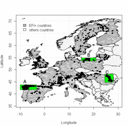
The initial database contains 14221 sites corresponding to 29509 sampling occasions distributed in 15 countries: Austria, Switzerland, Germany, Spain, Finland, France, Hungary, Italy, Lithuania, Netherlands, Poland, Portugal, Romania and Sweden (see Table 1 and Figure 1). More complete information on national dataset1 and descriptions of sampling methods, type of fish data, environmental and pressures variables2 are described in greater details in the previous reports. Fish assemblage described in our working table (N=9948, Table 1 and Figure 1) contains 161 species and 1.938.339 individuals that corresponds to about 43.8 (+/- 11.5) species by country.
Figure 1. Localisation of the sites contained in the three datasets (N=9948): The green (N=533), red (N=2526) and black (N=7244) points correspond to the calibration, slightly disturbed and disturbed datasets, respectively. The light and dark grey polygons identify the countries included in the EFI+ project (see for
more details, http://efi-plus.boku.ac.at/ ).
1 EFI+ 0044096 Deliverable 3_4 New metrics development:
http://efi-plus.boku.ac.at/downloads/EFI+%200044096%20Deliverable%20D3_4.pdf
2 EFI+ 0044096 Deliverable D1_1-1_3 Lists and descriptions of sampling methods, type of fish data,
environmental variables and pressure variables:
Figure 2. Description of the dataset selection process.
The selection procedure to obtain working tables is described in the Figure 2. In a first step, we selected only one sampling occasion by site with a random procedure to limit the potential effect of the temporal autocorrelation (e.g. Pinheiro & Bates 2000, Legendre et al. 2002, Schabenberger & Gotway 2005, Dormann et al. 2007). The exclusion of sites with high rate of missing values provides a new table composed by 10086 sites and 10086 sampling occasions (Figure 1). This simplifies the manipulation and the organisation of the data. In a second step, we keep only sites with complete information on the river typology (Melcher et al. 2007). Finally, our working table includes 9948 sites: 2526 slightly disturbed sites (SID) and 7244 disturbed sites. The calibration dataset (CD) are directly issued of slightly disturbed sites.
Information on EFT typology? One date by site* Initial database: 14221 sites 29509 sampling occasion Intermediatetable: 10086 sites 10086 sampling occasion Final table: 9948 sites 9948 sampling occasion
Slightly disturbed sites (n=2526) Trout zone: 1731 samples Cyprinid zone: 795 samples
Others sites (n=7422) Trout zone: 3188 samples Cyprinid zone: 4234 samples
Training dataset (n=533) Trout zone: 348 samples Cyprinid zone: 180 samples
And 5 additional sites***
Model Computation
Test dataset
Information on the 7 selected Pressures?
Slightly disturbed sites (n=1291) Trout zone: 779 samples Cyprinid zone: 512 samples
Disturbed sites (n=2910) Trout zone: 1033 samples Cyprinid zone: 1877 samples
Pressure Response Analyses
* Random selection of one date by site and samples with high rate of missing data are excluded
** One site by segment and random subsampling selection for sites localized to Asturias and Galicia (ES), North of Poland (PL) and Romania (RO) *** we add five additional site to increase calibration datastet size.
Subsampling, one site by segment** and Captures > 50 Information on EFT typology? One date by site* Initial database: 14221 sites 29509 sampling occasion Intermediatetable: 10086 sites 10086 sampling occasion Final table: 9948 sites 9948 sampling occasion
Slightly disturbed sites (n=2526) Trout zone: 1731 samples Cyprinid zone: 795 samples
Others sites (n=7422) Trout zone: 3188 samples Cyprinid zone: 4234 samples
Training dataset (n=533) Trout zone: 348 samples Cyprinid zone: 180 samples
And 5 additional sites***
Model Computation
Test dataset
Information on the 7 selected Pressures?
Slightly disturbed sites (n=1291) Trout zone: 779 samples Cyprinid zone: 512 samples
Disturbed sites (n=2910) Trout zone: 1033 samples Cyprinid zone: 1877 samples
Pressure Response Analyses
* Random selection of one date by site and samples with high rate of missing data are excluded
** One site by segment and random subsampling selection for sites localized to Asturias and Galicia (ES), North of Poland (PL) and Romania (RO) *** we add five additional site to increase calibration datastet size.
Subsampling, one site by segment** and Captures > 50 One date by site* Initial database: 14221 sites 29509 sampling occasion Intermediatetable: 10086 sites 10086 sampling occasion Final table: 9948 sites 9948 sampling occasion
Slightly disturbed sites (n=2526) Trout zone: 1731 samples Cyprinid zone: 795 samples
Others sites (n=7422) Trout zone: 3188 samples Cyprinid zone: 4234 samples
Training dataset (n=533) Trout zone: 348 samples Cyprinid zone: 180 samples
And 5 additional sites***
Model Computation
Test dataset
Information on the 7 selected Pressures?
Slightly disturbed sites (n=1291) Trout zone: 779 samples Cyprinid zone: 512 samples
Disturbed sites (n=2910) Trout zone: 1033 samples Cyprinid zone: 1877 samples
Pressure Response Analyses
* Random selection of one date by site and samples with high rate of missing data are excluded
** One site by segment and random subsampling selection for sites localized to Asturias and Galicia (ES), North of Poland (PL) and Romania (RO) *** we add five additional site to increase calibration datastet size.
Subsampling, one site by segment**
and Captures > 50
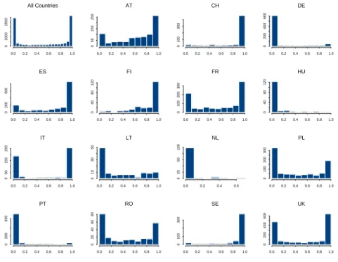
Table 1. Distribution of the sites by country in initial database, final table, slightly disturbed sites (definition given in the next section) and calibration datasets (definition given in the next section).
Country Initial database (N=14221) final dataset
(N=9948) SID (N=2526) CD (N=533) AT 938 840 172 33 CH 717 601 48 26 DE 803 760 33 5 ES 4239 1659 901 97 FI 530 220 137 13 FR 1145 971 185 84 HU 193 146 36 2 IT 652 498 152 33 LT 115 109 54 30 NL 182 105 0 0 PL 919 866 208 53 PT 923 866 8 0 RO 263 239 178 60 SE 615 504 179 56 UK 1987 1564 235 41
2.1.2 Description of the calibration (CD) dataset and description of the slightly disturbed dataset (SID)
The calibration and slightly disturbed datasets are characterized by low level of pressure (Figure 3). The first dataset is used for metric modelling and the second is used to explore and test the responses of metrics in the « quasi » absence of pressure. In contrast to calibration dataset, SID includes between ecoregions sites from all countries and ecoregions (Table 1 and Table 2). In addition, SID, after omitting CD sites can be used as a « quasi » independent validation dataset.
Table 2. Description of calibration dataset (Missing Data were accepted for the variables Acidification and Toxic). The slightly disturbed sites (SID) are selected only by the pressure variables ().
Pressure Variable Selection criteria
Barriers.river.segment.down No or Partial Impoundment No Hydropeaking No Water.abstraction No or Weak Channelisation No or Intermediate Cross.sec No Colinear.connected.reservoir No Toxic.substances No or Intermediate Acidification No Water.quality.index inferior to 3
Table 3. Supplementary criteria for the selection of calibration sites.
Variables type Variables Selection criteria
Effects Hydro.mod No Velocity.increase No Sedimentation No or Weak Instream.habitat No or Intermediate Embankment No or Local Riparian.vegetation No or Slight Temperature.impact No
Water quality Eutrophication No or Low
Organic.pollution No or Weak
Organic.siltation No
Other criteria based on indices Water.alteration No or Medium
Habitat.index No or Slight
Exclusion of Specific sites Water.source.type exclusion of sites characte
by Groundwater water so type
Flow.regime only permanent river
Spatial dependence limitation only one fishing occasio
segment
Sampling constraints captures superior or equal to 50 fish
farea superior or equal to 100 m
month between July and Nove
(included)
The slightly disturbed sites present no or slight degree of perturbation for impoundment, hydropeaking, water abstraction, channelization, cross section, water quality, toxic substances, acidification and collinear connected reservoir. The high rate of missing values is an important limitation in the site selection. As results, to reduce the impact of these ones on the sample size of calibration and slightly disturbed datasets, we accept their presence in two cases: acidification and presence of toxic substance. Then we postulates that the experimenter knows if these two pressures are present and that missing values correspond to no impact.
Calibration sites are included in the SID, but we extend the selection process to the effects of pressure (i.e. modification of the hydrological regime). We only select sites characterised by no (or very few) effects such as embankment, sedimentation, organic pollution or eutrophication (Table 3). We integrate two supplementary indices in the selection process which describe habitat degradation and water alteration. The first, called “Habitat.index”, is based on the aggregation of the value of the three following pressure descriptors: Instream.habitat, Riparian.vegetation and Embankment. The second, called “Water.alteration”, is based on the aggregation of the value of the three following pressure descriptors: Eutrophication, Organic pollution and Organic pollution. More details on these two indices are available in the annex.
Figure 3. Representation of slightly disturbed sites and the three subsampling area (green rectangle): A: Asturias and Galicia (ES); B: North of Poland (PL); C: Romania (RO). The light and dark grey polygons
identify the countries included in the EFI+ project (see for more details, http://efi-plus.boku.ac.at/ ).
To complete the selection of CD, supplementary criterion based on the quality of the sampling is considered to reduce the potential effect of the sampling effort on the estimation of the metric: we only conserve site with caught fish number superior to 50 individual (Table 3). The integration of a constraint on sampling effort is an essential point, because it’s clear that if the number of individuals is too small, estimations of the richness and a metrics are biased (Magurran 1988, Hughes et al. 2002, Reynolds et al. 2003, Hughes et al. 2007).
The last selection constraints concern the spatial organisation of the site at local and large scale. To limit the potential effect of spatial autocorrelation, we excluded the neighboring sites in conserving only one site by segment3 and we use a subsampling procedure for reducing the over-
representativeness of calibration sites located to North of Poland, Romania and to North of Spain (e.g. Galicia and Asturias, Figure 3). The high sites concentration in these three regions could excessively bias the estimation of model parameters and reduced the extrapolation capacity of our models.
After this all operations, we obtained 533 calibration sites to model the metrics. Sample size is appreciably reduced and we only conserve 5.3% of the initial dataset. However, as written previously, a strict selection of the calibration site is crucial to obtain an unbiased calibration dataset and unbiased models.


![[DOC] Cours Merise : le MCT avec exercices d’application | Cours merise](data:image/gif;base64,R0lGODlhAQABAIAAAP///wAAACH5BAEAAAAALAAAAAABAAEAAAICRAEAOw==)