Dynamic sensor tasking in heterogeneous, mobile sensor networks

Dynamic Sensor Tasking in Heterogeneous,

Mobile

Sensor N etwor ks

by

Peter Jones

Submitted

to the Departlllent

of Electrical

Engineering

and CC)lllputcr

Science

in partial

fulfilhllent

of the requirenlents

for the degree of

l\/laster of Science

at the

MASSACHUSETTS

INS1'ITUTE

OF 1'ECI-INOLOGY

l\;J

ay

2005

@

Massachusetts

Institute

of 1'echnology

2005.

All

rights reserved.

~I

~--IJVr~

Author

/

~

(/~

.

Department

of Electrical

Engineering

and COlllputer

Science

l\/Iay 6, 2005

Certified

by ....

Sanjoy

l\/litter

Professor

'Thesis Supervisor

Accepted

by

.(._

';..

'>~':'L'" ~~;.. \:.. "

-./..-'.. : ..

C

.

Arthur

C'.

Snlith

Chairnlan,

Departlnent

COlllrnittee

on Graduate

Students

BARKER

MASSACHUSETTS INSOF TECHNO\...OGY E

Dynamic

Sensor Tasking in Heterogeneous,

Mobile Sensor

Networks

by

Peter .Jones

Sublllitted to the DepartIllent of Electrical Engincering and C0111putcr Sciencc on l\IIay 6, 2005, in partial flllfilh11cnt of the

requirelllCnts for the d(~gree of rvIaster of Science

Abstract

"Nlodern sensor environnlents often attelllpt to ('()ll1hine several sensors into a single sensor network. The nodes of this network are generally heterogenous and llWYvary with respect to sensor cOluplexity, sensor operational llHHles, power costs and other salient features. Optilllization in this enVirOll1lH~ntrequires considering all possible sensor lllodalities and cOlubinations. Additionally, in nlany cases there 111(1)'be a tillle critical objective, requiring sensor plans to be developed and refined in real-tillle. This research will exalnine and expand on previous work in 11l1llti-sensor dyncu11ic schedul-ing, focusing on the issue of near optilllal sensor-scheduling for real-tinle detection ill highly heterogeneous networks.

First, the issue of 11linil1111111tinle inference is fOrIllulated as a constrained optillliza-tion probleln. The principles of dynaillic progral11111ingare applied to the problclll.

A

network lllodel is adopted in which a single "leader" noele nlakes a sensor llleaSUre-11lent. After the 111eaSUreIuentis lllade, the leader node chooses a successor (or chooses to retain network leadership). This lllodel leads to an index rule for leader/action selection under which the leader is the sensor node with lllaxillHlll1 expected rate of infonnation acquisition. In effect, the sensor and lllodality with the lllaxillllllll ratio of expected entropic decrease to nleasurelllent tillle is shown to he an optilllal choice for leader.

The 1110del is then generalized to include networks \vith sirllllltal1eously active sensors. In this case the corresponding optilllization proble111becoilles prohibitively difficult to solve, and so a gallle theoretic approach is adopted in order to balance the preferences of the several sensors in the network. A novel algoritlllll for Illlllti-player coordination is developed that uses iterative partial utility revelation to achieve bounded Pareto inefficiency of the solution.

Thesis Supervisor: Sanjoy ~litter Title: Professor

Acknowledgments

The author would like to acknowledge the following individuals without whose

C011-tributions this thesis would not exist:

Professor Sanjoy l\Htter for advice, suggestions, readings and encollrageIllent Dr. Ali Yegulalp for his service as Staff Illcntor and liason with Lincoln Laboratory The Lincoln Scholars ConlIllittee and Director1

s Office for supporting the research financially as well as through regular feedback and suggestions

Dr. Ed Baranoski for suggesting the probleIll of cooperative sensing in tlw first place

Jason Williauls for suggestions, discussions and frequent help with details

Above all IllY wife who helped when she didn't want to, encouraged wlwn I was frustrated, listened when she\1 heard it all before and cared when I needed it tlw rllost.

Contents

1 Introduction 15

1.1 Sensor Networks .

1.1.1 General Sensor Network Issnes .

is

lG

1.1.2 Exalllples of Sensor Networks 1.2 Scheduling in Sensor Networks ....

1.2.1 Static and DynaInic S('hedlllin~

1.2.2 Schcduling in Detenllinistic SYStClllS 1.2.3 Scheduling in Stochastic SystCIllS 1.3 Proposed l\llethoclology

1.3.1 Scenario ....

1.3.2 lvleasures of Infonnation 1.3.3 l'dininllllll Tillle Fonnulation

1.3.4 Approxilllatc Dynalllic Prograllll11ing 1.4 Silnulated Experinlents ...

1.4.1 Silllulated Environlllcnt 1.4.2 Sill1ulated Sensors.

1.5 Related vVork .

1.5.1 Scheduling in a Sensor Network

1.5.2 Scnsor Nctwork Resource ~lanagelllent 1.5.3 General Optilllization . 1.6 Contributions .... 1.7 Thesis Organization. lG 18 18 19 20 21 21 21 22 24

25

25

26 26 26 27 29

2 Dynamic Problem Formulation

2.2 Optilllal Fonnulations of Inference Problenls 2.2.1 Objectives and Constraints.

2.2.2 Actions in Sensor Networks 2.1 Sensor Network rvIodel ....

31 31 33

34

36 2.3 NIininullll Tillle Equation .

2.3.1 Dynalllic Progranl Fonllulation

2.4 Solution to the l'vlininllllll TinlC FOrInulation

2.4.1 Optilnal Actions in DeterIninistic Networks 2.4.2 Optilllal Actions in Stochastic Nctworks

2.5 Conclusiolls .

3 Cooperation for Tinle OptiInal Inference

3.1 Introduction .

3.1.1 Planning Paradignls 3.1.2 A Note on TerIninology .

3.2 Extending Nlaxinllllll IAR to l\lulti-Scnsor Deploynlcnts . 3.2.1 l'vlonolithic Joint DeploYlllCllts . 3.2.2 A Gallle Theoretic Approach to l\IaxilIlizing Group IAR 3.2.3 Uncoordinated Solution l\;lethods

3.2.4 Coordinated Solutions . 3.3 Increasing Sensor Utility through Side Paynlents

3.3.1 T\vo- Player 1 Two-Action GaIlle . 3.3.2 T\vo-Player1 l\Iulti-Action GaInes

3.3.3 l\llulti- Player1 j\1ulti- Action GaIlles

3.4 A Silnple Denlonstration of Side Paynlents 3.4.1 Solution Perfonllance ...

3.5 Linlitations and Possible Extensions . 4 Simulated Implementation and Results

4.1 SiIllulatioll Setup . 49 51

54

5G

58

GO

66 67 72

75

78

81 81

4.2 Single Sensor Silllulation .... 4.2.1 Silllulatecl Environlllcnt 4.2.2 Sensor l\Ioclcl .

4.3

rvr

ultisensor Silllulation

4.3.1 HOlllogcncous 1\1ulti-Scnsor Experillll'nt

4.3.2 Heterogcncous l\1ulti-Scnsor Expcrilllcnt

4.4 Results Sunllllary . 5 Conel usion 5.1 SUllullary 5.2 Future Work. 81

82

82

87

88

DO

D1

List of Figures

2-1 Sensor network in a naval battlefield scenario (courtesy of [2G))

2-2 Dynalnic decision flow .

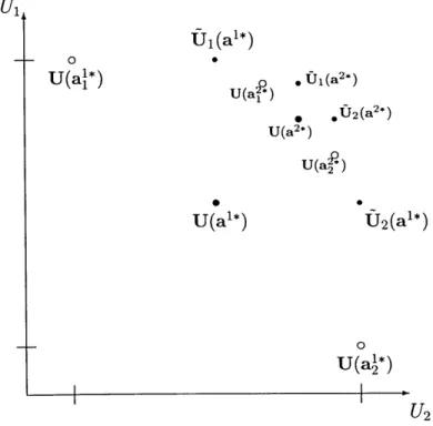
3-1 (a) Loose bound on Pareto suboptilllality of the negotia ted solution (b) Tighter bound on Pareto suboptinlality whell the negotiated solution

is unclolllinated .

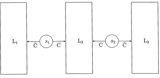
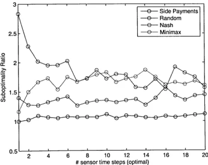
3-2 Two-player, nlulti-action utility space 3-3 Silnple cooperative sensor situatioll 3-4 Suhoptilnalities for four algoritllllls 4-1 Exanlple of a sinnllated battlefield. 4-2 Sanlple entropy trajectories vs. tilllC

4-3 Relative Perfoflllance Loss as a FUllction of 7; 4-4 Trial-by-trial difference in cleploYlnent tilllCS . 4-5 Algoritlull effectiveness uncleI' increasing SNR

G'r:_.) 72

7G

82

84

8G

87

89

List of Tables

3.1 Cannonical payoff lllatrix .

3.2 Silnple ganIc payoff lllatrix

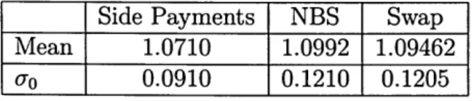
3.3 Statistical conlparisoll of solution lllethods

3.4 Statistical cOlllparison of coordinated solution lllCthods

4.1 Statistics for 100 runs of single sensor, single lllode silllllia tioll

4.2 Statistics fOf50 rUllS of singlc scnsor, llllIliplc IllOdc sillllIlation

4.3 Statistics for 300 fUllS of hOIllogcncous, llllIlti-scnsof sillllllation . 4.4 Statistics fOf 100 fUllS of hcterogcncous, llluiti-scnsor sillllllation

GO

73

77

78 87 88

Dl

Chapter

1

Introduction

1.1

Sensor Networks

A sensor nctwork is any c()lnbination of two or nlorc sensors capablc of intcractin~ eithcr directly through scnsor-to-scnsor COIlllllllnication or indircctly through ccntral-ized infonnation sharing. Scnsor nctworks COl11ein nlany configurations and levels of cOlllplexity. They Inay consist of a handful of individual scnsors or sevcral thousand

(or lllore). They Inay be hOlnogcncous (popula tcd by idcntical sensors) or hctcro~(~-nous (populated by two or lllore types of sensors). Thc sensors thclllsclves can range froln the silnple, such as passive, singlc-lllode nlagnetol11eters to the cxtrclllcly ('0111-plex, such as airborne synthetic aperture radars (SAR,s) capable of operating in a variety of lllodes and the ability to direct sensing to specific area.'" throngh bealll forming and radar steering.

But regardless of size, configuratioll, heterogeneity and sensor cOlnplexity, all sen-sor networks face silnilar issnes. All sensen-sor networks are inlplenlented with the goal of observing the environlnent, taking IneasurClllcnts and infcring sonle \vorlcl state froin this infonnation. Raw data collected by the sensor nodes lllust SOIllChowbe culled and collated to fOrIn a unified estilnate of the world state. A problcnl of con-verting ra\v data into infonnation is conllnonly called an inference problem. SonIC exanlples of inference problenls in sensor networks include the detection, tracking and identification of targets of interest.

1.1.1

General

Sensor Network

Issues

No network has infinite resources. All networks. whether silllple or conlplex. nlust re-alize a resource lnanagenlent strategy in order to acc()lllplish the sensinp; p;oals such as target detection, tracking and indentification. I3esides lilllitations due to the nUlnber of sensors available within the network, other constraints nlaY include tinH~, eIH~rp;y, lnaterial cost, or conllnunication. These constraints will he collectively ternl<'d costs. Achieving sensing goals while lninilllizing costs requires careful planning and resource lnanagelnent.

Resource lnanagenlent can be significantly conlplicated by network heterop;el}(\-ity. If the sensor network is hOlllogcneolls, nH\Cl.ninp;all sensors have essentially tlw saIne capabilities, sensor InanagenlCllt beconws arhitrary to a certain extent. In ho-lllogeneous networks, the network ability to achieve its goal is invariant lIndeI' the particular sensor chosen for each sensing task. In IH'tcrogcncous networks, howcver, each sensor has unique abilities and lilllitations. This diversity disrupts the the net-work assignlnent invariance. The lltllllber of possible cOlllbinations for scheduling can quickly overwhehn the planning capabilities.

1.1.2

Examples

of Sensor Networks

Sensor networks are becolning increasingly popular in lnilitary and industrial applica-tions. Listed belo\v are several exanlples of lnodern sensor networks, all drcllnatically different in structure, but essentially silnilar in the purpose of trying to accurately detennine the current state of an envirOlllnent of interest.

Example 1: Walrnart recently announced that it will encourage all suppliers to attatch RFID tags to their products. RFIDs are very silnple sensors with no power source. They use the energy of a satellite radio wave to acconlplish their task, which is to geolocate themselves. This is an exanlple of a hOlnogeneous sensor network, where all sensors are essentially identical. The resources involved include the tilne it takes a tag to respond to queries about its position as well as the energy cost of translnitting the position. In this network, the inference problenl is to deteflnine where an itenl is

at any given tinle. Using the RFID sensor network to solve this probl(,111 will result in greater efficiency in vVahnart's supply chain, and lower overall product costs for its conSUlners.

Exarnple 2: The Advanced Network Technologit's division of the National Institue of Standards and Technology has ongoing research regarding the use of se11sor net-\vorks for search and rescue operations. The networks would function in (\nVirOnnlents unsuitable to lnllnans, enabling search and rescue workers to penetrate hazardous en-vironlnents and locate rescue candidates. Such a systelll was deployed by a t(\anl froln the University of South Florida following the collapse of the \\Torld Trade C(\n-ter buildings. A wirelessly connected group of llloblie robots, each with several sensors attatched, \vere used in the search the collapsed buildings for trapped victi111s. In this case, the networks was slnall scale (5-10 robots) and lllostly hOlllogeneous (all robots \vere silnilarly constructed and had silllilar sensing abilities). The goal of identify-ing rescue candidates is tillle critical, since the longer the delay the less successful eventual rescue will be. Therefore the prilllary cost to the network was tillle.

Example 3: The scenario of interest for this thesis, which will be described in 1110re depth in Section 1.3.1, is that of using sensor networks for battlefield awareness. In this case, the set of sensors is heterogeneous and range froln silllple acoustic sensors to highly cOlnplicated, satellite-based radars. Sensors in the network differ in their level of lnobility, their available lnodes of operation, and their ability to detect targets of interest. The inference problelns in this network include target localization, tracking, and identification. The costs in this network are varied, including c0111111unication, fuel expenditure, sensor detection and interference by the enenlY and l11orc. However, as with the search and rescue exalllple, in lnany cases the prilllary concern is one of tinle, in that targets lnust be isolated and identified as soon as possible.

The above exalnples represent a slnall sall1pling of interesting sensor networks. For a more conlplete discussion of areas in which sensor networks are being utilized, see

[13].

\\Thile the inference problell1s solved by sensor networks can vary as greatly as the networks thell1selves, the fundalllental issnes of resonrce lnanagclnent and achieving goals under cost constraints are relevant to all real sensor networks.

1.2

Scheduling in Sensor Networks

Sensor net\vorks generally nlust develop a sensor plan or schedule in order to achieve sensing goals such as target detection, tracking and identification. The sensor plan detennines \vhich resources should be used, in what order and for how long. The sensor plan will directly detennine how n1\1ch tinlC, energy and nlat<~rial cost the net\vork Inust use in order to achieve the sensing goals. The purpose of the scheduler is to create a sensor plan which willlninilnize the cost required to solve tll<' inference problelll. This can be represented by the equation

p*

=

arg Inin C (p)

pEP

(1.1)

where C(p) is the cost (in resources) of executing plan p and P is the set of all plans that result in the solution of the inference probleln.

A

plan p consists of an onlered set of actions, 0,1...aN. In the case of sensor networks, the actions are queries or deploynlents of specific sensors. Each action Inay involve querying or deploying any subset of the sensor network.

Despite the Silllplicity of the optilnization equation, tIle job of the sclleduler is cOlnplicated by several issues, including the dynalnics of the network, tIle stocha~tic nature of sensor Ineasurelnents, and the uncertainty in calculations of cost, current knowledge state or both.

1.2.1

Static and Dynamic Scheduling

Algoritluns for scheduling fall into two broad cla.sses: static (open-loop) and dynalnic (closed-loop). Static scheduling is Inuch silnpler, but is lilnited in applicability because it cannot react to unexpected changes to the systeln. Dynalnic scheduling, while significantly Inore cOlnplicated, is generally Inore robust due to its ability to adapt during the course of plan execution.

In open-loop scheduling, the scheduler detennines a cOlnplete plan pnor to the beginning of the plan execution. The plan cannot be 1110clifiedonce execution ha.s

be-gun. Open-loop scheduling has the benefit of silnplicity and case, and in detenninistic systen1s can guarantee achievenlCnt of the systenl goal. However, static progralllllling suffers fron1 an inability to react to infonnation obtained during the execution stage. Additionally, in stochastic systellls open-loop scheduling generally cannot guarantee the eventual achieveluent of the systelll goal, since the results of actions are inhercntly unpredictable.

Closed-loop, or dynaluic, scheduling involves interleaving decisions with actions, enabling the systell1 to lllake scheduling decisions based Oll all infonnation obtaincd up to the current till1e. In this case, the scheduler can rcact to infonnation obtained during plan execution in order to ensure that appropriate actions are taken at each new step of execution.

Dynaluic scheduling depends on the principle of optillw.lity, first identified by Belhnan [3]. This principle states that if a path frolll a start state to a goal state is optilual, then the subpath frOlll any intennediate stat(~ to the goal state will be optilual for the subproblelll of llloving frolll the intenncdiate state to the goal. Using this principle we can 1110dify1.1 to read

a*

1

a*

N

argllllllnEA, (C1(a)

+

C}(P7+1)) arg IIlillnE,'\JVC1(a)

(1.2)

and

pT

=

{aj}f=i'

C(a)

is COllllllonly refcrcd to as the ilnll1ediate cost and C}(P7+1) as the cost-to-go. Progralns fonl1ulated as 1.2 arc called dyncunic prograIns and the lnethod of solving thelu is called dynaluic progralllluing.

1.2.2

Scheduling in Deterministic

Systems

It can be shown (e.g. [5]) that in detenuinistic systelns the optill1al open-loop schedule is equivalent to the optinlal closed-loop schedule. In a degenerate sensor network \vhere all costs are known a priori ancl sensor 11leasurcnlcnts have no ranclolIl clclllCnt, there is no need for a scheduler to be reactive, since no unexpected infonnation will ever occur.

Consider for instance a network populated by sensors, 8{1:M}' Suppose the

infer-ence problenl for the network is to achieve a certain level L of confidinfer-ence under son1e Ineasure. Each sensor contributes a detenllinistic "alllounf~ of confidence

Ii

at a cost Ci and the total confidence is

L~~

11(11 and the total cost is

L;:

1('(II' This prohlenl

can be ll1apped to a generalized knapsack problelll \vhich is exactly solvable prior to the beginning of execution (although not in polynonlial til11e). \Ve will return to this degenerate fonnulation in Section 2.4.1.

1.2.3

Scheduling

in Stochastic

SystenlS

In the case of stochastic systel11s, the optilnal open-loop schedule will not generally be equivalent to the optilllal closed-loop schedule. In stochastic systen1s, total cost can be inlproved by reacting to infonnation gained during plan execution. Fron1 the above exaluple, if the "aI110unt" of confidence frOI11sensor iis non-detenllinistic, the shortest path probleln becolnes a stochastic shortest path problel11. Any static plan in this systeln would suffer fronl an inability to react to an unexpected

it.

Say, for instance that in creating the static plan, the planner anticipated that after the first

k Ineasurenlents the total level of confidence

L~~

1 Ii would be equal to L and the task would be cOlllplete. The optilllal plan \vould not schedule any nlore actions, since the goal would have been achieved and 1110rcactions \vonld oIlly incrcw..;c the total cost (assullling Ci

>

0 Vi). If, however, the actnal level after k n1easurClncnts is

L

<

L, a scenario which Inay occur due to the stochastic nature of Ii, the optilllal static plan cannot schedule 1110reInea..'3Ure111ents,and the sensing goal will therefore not be achieved.

Scheduling in stochastic systel11s can be extelllcly cOlllplicated and COlllputation-ally intensive. The fonllalization of DP (dynall1ic progra1111l1ing)requires the consid-eration of all possible action sequences that result in achieven1ent of the goal state. This can be illlproved sOlllewhat by advanced techniques, but the inherent cOll1plexity is invariant to such techniques. This is particularly problelnatic for prograllls where the set of possible actions is large. For the sensor lletwork~ the nlllnber of possihle actions at each decision stage is cOlnbinatorial in the nUlllber of sensors~ resulting in

a very large action set. In COlllplicated stochastic networks lllethods of approxilllat-ing the optirnal solution are of great irllportance. SOlne approxilllate lllethods are suggested in Section 1.3.4.

1.3

Proposed Methodology

1.3.1

Scenario

One interesting application of sensor networks is in the area of battlefield aware}}('ss. Battlefield awareness is the ability of a lnilitary unit to accurately lnodcl the curn~nt field of engageInent, especially as regards the detection1 tracking alld identificatioll of

targets of interest. This awareness is central to the success of lllilitary call1paigns. The proliferation of possible sensors for use in battlefield awarencss has dralllat-ically increased the ability of lnilitary ullits to accuratdy lllodel the field of engage-lnent. The challenge is to detennine froln alllong all the possible sensor deploYll}(~ntsl which deploynlent ,viII achieve awareness goals while }ninilnizing total SYStclll costs. To better define this problenl we llluSt define the "awareness goals" of the Systclll a~ well as the systern costs.

1.3.2

Measures

of Information

One of the central problenls of infornlation theory is how to lneasnre the infonnation content of a rnodel. Exalnples of this problelll include lneasuring how accurntely a quantized number represets a continuous nurnber or how well an estilnated probability function represents a true probability function. The latter exalllple is relevant to the question of rneasuring the infonnation in a sensor network tasked with target detection. In this case, if we let X be the set of possible target locations, the true probability function is { I if.TE)( p(x)

=

0 otherwise (1.3 )

Knowledge of this true state is obtained through a series of observations \vhich are aggregated into a conditional probability function ]J(:rlz). where z is the set of ob-servations. Infonnation theoretic nlethods, including Shannon entropy and relative entropy, can be applied to p( ~r

I

z) to nlcasure how well p(.r

I

z) a pproxinla tes the true probability function in Equation 1.3.

Let z

=

{Zd~l

be the set of collected seIlsor llH1ClSllrellH1Ilts.TheIl, uIlder the ClS-slunption that sensor IlleaSUrenlellts are independent of OIl<'ClIlotll<'r. we can fOrIllltlate a Bayesian estilnate of

p(

~r) as

N

p(:rlz)

=

n * ]Jo(;l:) IIpi(zil:r) i= ]

(1.4)

\vhere po(x) is the a priori probability that :r E ~Y, N is the nUlllbcr of sellsor IneasureIllents, Pi (Zi I:[) is the conditional probability of sensor IlleaSUrenl<'nt Zi g;lven x E X and ex is a scaling constant.

There are several possible l11easurcs of the inforIllation contained in ]J(:r

I

z).

Per-haps the Inost well known is the Shannon entropy, due to Claude Shannon, the father of inforInation theory. Shannon postulated that the inforllw tion in p(:r Iz) is related to the uncertainty in

p(xlz).

He then showed that the uncertainty of p(:rlz) can be 111easured using the negative of the BoltzInann entropy, or

tl(p(xlz))

= -

J

p(.rlz)log(p(xlz))d:r

Thus, one \vay of fonnulating the inference probleIll is to declare it solved once the entropy is driven below a threshold, i.e. IL(p(xlz)) :::; ,.

1.3.3

Minimum

Time Formulation

In the case of battlefield awareness, there are several possible cost fOrInulations for a particular sensor plan. In this thesis we will focus on the tilne costs of the systeln.

Thus, the optilnization equation 1.1 can be written

p* = arg Iuin

E[

f,(p)]

pEP

(1.5)

The expectation E[t(p)] is necessary when the exact length of tinH' bd,w('('n the deploYlnent of a sensor and the availability of its nH'aSUrenH'llt is unc<'rtain. For nlost sensors, at the tinle of deploYInent only an expected tiine or range of tillH'S until nleasurenlents are available is known.

Additional uncertainty conICSfroin the stochast.ic nature of the scnsors UH'nlse}vcs. Without loss of generality we can restrict our attention to sensors for which it is not possible to know beforehand what a particular sensor llH'(lSUrenH'nt.will be. (Infor-InaUy, if a sensor's IneaSnrenlent were predet.enllincd and it was included in a sensor plan, the sensor plan could be iIllprovcd by renloving the planncd nH'a.surclllcnt, sincc the sensor Ineasurelllent cannot decrease systelll uncertainty and can only increase the total tinle of plan execution).

Since the systelll is stochastic dne to uncertainties both in the cost function and in the future knowledge states (i.e. sensor IneasurClnents), a dYllaIllic scheduler will be able to achiever higher levels of optilllality than a static scheduler (see Section 1.2). We can reformulate the tiIne Ininiinization probicill in the forlll of Equation 1.2

(1.6)

and

p;

=

{aj}j:i

and JV is the total nUlllber of actions in the sensor plan. This states that the optilnal action at any given tilne is the one that lniniluizcs the tinlC it takes to accolnplish the action plus the expected tilllC it will take to achieve the systelll goal once the action has been taken.

1.3.4

Approximate

Dynamic

Programming

In solving for the optilnal action

a;,

two quantities Blllst be calculated: the inllne-diate cost and the expected cost-to-go. Solving for the optilnal cost-to-go involves

constructing an optiInal plan froIn the tinle thc current action cOIllpletes until the systeIll goal is Inet. This subproblcnl can hcconlc extrcnldy conlplicated. Even in sinlple scenarios it can be cOInputationally prohibitive to sol\'(~ this probleIll exactly. Frequently, approxiInatc Inethods IllllSt be introduced in order to decH'ase the conl-plexity of the problenl.

The siIllplest approxiIllatc lllCthod is to aSSUIlH' the cost-to-go is negligbl('. This leads to algoritluns which l11iniIllize inlIllCdiate costs with llO thought for future heIl-efit. These algoritluns are generally called greedy algoritllllls. In tl}(~case of tll<' fonnulation we are considering, the greedy algoritlllll would result in a plan ac('ord-ing to the equation

iii

=

arg Illin E(l(a)]

(IEA,

However, if we aSSUI11ethe null action (i.c. 110se11sors deplo.yecl) is always all option, this greedy fonnulation will result in a plan in which no action is ever taken! Although other greedy fonnulations can 11litigate this effect, they all suffer fronl tlw problelll of neglecting the contribution of future states to the total cost of a sensor plan.

Another possibility is to approxilllate

E[t.(pn]

by SOIIlCeasily COIllputahle heuristic function

H

(Pi). Heuristic nlethods can significantly reduce the (,olllplexity of the scn-SOl'planning problenl itself, but introduce the problclll of choosing which heuristic to use. In general, the closer a heuristic COl11esto the ideal cost-to-go the better tl}(' re-sulting algoritlun perfonns. SinuIlation based Illethods and ncuro-dYllclll1ic progrmn-nling are two heuristic nlethods that have proven effective at finding approxinHltly optinlal solutions \vhile lilniting cOlnplltational cOIllplexity.

1.4

Simulated Experiments

ExperiInents were perfonned to verify the theoretical developIllents of this thesis. As stated in Section 1.3.1 the scenario of priInary interest is one of detecting battlefield targets. The eXperiIl1ents were designed to iIllitate features of the battlefield awareness problClll and consist of both siInulated sensors and siInulated environIIlents.

1.4.1

Simulated Environnlellt

The experilnental environnlCnts were intended to 1110dd actual battlefield enVlron-lnents. The siInulated tasks were prilllarily detectioll and discrilliinatioll tasks. al-though other inference problenls could also be tested in the Sa111('enVirOnllH'nts. The envirOlunents consisted of a discrete lllunber of possible target locatiolls. T'argets could exist in any of the locations and could be of sev<,ral tY1><'s. A priori prob-abilities for each target type at each possible location were known by tl1<' s<,nsors. The specifications of the environnlCnts for each sillllllat<,d <,xperillH'llt are giv(~ll ill Chapter 4.

1.4.2

Simulated

Sensors

Sensors \vere sinlulated to have a variety of abilities and lilllitatiolls. Both 1110bilealld stationary, low and high power, single and llluiti-lliodal sensors were used ill the SillIU-lations. The sensor differences resulted in varying abilities regarding resolution, noise suppression, and lneasurelnent tinle and range. The silllulated sensor configuration, including choice of sensing location and lllodality, affected the sensors' probability of false alanns or lnissed detections. This is true for real sensors. For instance, if the Inagnetolneter froln

[10]

is deployed to a locality high in llletallic concentration, the probability of false alann \vill increase draIllatically. Silllilarly, if the airborne, bi-Illodal SAR discussed in

[30]

operates in HRR, lllode over a forest, the probability of nlissed detection \vill be increased due to foliage occlusion. This sensor / environnlent dependence was sinullated by assigning to each cnvirOIlIllent locality and each sensor and 1110deof operation a Signal-to-i\oise ratio (SNR). High SNRs result in better ability to detect targets. The specific sensor nlodel is given in Chapter 4.

1.5

Related Work

1.5.1

Scheduling

in a Sensor Network

A starting point for this t\Iaster's Thesis is ?\Iaurice ehu's doctoral thesis

[10].

In this \vork, Dr. Chu develops an optilnal nwthod for distributed inference in a lar~e scale sensor net\vork. Additionally, he proposes a technique for sub-opti11lal inference when only local knowledge is available, as when only a subset of the network sen-sors report Ineasunnents. This Inay be plaIl1wd (e.~. to linlit power conSU111ption), or unplanned (e.g. sensor failure, network .ia11l1nin~, 11leSSa~eloss). He uses a COlll-binatorial approach to sensor planning, creatin~ a cOlllplete set of sensor plans for all likely sensor readings. He then derives a syste111 of trig~ering events. The nlain purpose of this systeln is to lilnit the aillount of llllJle('(\SSary infoflnat.ion ga tlH'l"('d in the sensor network. Evaluation of these triggers can be dist.ribut.ed aillon~ net.-work nodes, Ininirnizing the tillle necessary for detect.ion. Foundational work for Dr. Chu's method includes [9, 43] where the Infoflllation Driven Sensor (~uery (IDSQ) Inethod for sensor scheduling was derived. IDS(~ ha.s been crit.iqued and expanded upon in [13, 41, 22].

1.5.2

Sensor Network Resource

Management

A central focus of the thesis is how to extend the infoflnation theoretic principles derived in [9, 10] to a situation in which llluitiple sensors can be sillllIltaneously active. In [42] lllany of the issues involved in rllulti-sensor lllallagelllent arc surveyed, including issues related to the optinlal placelllent of sensors within an area of interest, the benefits and constraints of decentralized control, and sensor cooperation.

In addition to inter-sensor Illanageillent, the optinlal choice of 11lOdcfor a single sensor is also relevant to the developnlent. In

[30]

an optilllization involving a single, rllulti-rllodal sensor suite was presented. Additionally the issue of sensor placeillent for 1110bile,active sensors described in (11, 16] can be considered as atteIllpts to optilnize over a continuous lllode of operation (in this case, geographical placenlent) in order to

achieve goals which lnay change with tilllC. The ability to optilllizc over continuous lnodes is essential to planning in nctworks involving active sensors.

1.5.3

General

Optimization

Applicable research not specific to scnsors and sensor networks includes the theory of dynalnic progranllning (cf. [5]) and the closely relatt'd work in l\larkov Decision Processes [12]. The basic theory of dYllaIllic progralllllling extends traditional opti-lnization analysis to a set of problclllS which vary with tin}('. It provides a structure for decision feedback and sequcntial decision analysis. enabling inforInation to l)(' incor-porated in an optiInal nlanncr while it is being gathered. This appli(~s din'ctly to tlH' thesis, in \vhich a sensor plan lnay need to be nHHlificd as new sensor nH'aSnn'lllellt.s are lllade and incorporated into the likelihood functioll.

Dynalllic prograllllning is a powerful tool, but call l)(~COlllputationaly prohibitiv(~ to inlplenlent, particularly in problellls where the state space is large. To address this issue, learning algoritillns have been developed to approxinlate the optilllal so-lutions found through dynalnic prograllllning. NcurodYalllllic progralllllling [G), or "reinforcelllent learning" as it is sOlnctinles known, uses neural network and other approxinlation architectures to adapt dynaIllic progranllning llH'thods to cOInplex environnlents.

Dynanlic progranlllling has becn previously applied to scnsor networks in [:39,

:31].

It has also been used to analyze single sensor InanagcIllent

[7]

as wcll as to general real-time environments

[2].

In addition to dynaIllic prograIlllning, othcr optiIl1ization tcchniques Illay bc CIll-ployed, particularly in optilnizing the cost-to-go sllbprohleIll. These techniques Illay include nonlinear, nlixed-integer, and/or constrained progranlIlling [4, 21].

1.6

Contributions

Previous research in sensor schcduling has focused priInarily on iInproving the quality of inference [9, 13, 39, 10]. \Vhen rcsource costs havc becn considered they have been

linlited to power constunption due to cOlllnHlllication [22, 41]. and have generally been treated as constraints on the set of feasible solutions rather than as elcnlents of the objective. This thesis fOrIllulates the prohlclll as one in which the quality of the inference is the constraint, while the systenl cost is a fund ion of the anloullt of tilne the schedule takes. The prinlary objective is not to achi(l\'(' a hi!!;h quality of inference independent of how long it takes, hut rather to achievc a "good cnough" estinlate as quickly as possible. TilHe nliniIllizatioll is fUlldaIIH'ntally import.ant. In Inany applications, and exalnining this fOrIllulation will (~xpalld tlH' usefulncss of sensor net\vorks in both Inilitary and industrial applications.

Additionally, the InininHllll tillle fOrIlllllation I}(lcessitates a considcration of spnsor interactions. In n1uch of the previous work in spnsor lletworks, it is assuIlH'd that a single "leader" sensor is active at any given tilllC alld all other sensors ill tlH' lld,work are inactive. This assulnption sinlplifies IllllChof the analysis, but in the fOrIllulatioll for this thesis it significantly reduces the optiIllality of tl)(~ solution. It is essential to consider Inethods for sensor schedulillg whcll nllIltiple sensors IlUlYhe active at the sanle tilne. Applying clelnellts of gaIlle theory to this prohlenl of IlllIltiple sensor coordination is an ilnportant contribution of this thesis.

One of the central issues facing the United States Illilitary is the efficient use of 11lultiple sensor platfonns. The past twenty years have seen an unpn'cedentcd nUlnber of sensors developed for Inilitary application. There are sensors in the air, on land, on sea, underwater and even in space. Each sensor has unique capabilities that Inake it nlore valuable in S01l1esituations and less valuable in others. The wealth of sensors available presents two significant problellls: one, how to deal with the copious alnounts of raw data produced (so Inuch that it often overwhehns IHllnan analysts): and two, how to enable efficient sensor cooperation. Since the sensors were developed individually they often suffer frolll what's called stove-pipe sensing, Illcaning it is difficult to use sensors cooperatively.

The principles derived in this thesis, especially the cooperative architecture de-veloped in Chapter 3, address these two problenls. Through increasing the HutollOlny of the sensor network, less data need be analyzed by 11l1l1lans.The architecture also

provides a fraluework in which several sensors can efficiently cooperate in a highly dynaluic and unknown environluent. The contributions of this thl'sis will dirl'ctly and innnediately influence the future devclopnlCnt of intcgratt'd sl'nsing platfonlls for the U.S. luilitary through ongoing research at l\IIT Lincoln Laboratory in the Int('grated Sensing and Decision Support (ISDS) group.

1.7

Thesis Organization

This chapter has served as an iutroduction to SOlllCof the issues involved in s('eduling sensor networks. Specifically, a cHnnollical deU'ction scenario ba.sed on ba ttldield awareness has been presented, an objective of nlinilllizing tin}(~to n~ach an acceptabk state of certainty has been stated, and a lllCthod for accoillplishing the objective ha.s been proposed.

In Chapter 2, sensor network inferellce probleills will be discussed ill gn~ater detail. Then the lnininnuu tillle optiluization fOrIllUlatioll frol11Section 1.:3.:3will he developed and analyzed using lllethods frolu dynalllic progranlllling.

Chapter 3 will discuss the need for coordination in solving ccrtain inference prob-lenls in sensor networks. It will then present a cooperative, distributed Incthod for achieving the optiIual sensor deploYlllCnts derived in Chapter 2.

Chapter 4 will introduce sinl1llations used to verify the algoritlllll proposed in Chapter 3. The silnulation will consist of general classes of environnlcnts and a suite of available sensors. Results froIn the sillullation will he presented along with an analysis of the observed strengths and lilllit at ions of the algorit1lln.

Finally, in Chapter 5 conclusions will he drawn as to the viability of the derived algoritlnn and its possible extension to new dOlnains.

Chapter

2

Dynamic Problem Formulation

2.1

Sensor Network Model

As discussed in Chapter 1, an important use of sensors is in improving battlefield awareness. Sensors currently used in this type of situation are highly varied and in-clude both active and passive, mobile and stationary, single and multi-modal sensors. Figure 2-1 depicts a typical battlefield scenario with a network made up of highly varied sensors.

Each sensor in a network has a set of possible measurements it may receive. For instance, the stationary magenetometer described in [10] measures either a 0 or a 1, depending on whether any magnetic material is detectable in its area of observation. A mobile radar has a different set of possible measurements, based in part on its position, velocity, pulse frequency, dwell time and other operational paramaters [34]. Using such varied assets conjointly is Inade possible if the network is capable of aggregating the various measurements into a single, universally understood model.

Consider sensor Si E S, where S is set of all sensors in the network. Assume Si has a

measurement model consisting of the 2-ple

(Zi,Pi(zlx)),

where

Zi

is a set of possible measurements, and

Pi(zlx)

is the probability of observing measurement

z

E

Zi,

condi-tioned on the true state

x.

Furthermore, assume that for all Si the set of possible true

states is fixed and known and that measurements are conditionally independent given the true state, meaning that Y i,j

Pij(Zl,

Z2!X)

=

Pi(Zllx)

*

pj(z2Ix),

Zl

E

Zi, Z2

E

Zj.

Figure 2-1: Sensor network in a naval battlefield scenario (courtesy of [26])

Under these assumptions the network can rnaintain a global probability function

7r(xlz)

(where

z

=

{Zi}~l)

if each tinle sensor

Si

obtains a new rneasurernent, the global probability function

7r(xlz)

is updated by the sensor to be the optimal poste-rior probability function. For detection problems this would be accornplished by Si

calculating and then broadcasting to the rest of the network the Bayesian update

(2.1)

where ZN+l is the most recent measurement observed by Si.

In

other inference

situ-ations (e.g. tracking, localization, discrimination) other update rules might be used, but the process would be the same. The sensor taking the measurement updates the (global) posterior probability function using its (local) rneasurernent lllodel and the known update rule

f(7r, z,p(zlx)).

In

general, the posterior distribution will be

updated after the Nth measurement by

7r(xl{Z}:;=I)

=

f(7r(xl{z}::::i

1),

ZN,P(ZNlx)).

An inference problem is defined by the 3-pIe

(X, Po (x),

f (.,.,.)).

X is the set of possible decisions, corresponding to the fixed and known true states of the sensor models,

po(x)

is the initial probability of each of the states and

f(.,.,.)

is the update rule. An inference problem is solved by a decision rule

D : [(X,Po(x),

f(.,., .)),

z]1---7

X. Thus, an inference problem is solved when one of the possible states is decided for and the rest are decided against.

2.2

Optimal Formulations of Inference Problems

As stated in Chapter 1, an inference problem is any instance of converting raw data to information. In the case of sensor networks, inference problems include transform-ing a set of RFID tag responses to locations, determining the location of possible victims from search and rescue robots' sensor responses, or localizing, tracking and identifying an enemy target within a battlefield. Inference problems are as diverse as the networks used to solve them, but all inference problems involve the ability to extract information from raw sensor data.

A sensor network's capability to solve inference problems can be formalized as an optimization problem. The most general format of an optimization problem is

x*

=

argminxEx

f(x)

s.t.

g(x)

EG

(2.2)

The function

f(x)

is called the objective function,

g(x)

is called the constraint function or constraint and G is the constraint set. A solution x is called feasible if

g(x)

E G, and the set F =

{x : g(x)

E G} is called the feasible set. A solution

x*

is called optimal if it is feasible and

f (x*) ::; f (x)

V

x

E

F.

In sensor networks, there is some variability in how the objectives and constraints from Equation 2.2 are chosen. This variability results in a variety of optimal for-mulations, each providing unique insight into the operation of the sensor network. Which formulation should be used is dependent on the specific goals and design of

the system.

2.2.1

Objectives and Constraints

As discussed in Section 1.1.1, there are several possible costs due to resource consump-tion in a sensor network, including costs due to communicaconsump-tion, time, and energy. We will refer to these collectively as consumption costs. Additionally, inaccurate solutions to the inference problem (e.g. missed detections, bad localizations, etc.) carry some cost. We will term these quality costs. The objective function and the constraints for Equation 2.2 derive from combining quality and consumption costs. Different categorizations lead to different optimization formulations.

Minimum Consumption Formulation

A sensor network must consume some amount of its resources while solving an in-ference problem, meaning it must use some amount of time, energy, communication and so forth. In the minimum consumption formulation, the objective function is a measure of the resource consumption of a network. The quality costs are incorpo-rated through the constraint function. The goal under this formulation is to consume as little as possible of the network resources under the constraint that the resulting inference problem solution meet some minimum quality requirement. As an example of a minimum consumption formulation, consider the following problem statement: minimize the energy used in a network while guaranteeing a probability of detection no less than,. In this case the objective function is the energy consumed by the network (a consumption cost), the constraint function is the probability of detection

(quality cost) and the constraint set is the set of all solutions with probability of detection greater than or equal to ,.

One of the challenges of using a minimum consumption formulation for systems with diverse consumption costs is in the determination of an objective function that balances the consumption of the various resources. For instance, which solution has lower cost: one that satisfies the constraint in 5 minutes using 1 W of power, or one

that satisfies the constraint in 50 minutes using 1 m W of power? The answer depends inherently on the purpose and design of the network. Aggregating consumption costs into a single objective function can be very challenging.

Maximum Quality Formulation

In this case, the objective is to minimize the quality costs of the solution. Quality of the solution refers to the probability of making a wrong decision. Take for example a localization problem. The inference problem is to determine the location of a target. The objective function might be the expected mean square error of the estimated location from the true location. The objective function is a measure of the quality of the inference problem solution.

In the maximum quality formulation the consumption costs are incorporated through constraint functions. Thus, using the localization example, one constraint might be that total energy expenditure in the network is less than E mW, or that a final estimate is reached in no more than T seconds. This formulation is particularly appropriate in systems with strict resource constraints, such as sensor networks with energy lifetime limitations or hard time constraints.

It

has the advantage of never comparing minutes to milliwatts, because each resource can be constrained separately. Thus we can constrain the total time to be less than

T,

the total energy used to be less than E and so forth.

Hybrid Formulations

In some situations it may be beneficial to incorporate both consumption and quality costs into the objective function and solve an unconstrained optimization problem. In this case, the problem of disparate costs is increased, because the quality cost must be explicityly traded off against costs measured in seconds or communication hops. Aggregating these into a single objective function usually requires hand-tweaking paramaters by an involved human, who makes the decision about how valuable each factor is in determining "optimality."

consumption and quality costs are considered constraints, while the rest are aggre-gated into the objective function. For every inference problem there are multiple possible formulations of the optimization equation, each with a different definition of what objective is being optimized and over what set of constraints.

2.2.2

Actions in Sensor Networks

A sensor's primary purpose it to gain information about its environment. This raw sensor data is then processed in order to extract information about the true state of the environment. This process of gathering data and extracting information is the inference problem referred to in Section 2.1. In this model there is no specification of how (Le. in what order, under what parameters, etc.) sensors obtain measurements. The determination of these quantities is the primary goal of optimization in the sensor network.

Sensor actions may be defined differently depending on the network model. For instance, in [35] sensor actions include taking a measurement, entering sleep mode, aggregating several measurements, and sending a message to other sensors in the network. In [9, 41, 13] sensor actions consist only of choosing the next "leader" for the network. In [30] the choice is of which mode of the sensor to operate under while taking measurements. Each of these choices for the set of actions in a sensor network may be appropriate depending on the network under consideration. In this thesis we combine the latter two models and consider the actions in a sensor network to be choosing 1) the next "leader" for the network and 2) the mode in which the "leader" should take its next measurement. In Chapter 3 we will revisit the limitation of choosing a specific "leader" and consider models where several sensors may make measurements simultaneously.

By the formulation above it can be seen that an action in a sensor network can be represented as (Si, m) where Si ESand m E Mi where Mi is the set of all possible

modalities under which Si can take a measurement, or operate. An element of the set

Mi is sometimes called a vector of operational parameters [33]. In a heterogeneous

continuous elements. For instance some radars have the capability of operating in either GMTI or HRR modes. These are discrete modes. When operating in GMTI, a radar may have the capability of operating in a range of pulse frequencies. This is an example of a continuous mode. For sensors with several possible operating modes, the set Mi will be a complicated, nested data structure representing all of

the valid combinations of operating parameters. For mobile sensors, as well as static sensors with steerable capabilities, one of the important operating parameters is which physical locations to survey when taking measurements. The choice of this location parameter is central to much of the development of this thesis.

Using the concept of modes we can enhance the measurement model given in Section 2.1. Recall that the measurement model for

Si

was

(Zi,Pi(zlx)).

Consider now that the set of possible measurements in one mode of operation may not be the same as the set of measurements in a different mode. Define Zi

(m)

to be the set of possible measurements for

Si

under mode m E

_Mi

and

Zi

=

UmEMi

Zi (m).

This definition partitions the measurement space among the several modes of sensor operation. Also,

Pi(zlx)

will depend on m which we will denote

Pi(zlx;

m) meaning the probability of sensor Si deployed in mode m observing measurement

z

when the

true state is

x.

2.3

Minimum Time Equation

In much of the liturature dealing with inference problems in sensor networks (e.g. [9, 13, 27]), the optimization formulation used has been the maximum quality formulation described in Section 2.2. This formulation is appropriate when considering a network in which there are hard constraints on consumption (such as the energy lifetime of low-power sensor networks). Hybrid formulations have also been analyzed in [41, 35] in which consumption costs were considered as part of the objective in conjunction with quality costs. However to the knowledge of the author, at this date no study has been made of networks with a primary goal of minimum time inference. Under the categorization from Section 2.2 this is a minimum consumption formulation in which

the objective function is time and the constraint function is a measure of the quality of the solution of the inference problem.

There are many possible measures of quality of the solution, including (but cer-tainly not limited to) the Shannon entropy, relative entropy, probability of detection or mean-square localization error. In general, quality costs or measures will be rep-resented by

J.-L(D)

where

D

is a decision rule as defined in Section 2.1. Frequently the quality costs depend only on the posterior probability function, rather than the complete decision rule. For simplicity, such measures will be denoted

J.-L(7r(x\z))

where

7r(xlz)

is the posterior probability function.

Some quality measures such as entropy or localization error are inversely related to quality (i.e. quality goes up as the measure goes down). Others, such as probability of detection are directly related to quality. If the measure

J.-L(7r(xlz)

is of the former type, then a typical quality constraint would be

J.-L(7r(xlz))

::;,.

For measures of the latter type, the constraint would be

J.-L(

7r

(x

I

z))

> ,.

In general we will consider measures of the former type, specifically entropy measures such as the Kullback-Liebler distance between the posterior density and the density representing the true state.

2.3.1

Dynamic Program Formulation

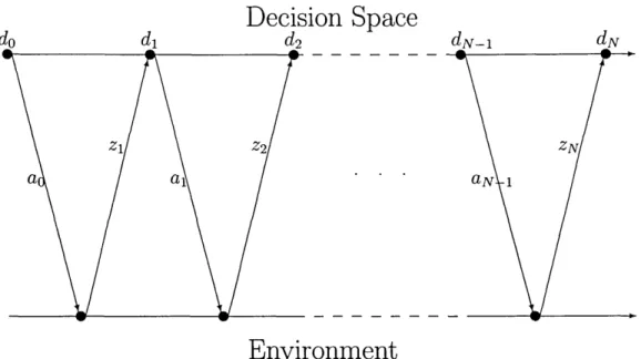
As discussed in section 1.3.3, inference problems for real sensor networks are stochastic optimization problems and can therefore benefit from dynamic analysis. Specifically, breaking the problem into a sequence of actions followed by observations and allowing future actions to depend on previous observations allows for better solutions. A dia-gram of the organization of a dynamic prodia-gram is shown in Figure 2-2. In the figure,

ai

is the

i

th _{action taken,}

_d

i

is the

i

th _{decision and}

_Zi

_{is the}

_i

th

sensor measurement received.

Our dynamic optimization equation is then

J(

7r

t)

= min

(E[t(a)]

+

L

p(z)

*

J(f(7rt,

Z,Pi(Z\X)))])

(2.3)

aEAt

do

Decision Space

d

2

Environment

Figure 2-2: Dynamic decision flow

with

J(7rt)

=

0 if

J-L(7rt) ::;

1, and where 7rt is the posterior density at time

t, t(a)

is

the time it takes to perform action

a, p(z)

= L:xEX

p(x)

*

Pi(zlx)

and

f(7r,

z,p(zlx))

is the state update function defined by the inference problem (see Section 2.1).

2.4

Solution to the Minimum Time Formulation

In most cases, solving dynamic programs like that represented in Equation 2.3 re-quires an insupportable amount of computation, necessitating the adoption of ap-proximate methods, such as heuristics. However, under certain assumptions optimal solutions can be determined a priori. In Section 2.4.1 a sensor network in which all measurements are predetermined is examined. It is shown that if only one sen-sor can be queried or deployed at a time and when

J-L(

7rt) - 1 is large relative to

E_z

[J-L(7rt) - J-L(f(7rt,Z,Pi(zlx)))]'

the optimal action is the one which maximizes the expected rate of decrease of

J-L(

7rt).

Then, in Section 2.4.2, the solution is extended to a limited number of stochastic sensor networks, in which measurements are not predetermined. By analyzing this limited set of (frankly, unrealistic) sensor networks, it is hoped that a heuristic can

be developed for the general problem of time optimal inference in a sensor network.

2.4.1

Optimal Actions in Deterministic Networks

Consider a deterministic sensor network. For each sensor and each mode of operation

(Si, m),

S

E S, m E

_Mi

there is a predetermined measurement

z.

This corresponds to a network where

{

I if

z

E

Zi (

m)

Pi(zlx; m)

=

o

otherwise

Furthermore, let the state update equation f(7rt,

z,pi(zlx;

m) be such that

Thus, for a given sensor and mode of operation the quality measure decreases by a constant amount.

As before let an action a be the 2-pIe

(Si,

m) and consider for the moment only discrete sensor modes. The set of all possible actions for the sensor network is A =

USiES{(Si,

m)}mEMi

and the total number of possible actions is

IAI

=

I::1~1IMil

=

N.

For each action ai

=

(Sj,

m) denote /Li

=

C(Sj,

m) and denote the time necessary for action

ai

as

t

i.

Equation 2.3 can be reformulated as

(2.4)

where

J(7rt)

=

0 if

/L(7rt) ::;

'Y and expectations and the dependance of the state update equation on

Pi(zlx;

m) have been dropped because of the deterministic assumption.

A pure strategy,

Ui,

is one in which action

ai

is used exclusively. The cost asso-ciated with a pure strategy is denoted JUi

(7rt).

Let

J* (7r)

be the optimal cost function

for probability 7r. The maximal information acquisition rate principle states that,

under certain conditions, an optimal action is the one with maximium information acquisition rate (JAR), where the JAR is defined as Pi

=

'i:-Proposition 2.1 For large enough T, if J*(-rr)

>

T,

.* /1i

~ =

argmax-iEN

t

_i

Proof: Assume, WLOG that actions are ordered by

(2.5)

Also, let D

=

(/1(1f) -')').

Consider the (non-existant) instantaneous action

a2

with IAR

ih = 'g

and its associated pure strategy U2. The cost of strategy U2 is

(2.6)

Let J~:N]

(1f)

be the cost associated with the optimal strategy among all strategies

that don't include action al' I will first show that

(2.7)

Then I will show that, for D large enough,

(2.8)

Proof of Equation

2.7

I will prove Equation 2.7 inductively on the number of times and action other than

a2

is taken. For the base case consider strategy al where action ai, iE [2 :

N]

is taken

where the last step was accomplished by substitution from Equation 2.6. Now, by 2.5

(2.10)

Combining Equations 2.9 and 2.10 we get

(2.11 )

For the induction step, consider strategies O'k and O'k+l. Under O'k, k actions other

than 0,2 are taken. By an argument similar to the base case

Then, from Equation 2.10 it's obvious that

Thus

For a1l1r, the optimal strategy among all strategies that don't include al is in O'k for

some k. Therefore Proof of Equation 2.8 Repeating Equation 2.6 D D

J

U2

(1f)

=

-t

2

=

-J.L2 P2

Consider the pure strategy Ul in which only action al is taken. The cost for strategy

By simple algebra we have

(2.13)

If7r is such that

then, from Equations 2.6 and 2.13

(2.14)

Together, Equations 2.7 and 2.8 imply that, if

J-l(7r) - /

is large with respect to the inverse difference of the inverse of the two greatest lARs, then the optimal action sequence will include the action with maximum IAR. Furthermore, since all results of actions are deterministic, action order is superflous. Therefore if

'l

=

arg max Pi iE[l:N]

then action ai is an optimal action for the network.

The maximum network IAR is what is called a dynamic allocation index, or a Git-tens index [15]. GitGit-tens' indices are solutions to a wide range of dynamic problems in which time is a factor. It should be noted that the inference problems in sensor networks do not generally satisfy the requirements for an optimal Gittens index so-lution. Particularly, if the sensor model for the network is not known, but is being discovered, then the index solution dervied above may be significantly suboptimal.

2.4.2

Optimal Actions in Stochastic Networks

We can extend the above analysis to include cases in which both the time required to take each action, ti, and the subsequent decrease in uncertainty for the inference

problem, J-li, are random variables. Making these values random variables allows for a more realistic representation of a sensor network. Results similar to those from

Section 2.4.1 can be derived as long as the random variables are assumed independent. First, the results will be extended to stationary systems where the expected values of the random variables remain constant, then to a set of interesting, non-stationary systems.

Stationary Systems

In the case of stochastic systems with constant mean, the cost function 2.3 can be written as

(2.15) where

J(7r)

=

0 if

J-L(7r) ::; ,.

This is exactly equivalent to Equation 2.4 except that the cost is now taken under an expectation on both the immediate time cost of action i as well as on the future cost-to-go.

Proposition 2.2 For large enough T, if

J*(7r)

>

T,

i* =arg ~ax E[ J-Li] tEN

t

_i

Proal

Since E[J-Li] and E[ti] are assumed independent the cost of pure strategy Ui is

(2.16)

J

Ui

(7r)

can be bounded by

where Pi =

71-.

Again, assuming Equation 2.5 and assuming that

we have the result

where U2 is the instantaneous pure strategy with IAR equal to P2. Consider the space of all strategies that only include actions

a[2:N]

as well as action

a2.

The cost for strategy a from that space is

(2.18)

where

ai

represents the number of times

ai

is taken (to simplify math, al is assumed

to be the number of times action

a2

is taken) and

Di

=

E[/Li]

*

ai.

Since

P2

>

P3

>

... >

PN

(2.19)

Furthermore, since action

a2

has instantaneous cost N V Jr 3 a s.t.

D

=

(/L(Jr)

-,)

=

L:Di

i=l

Equations 2.17 and 2.19 together imply that, for

D

large enough and for constant and independent

E[/Li], E[ti]

Vi, an optimal action is the one that maximizes

E[Pi].

Non-stationary Systems

Sensor systems are, in general, non-stationary. If sensor Si is queried once, the

ex-pected decrease in uncertainty is

/Li. If

sensor

Si

is queried again with the same param-eters the expected uncertainty decrease will not generally be

/Li.

To more acurately model the decreasing utility of actions, the following non-stationarity assumption will be made.

Assumption 2.1

Each time action ai is taken, the corresponding

expectation

of

de-crease in uncertainty,

E[/Li] contracts

by a. All other random

variables

remain

sta-tionary.

but the expected decrease in uncertainty is no longer constant.

Let

U

be a vector such that

Ui

is the number of times

ai

is taken. Also, denote the initial expected decrease in uncertainty due to action

ai

as

E[J.li].

If the initial uncertainty of the system is

J.l( 7r),

the expected uncertainty after taking the actions specified by U is N ai-1

J.l( 7r) -

2:

(E[J.li]

2:

0/)

i=l

j=O N 1 a.

-

J.l(7r) -

2:

(E[J.li]

*

1~ aa l )

i=l

(2.20) (2.21)

The expected time under strategy U can be written as

N J

a(7r)

=

2:

UiE[ti]

i=l

with the understanding that

E[J.lClra)]

::; ,].

The optimal cost can be written

which can, in turn be rewritten as the program

where D

=

J.l( 7r) - ,.

Since

a

is constant, the constraint can be rewritten as N

2:

(E[J.li]

*

(1 - aa

i ))

>

D(l - a)

i=l

N

2:

(E[J.ld

- E[J.li]aa

i ))

>

D(l -

a)

i=l

N

D(l - a) ~

I:

E[/li]

i=l

The constraint is non-linear in 0". Consider instead the linearized system, where the

aO"i terms are linearized about the nominal point

O"?

= O. The resulting constraint is

N

I:

(E[/ld

- E[/li] (Ina )O"i

>

D(l-

a)

(2.22)

i=l

N N

-(lna)

*

I:E[/li](O"i)

>

D(l - a) -

I:

E[/li]

(2.23)

i=l

i=l

N

1 N

I:

E[/li]( O"i) >

-(I:

E[/li] -

D(l-

a))

(2.24)

lna

i=l

i=l

where, in the final step, the inequality doesn't change directions since - In a

>

O.

The constraint is now the same as in the stationary case, except that strategy

0"

must

satisfy Equation 2.24 rather than

2:[:1

E[/li] (O"i)~

D.

Letting

_ 1 N

D

=

In a

(I:

E[/li] -

D(l -

a))

i=l

the analysis for the stationary case demonstrates that an optimal action for the

lin-earized system is the one that maximizes the expected IAR. Unlike the systems

ana-lyzed previously, this may not always be the same action, due to the decreasing value

One caveat must be made in non-stationary systems that follow the model

de-scribed above. Due to the asymptotic properties of the expected decreases in

un-certainty, it is possible that the set of feasible solutions to the dynamic program is

empty. If

2:[:1

E[/li] (l~a) ::;

D

there is no action sequence that leads to a solution of

sufficient expected certainty. This can be addressed by adding the system constraint

that

2.5

Conclusions

We have shown that in specific types of sensor networks when the distance between the current uncertainty and the threshold is large, the optimal action is the one that maximizes the rate of information acquisiton. This can be compared to the results in [41] where IDSQ is extended to include communication costs. While the above discussion focused on costs due to time, it could be easily extended to situations where the main cost is communication as in the networks considered in [22, 41]. In Chapter 4 the IDSQ algorithm will be compared to the above formulation through simulation.

The maximum IAR principle is particularly well-suited to sensor network appli-cations because it can be implemented in a distributed fashion. Because the optimal solution is the one with maximum IAR, if the assumption is made that a sensor's IAR is independent of other sensors, each sensor can calculate its own optimal IAR among all its possible modes of operation. A distributed leader election algorithm [23] can then be used to nominate the sensor with maximum individual JAR. Finding the maximum IAR for a single sensor will generally involve a non-linear optimization problem. Interior point methods [4] and randomized solution methods may need to be used in order to find the operating mode with maximum JAR. Due to the com-plexity of the solution methods, finding the utility of the maximum IAR method may be limited to sensors with significant computational ability.

One assumption made in the much of the sensor network literature (e.g. [9,27,41]) as well as in the preceeding derivation of the maximum IAR principle, is that only one sensor, called the leader, is active in a network at any given time. In networks where the primary goal is to approximately solve an inference problme in minimum time this assumption may be prohibatively limiting. Chapter 3 will show how to extend the principle of maximum IAR to networks in which several sensors can operate simultaneously in order to cooperatively solve the given inference problem.