Optimized and robust experimental design: a non-linear application
to EM sounding
Hansruedi Maurer1 and David E. Boerner2
1 Institute of Geophysics, ET H-Ho¨nggerberg, 8093 Zu¨rich, Switzerland. E-mail: [email protected] 2 Geological Survey of Canada, 1 Observatory Cres., Ottawa, ON, Canada, K1A 0Y3
Accepted 1997 August 14. Received 1997 July 17; in original form 1997 March 10
S U M M A R Y
Pragmatic experimental design requires objective consideration of several classes of information including the survey goals, the range of expected Earth responses, acqui-sition costs, instrumental capabilities, experimental conditions and logistics. In this study we consider the ramifications of maximizing model parameter resolution through non-linear experimental design. Global optimization theory is employed to examine and rank different EM sounding survey designs in terms of model resolution as defined by linearized inverse theory. By studying both theoretically optimal and heuristic experimental survey configurations for various quantities of data, it is shown that design optimization is critical for minimizing model variance estimates, and is particu-larly important when the inverse problem becomes nearly underdetermined. We introduce the concept of robustness so that survey designs are relatively immune to the presence of potential bias errors in important data. Bias may arise during practical measurement, or from designing a survey using an appropriate model.
Key words: electromagnetic sounding, experimental design, inversion, robust statistics.
the published studies illustrate the universality of this concept
1 I N T R O D U C T I O N
within geophysics. For example, Glenn & Ward (1976) and Jones & Foster (1986) employed linearized inverse theory for Geophysical experimental design is fundamentally based on
our ability to understand the physical laws relating Earth designing electromagnetic surveys over layered conductivity structures. Barth & Wunsch (1990) designed marine seismic properties to measurable data. This experience is usually gained
through a combination of theoretical investigations, repeated experiments, and Hardt & Scherbaum (1994) determined opti-mal earthquake network configurations. More recently, Curtis simulations with simple numerical or analogue models and
interpretation of previous field surveys. While extremely power- & Snieder (1997) determined the model parametrization that led to the optimal model resolution. We augment these previous ful, heuristic experimental design can be limited, particularly
by the degree of specialization required to understand the studies by considering that pragmatic designs should also allow constraints due to cost and logistics, while admitting the subtleties of applying geophysical techniques in complicated
environments. Heuristic designs are further complicated by possibility of data error. Our aim here is to design a practical experiment that optimally resolves important features in the variations in socio–environmental, logistical or instrumental
constraints between surveys. The ultimate goal of all geophysi- Earth (within the limits imposed by the physical method). We examine the influence of minimizing data acquisition costs cal surveys is that resolution of Earth structures should be
limited only by the capabilities of the geophysical method, and (that is collecting less data) on the design process by quantifying the corresponding degradation of model resolution. Moreover, not by inappropriate survey layouts or insufficient data.
Philosophically, we desire an ‘optimal’ data set. Understanding we develop a method to design experiments that are robust in the sense that small variations in the design, or the presence that no better data could have been acquired (within the
experimental constraints) is extremely powerful as it dramati- of bias errors in the data, do not unduly compromise the survey objectives.
cally expands the scope and importance of forward
model-ling by providing additional rigour to feasibility studies, Experimental design is based on an expected inverse problem (that is some knowledge of the Earth is assumed, but there is instrumentation design and survey costing.
In this paper, we consider the issues surrounding the quanti- no data to interpret). Conducting geophysical surveys admits that the a priori information is incomplete, thus raising import-tative design of an ‘optimal’ survey. Our particular goal is to
maximize the formal resolution of model parameters. Designing ant concerns about inappropriate models or assumptions affecting the design. For this reason, experimental design is experiments that enhance model resolution is not new, and
perhaps best viewed as an iterative exercise in hypothesis
2 T H E O R Y
testing (Fig. 1). The design process involves the delineation of
data space regions that are either critical or unimportant for In establishing the experimental design procedure, we assume that the model parameter resolution is expressed in terms of resolving the model parameters, presumably for a range of
models. The decisive advantage of planning surveys with linearized inverse theory. In contrast, the non-linear optimiz-ation process of actually selecting the experimental layout is experimental design techniques is that information and
assumptions can be examined, tested and considered before performed using a genetic algorithm. As both techniques are well described in the literature, the cursory introduction that incurring data acquisition expenses. However, non-linear
relationships between the observed data and the causative follows serves only to introduce notation and key concepts as applied to experimental design. Additional details about the model can limit the applicability of experimental design. For
this reason we consider the issue of non-linearity in our individual methods can be found in several excellent texts (e.g. Menke 1984; Tarantola 1987; Sen & Stoffa 1995).
example design study.
Following, Barth & Wunsch (1990), Hardt & Scherbaum (1994) and Curtis & Snieder (1997), we design the experiment
2.1 Linearized inverse theory
objectives by formulating a constrained global optimization
problem (Fig. 1). The formal resolution of model parameters is Non-linear physical experiments are generally governed by a determined through linearized inversion and forms the basis functional g(m):
of quantifying acceptable survey designs. Thus any geophysical
dobs=g(m)+e (1)
technique that is Fre´chet differentiable can be subjected to this
experimental design procedure. Our test case is a frequency relating observed data dobs, model parameters m, and errors domain electromagnetic (EM) survey of layered Earth struc- e. The well-known solution of the linearized inverse problem tures. EM methods are strongly non-linear and admirably corresponding to eq. (1) (e.g. Menke 1984) can be written as suited to investigate the robustness of design studies to
inappro-m=m
o+G−1Dd , (2)
priate expectations of the Earth. Diffusive EM methods pose problems for model resolution and yet, for layered earth
where mo is an initial model, G−1 a generalized inverse matrix models, are simple enough to understand the results of the and Dd the difference between observed and predicted data. optimization in detail. In addition to studying model reso- The generalized inverse G−1 can be, for example, determined lution, we address the important issue of designing robust
using singular value decomposition (Lanczos 1961; Lawson & experiments. Pragmatic survey design must constrain
subsur-Hanson 1974): face models while not being susceptible to gross data errors
or model inadequacies at potentially important data points. G−1=VL−1UT , (3)
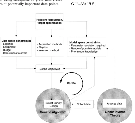
Figure 1. Schematic overview of general experimental design, showing components involved and their relationships. Notice that the genetic algorithm (GA) is used only to select the optimal experimental design, while standard linearized inverse theory is used to characterize the formal model resolution. In this paper we consider only model resolution, costs and robustness in defining the design objective.
where the matrix U contains a set of orthonormal vectors that Darwinian selection should evolve the whole population to a higher degree of fitness. The definition of a single objective span the data space, and the columns of matrix V are
orthonor-mal vectors that span the model space (Menke 1984). The function means that genetic algorithms tend to reduce diversity within the population, and so the output of the GA runs was diagonal matrix L contains the singular values describing the
relationship between the data space and the model space. carefully examined to ensure convergence had been reached. Singular value decomposition also results in a simple form of
the model covariance matrix:
2.3 Experimental design
CM=CDVL−2VT , (4)
Physical laws, past experience with data inversion, and/or which describes the model-space mapping of the data variances simulations with synthetic data govern experimental design.
CD into a posteriori model parameter uncertainties (e.g. However, quantifying this procedure in a numerical procedure Menke 1984). by iterating on a single design component is inefficient and The matrix H describes the data-space mapping between the may not lead to an optimal design (Fisher 1925). As an observed data dobs and the predicted data dpre (e.g. Hoaglin & alternative, we follow the suggestion of Fisher (1925) and Welsch 1978; Menke 1984): impose some randomness on the design specifications through the genetic algorithm formulation. Evolution starting from a
dpre=Hdobs , where H=UUT . (5)
broad range of diverse designs should lead to the culling of the unfit and selection of those designs that have optimal In the geophysical literature, H is also known as the data
components (that is leading to the smallest objective function). resolution matrix (Menke 1984) or the information density matrix
Statistical experimental design identifies data acquisition (Wiggins 1972). H is a projection matrix and is symmetric and
parameters (for example source–receiver configurations, band-idempotent i.e. H=H2 (Staudte & Sheather 1990). It follows
width, acceptable signal to noise ratios) that ‘optimally’ deter-from these properties that the length squared of the ith column
mine a particular subsurface model. Our approach is shown vector Hi is equal to hii. Furthermore, the trace of H is schematically in Fig. 1. The first step is to construct a hypotheti-cal a priori subsurface model (or range of models, if sufficient tr(H)= ∑N
i=1 h
ii=M , (6) uncertainty regarding the Earth exists). The desired model resolution then becomes a constraint that defines the space where N is the number of data points and M is the number
(genetic algorithm population) available to search for the best of unknown model parameters. Since the diagonal elements of
data acquisition configuration.
H describe the relative importance (that is the ability of
The objective function, C, defines ‘optimal’ in a mathematical influencing model parameters by small perturbations of the
sense. In our case, C shows how the data from a particular data value) of a particular data point, diag(H) is called data
survey layout resolve the parameters of a hypothetical a priori importance (Menke 1984). From eq. (6) it follows that the
subsurface model. An appropriate objective function definition average importance of a data point is M/N. When an element
is the critical element of experimental design. We must charac-of diag(H) is significantly larger than the remaining h
iivalues, terize, with a single number, the quality of a particular design the associated datum is called a leverage point. Data errors at
configuration. As the data will be analysed with linearized a leverage point can strongly affect the inversion result (e.g.
inversion theory, one reasonable objective function could Staudte & Sheather 1990). In robust regression analysis,
minimize the a posteriori covariances CM for all subsurface leverage points are avoided whenever possible by adopting a
model parameters (eq. 4). Since CM is a function of L−2, we process called equileverage design (Staudte & Sheather 1990).
have defined an objective function C as
2.2 Genetic algorithms C= ∑M i=1 1 L2 i +d , (7)
For strongly non-linear optimization problems, or for
situ-where d is a positive constant. This definition has several ations in which the partial derivatives of g(m) cannot be easily
desirable properties. formed, global optimizers provide a useful alternative to linear
inverse methods (e.g. Sen & Stoffa 1995). An important class
(1) C is directly and simply related to CM. of global optimizers, genetic algorithms (GA), were originally
(2) Since C is most sensitive to small singular values, the proposed by Holland (1975). To some extent a genetic
algor-algorithm represents an attempt to reduce the underdetermined ithm simulates biological evolution. The goal is to ensure the
components in the inverse problem (eq. 7). progeny of the most fit members survive through successive
(3) In case of an inherent ambiguity in the inverse problem generations. The algorithm is formulated as follows:
(zero or nearly zero singular values), C ensures that any resolvable subsurface model parameters are well constrained (1) initiate a random population, each of which represents
a particular geophysical survey design (encoded as a bit string); ( but perhaps not optimally resolved).
(4) The parameterd in eq. (7) can be selected to match the (2) evaluate the ‘fitness’ (misfit between predicted and
observed data|dobs−g(m)|k, where k is an arbitrary constant) expected noise characteristics of the observed data. In the case of error-free data,d should be so small that it only prevents C of the population members via an objective function defined
in terms of model resolution and any additional constraints; from going to infinity and keeps the algorithm numerically stable. If the expected noise level is significant, d should be (3) procreate a new generation after selecting the most fit
parents and applying genetic operators (crossover, mutation chosen large enough such that the objective function C ignores singular values associated with unresolvable components of and replication);
There are many other objective functions that minimize model covariances. Appendix A provides a comparison of our choice in eq. (7) with some other definitions found in the literature. For minimizing the objective function C (eq. 7) we have used a library of genetic algorithms developed by Hunter (1995). Appendix B provides more information on parameter settings, convergence speed and other properties of the individual GA runs.
3 E X P E R I M E N TA L D E S I G N O F A F R E Q U E N C Y- D O M A I N E M SU R V E Y
3.1 The experiment
Simulating a simple controlled-source EM survey is useful for exploring the characteristics of experimental design. A hori-zontal electric dipole (HED) source is placed at the surface of a layered half-space. The data comprise vertical magnetic field measurements at various positions between 0.1 and 1000 m from the source (Fig. 2). The frequency range lies between 1 Hz and 1 MHz, although the quasi-static limit has been imposed, thus preventing radiative propagation of the
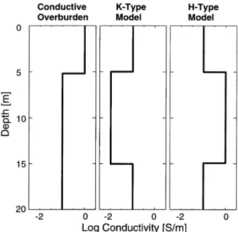
high-Figure 3. Conductivity models used in this study.
frequency EM fields. This source–receiver configuration has a cylindrical symmetry modulated by sinh (Fig. 2), so we consider that the experimental design parameters are simply frequency
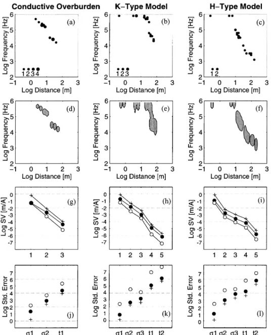
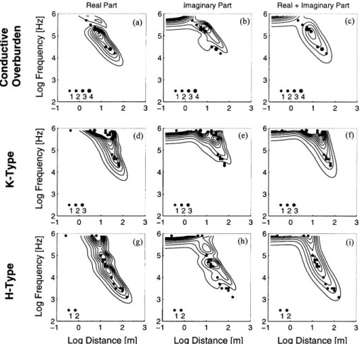
( f ) and distance (r). Three simple 1-D earth models (Fig. 3) Figs 4(a)–(c) show the best receiver configurations in ( f,r) space selected by the genetic algorithm for each of the test are used to illustrate the experimental design procedure.
Sampling is logarithmic with 10 samples per decade, giving a models. In other words, these locations are optimal for resolv-ing the model parameters accordresolv-ing to the objective function total of 2400 possible receiver configurations (60 frequencies
and 40 distances). Actually acquiring such a large number of (7) and for 20 data. Desirable measurement locations for all models tend to cluster along relatively narrow diagonal bands frequency–distance estimates would be impractical, but is
necessary to provide a reasonably large model space for the in frequency–distance space, roughly along lines of constant induction number (e.g. Ward & Hohmann, 1988). For the optimization algorithm to explore. Fre´chet differentiability
for this non-linear class of models and EM methods was conductive overburden and the K-type model, the information is mostly concentrated at higher frequencies (above 10 kHz), established by Chave (1984).
reflecting the presence of a relatively conductive surface layer, whereas the H-type model also includes lower-frequency
3.2 Minimization of a posteriori error estimates
regions.
Although the earth models are quite different, the data The data in this experiment are assumed to be error-free, of
unlimited bandwidth and accurate to computer precision. sampling configurations in Figs 4(a)–(c) exhibit relatively con-sistent and confined patterns, delineating well-defined regions Thus, thed parameter in eq. (7) is kept small (10−20). We seek
to find the optimal data subset consisting of 20 points in ( f,r) that contain most of the information about the subsurface. This observation is reinforced by examining the fittest individ-space. When distributed adequately, this subset size should
result in a moderately overdetermined system of equations, uals of the final generation. Figs 4(d)–(f ) show areas that include 99.9 per cent of ( f,r) pairs belonging to the fittest 10 sufficient to constrain each of the test models (which have at
most five free parameters). per cent of the final population. Although genetic algorithms tend to homogenize populations (Hunter 1995), there is some diversity shown in Figs 4(d)–(f ), yet the delimited areas cluster within and around those already identified by the fittest structures (Figs 4a–c).
A physical interpretation of the regions delineated by the genetic algorithm is straightforward. The selected ( f,r) points fall in the transition between the electromagnetic near field and far field, or at the electromagnetic inductive limit, the data regions most sensitive to changes in the conductive parts of the models (Boerner & West 1989). Note that the genetic algorithm solution considers the resolution of all model param-eters simultaneously, and thus is a more refined sampling of ( f,r) space than the single-parameter example shown by Boerner & West (1989). As the transition zone is narrow, the genetic algorithm tends to duplicate important data points,
Figure 2. Schematic representation of the simulated EM experiment.
Figure 4. Experimental design through minimization of a posteriori model variances. Plots (a) to (c) show the optimal distribution of ( f,r) pairs for the different conductivity models. Duplicated data points are represented with larger dots (see legend). (d)–(f ) Regions of desirable locations for the fittest 10 per cent of the final GA population. The shaded areas delimit regions containing 99.9 per cent of all ( f,r) pairs. (g)–(i) Singular-value spectra for the complete data set (+), the random solution (#) and the GA solution ($). ( j)–(l) A posteriori error estimates for the complete data set (+), the random solution (#) and the GA solution ($). s1 to s3 denote layer conductivities and t1 and t2 layer thicknesses.
(Fig. 4a). While perfectly legitimate in synthetic studies, dupli- approach those of the random solution for all models, as expected from the definition of the objective function (eq. 7). cation is not desirable for real survey designs, as discussed
below. While singular-value spectra form an interesting basis for appraising the properties of the genetic algorithm, the corre-To study quantitatively the properties and reliability of the
genetic algorithm, we compare the singular-value spectrums sponding standard errors of model parameters allow a formal comparison based on the objective function. Figs 4( j)–(l ) and a posteriori covariance estimates based on the best genetic
algorithm solution with those of other survey designs. The depict the standard errors of the model parameters (defined as the square root of the diagonal elements of the model covari-complete data set of all 2400 ( f,r) pairs approximates the best
attainable experiment, while a randomly selected subset of 20 ance matrix, assuming the data variance CD=s2I in eq. 4). The individual panels of Figs 4( j)–( l ) reveal that by judicious data points should approach the worst case (completely naive
sampling) limit. Figs 4(g)–(i) show that the shapes of the selection of<1 per cent of the complete data set, the corre-sponding standard errors differ on average by less than a singular value spectra are generally similar for the three cases,
but there are large differences in the magnitudes. Note that factor of five. Genetic algorithm solutions are better, on average, by a factor of 30 compared with the random solutions. the largest singular values for the genetic algorithm solution
As already noted for the singular-value spectra, we also observe value spectrum. Conversely, the objective function preferen-tially selects configurations that improve the resolution of considerable deviations from these average values.
poorly resolved model parameters. When the well-resolvable parameters are the primary survey target, the objective function
3.3 Influence of the subset size
should be modified accordingly. Since the amount of data acquired is usually related to the
survey costs, it is often desirable to minimize the data volume.
3.4 Analysis of data importance
Experimental design offers an opportunity to examine the
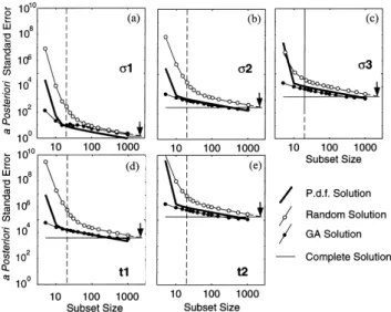
trade-off between data quantity and model parameter reso- The objective function developed above is based solely on lution. As a test case, we consider the H-type model using the resolving the details of the model space. An alternative, but complete and genetic algorithm data sets together with a important, context is to consider objective functions in the random data set. data space. In particular, we examine the role of data impor-Figs 5(a)–(e) show the a posteriori standard error estimates tance, expressed as the diag(H) (eqs 5 and 6). Comparisons of for the individual model parameters as functions of subset size. the genetic algorithm solutions (Figs 4a–c) with the importance For larger subset sizes, the standard errors of the random and values for the complete data set in frequency–distance space the genetic algorithm solutions exhibit a power-law decay are shown in Fig. 6. While the real and imaginary parts of the proportional to the square root of the subset size, as expected vertical magnetic field are treated equally in the genetic algor-for a purely overdetermined inverse problem. Note that dupli- ithm objective function, it is interesting to identify the contri-cation of important data points in larger subsets allows the butions of the individual components to the experimental error estimated from the genetic algorithm solution to be design. Most of the information from the real part of H
z is smaller than that of the complete data set (Fig. 5e). contained in a relatively narrow distance range (Figs 6a, d and Deviations from the power-law behaviour occur for the g), whereas the imaginary parts provide additional information random solutions at smaller subset sizes, indicating the occur- in the high-frequency range at shorter distances (Figs 6b, e rence of significant underdetermined components in the inverse and h).
problem. Interestingly, the standard errors of the genetic Figs 6(c), (f ) and (i) display the genetic algorithm solutions algorithm solutions are inversely proportional to the square superimposed on the data importance contours, averaged for root of N (subset size) over the entire subset size range. This the real and imaginary parts. The strong correlation between observation indicates that design optimization has succeeded large importance values and the GA solution suggests that the in keeping the inverse problem for the conductivity structure importance distribution could be used as a probability density overdetermined, almost independently of subset size. A pos- function (pdf ) for selecting an optimal ‘random’ data set. Since teriori errors for the first layer conductivity do deviate from a the calculation of diag(H) involves only the calculation of N power-law decay for smaller subsets, approaching the error scalar vector products with length M, experimental design level of the random solution (Fig. 5a). Because the first-layer based on data importance would be computationally much conductivity is the best-resolved parameter (cf. y-axis in Fig. 5), less demanding than the GA solution (requiring multiple it is primarily determined by the largest values in the singular- singular-value decompositions). Using an importance pdf is much like defining a new objective function, focused primarily on resolving parameters associated with large singular values. In fact, exploiting the important data space in this fashion is quite close to the process of heuristic experimental design. An experienced geophysicist would have discovered that the trans-ition zone of the EM fields is the most important region of the data space, and could design an experiment to sample this space.
Selecting a ‘random’ design using the H matrix as a pdf for determining measurement points was tested for the subset size experiment (also shown in Fig. 5). Generally, the results are comparable with those of the GA solution, but with two significant differences.
(1) When the subset sizes approach the underdetermined case (<5 frequency–receiver pairs=10 constraining equations), the pdf solution degrades markedly. Lacking information about interrelationships between data points limits the usefulness of the pdf experimental design to purely overdetermined problems.
Figure 5. Influence of the data acquisition subset size (i.e. cost). (2) The first-layer conductivity is better resolved for larger Linear extrapolation of the curve for random survey designs intersects
subsets with the importance pdf than by the genetic algorithm
that of the complete data set at a subset size of 2400 (=size of the
solution. Since data importance is governed mainly by
well-complete data set) and is marked with an arrow. The vertical dashed
resolvable parameters, the pdf approach is most effective for
line indicates a subset size of 20.s1, s2 and s3 denote layer
conductivit-constraining these parameters, whereas the objective function
ies and t1 and t2 layer thicknesses. The heavy lines represent the
in the genetic algorithm tries to resolve all parameters.
solution derived by selecting a design using H as a probability
Figure 6. Contour plots of the data importance superimposed on the best configuration determined with the GA (Figs 4a–c). The contour lines are linearly spaced between 0.02 and 0.2. See text for further explanations.
parameters are slightly higher than those of the GA solution tance spread lie between 0 and 1, whereas C can vary over several orders of magnitudes. Accordingly, we restrict the (Figs 5c and e).
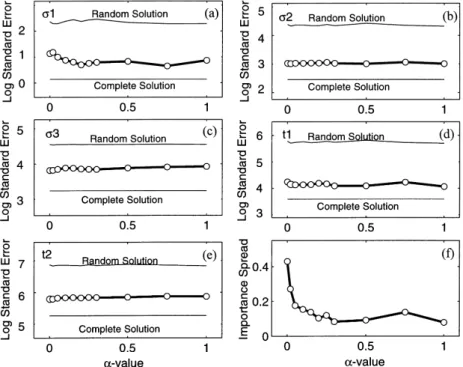
numerical range of C through the use of log(C ) (eq. 8). The limitations observed for the pdf solution probably reflect The efficiency of equileverage design for the case of the the results of heuristic experimental design. H-type model is shown in Fig. 7(f ). There is a decrease of importance spread as a increases. Even for small values of a the occurrence of leverage points is effectively suppressed. Figs
3.5 Equileverage design 7(a)–(e) show standard errors as a function ofa and
demon-strate that equileverage configurations constrain potentially Experimental design, as outlined so far, is basically a process
well-resolvable parameters even better than non-robust designs of locating data points important to the model resolution, or,
(Fig. 4). This apparent paradox can be explained by consider-in terms of robust statistics, selectconsider-ing leverage poconsider-ints (e.g.
ing eq. (6), which explains why penalizing a large importance Staudte & Sheather 1990). However, severe repercussions in
spread (Hmaxii −Hminii ) not only avoids leverage points, but also terms of parameter estimation could result from even minor
prevents the incorporation of unimportant data. Consequently, data errors at a leverage point. Alternatively, an inappropriate
minimizing the importance spread in the data space can be a expected model could introduce an effective bias into the
powerful tool for improving the experimental design. design, and this bias would be most evident at leverage points.
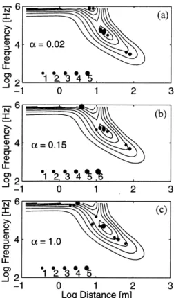
Figs 8(a)–(c) display optimal ( f,r) points superimposed on Consequently, it is desirable to find survey designs that
mini-the importance distribution for different values of a, showing mize a posteriori variances, but that do not rely exclusively on
that the equileverage design algorithm tends to duplicate data leverage points.
(that is such that all data have equal importance). In the Equileverage constraints require a redefinition of the
objec-presence of unbiased random data errors, repeat recordings of tive function to penalize leverage points (Staudte & Sheather
the same data point improve data precision. However, this 1990). We define a modified objective function:
concept is already applied in standard instrumentation and recording practices. It may be better, from the design point of C*=log(C)+a(Hmax
ii −Hminii ) , (8) view, to assume that data are recorded to the best obtainable where (Hmaxii −Hminii ) denotes the importance spread anda is precision and that repeat measurements do not reduce random error. Whereas data duplication in design studies indicates an arbitrary positive constant. Possible values of the
impor-Figure 7. (a)–(e) A posteriori error estimates of an equileverage design for the H-type model. Error estimates are plotted as a function of thea value defined in eq. (8). Error levels of the complete data set and the random solution are shown as a reference. Note the different ordinate scales of the individual panels. (f ) Importance spread plotted as a function ofa (see eq. 8). s1 to s3 denote layer conductivities and t1 and t2 layer thicknesses.
3.6 Restricting duplication
Data duplication can be suppressed in experimental design. We have chosen to multiply the objective function by a positive constantb>1,
C**=[log(C)+a(Hmax
ii −Hminii )]bp , (9) raised to the power p, where p is the total number of data point duplications. For the H-type model, an empirically determined value ofb=1.1 has proved suitable for eliminating all duplicate points. Fig. 9 shows the equileverage design obtained by employing eq. (9) instead of (8), and Fig. 10 depicts the corresponding error estimates. Data duplication has been curtailed, and the resulting configurations continue to correlate well with the importance distribution. As shown in Figs 9( b) and (c), increasing a tends to spread out the clustering observed around the importance maxima.
There are no significant differences in a posteriori error estimates for the configurations shown in Figs 7 and 10, demonstrating the experimental design optimization problem may be highly ambiguous. In contrast to conventional inver-sion problems, non-uniqueness in experimental design is desir-able because it offers the possibility of imposing additional constraints without degrading the estimated model variances.
4 D I S C U S S I O N A N D C O N C L U S I ON S
Figure 8. Best equileverage design solutions for some selecteda values Inversion to recover a causative model from measured data is superimposed on the data importance of the complete data set.
often mathematically ill-posed (Backus & Gilbert 1968; Jackson 1979) and thus inherently non-unique. The problem is exacerbated by band-limited and inaccurate data. Solution which data require high precision and accuracy, it is also
critical to recognize that we have limited ability in the field non-uniqueness in inverse problems is usually addressed by regularization (e.g. Tikhonov 1963), such that some knowledge to improve arbitrarily the precision of an individual data
tions about the subsurface structure. While additional data in the inverse problem can improve model resolution substan-tially, assumptions do not formally contract the model space allowed by the data. In fact, portions of an inverted model may reflect only the subjective regularization constraints. Experimental design is one means of ensuring that the most appropriate data are acquired, mitigating the requirement for regularization assumptions.
Optimal experimental design complements and extends our heuristic design capabilities by treating operational constraints objectively and reducing personal biases. The benefit of exper-imental design is clearly demonstrated by associating heuristic and data importance pdf experimental design. Experienced experimentalists implicitly understand the role of data impor-tance, yet experiments designed using this approach can unnecessarily degrade model resolution for slightly overdeterm-ined problems, or for weak eigenparameters. Ensuring an overdetermined inverse problem requires not only knowledge of potentially important areas in the data space, but also of the relative interactions of the individual data points. We expect that experimental design will become an important issue in surveys of multidimensional Earth structures, where data acquisition costs serve to make the corresponding inverse problems underdetermined, or only slightly overdetermined.
Heuristic designs cannot include a data robustness criterion. In fact, past experience probably biases the investigator to select leverage points (that is selecting important data regions).
Figure 9. Best solutions of the modified equileverage design (eq. 9) When the important regions of the data space can be
for some selecteda values superimposed on the data importance of adequately sampled, heuristic designs will work quite well. the complete data set. Compare with Figs 6 and 8. However, bias in leverage points can potentially disrupt any
ability to resolve the subsurface, particularly when the data are sufficiently limited that the inverse problem becomes Examples of regularization include step-length minimization
underdetermined. For small data sets, the relative contribution (Marquardt 1970), ad hoc model smoothness (Constable,
of each data point is critical in resolving the model, and the Parker & Constable 1987), and enforcing stochastic
proper-importance pdf-guided ( heuristic) design is inappropriate. It is ties on the medium (e.g. Pilkington & Todoeschuck 1991).
Regularization can be based either on information or assump- important to point out that robustness applies to data errors
Marquardt, D.W., 1970. Generalized inverse, ridge regression, biased
as well as inadequacies of the expected model the design was
linear estimation and nonlinear estimation, T echnometrics, 12,
based on.
591–612.
Experimental design is based on expectations on the
subsur-Menke, W., 1984. Geophysical Data Analysis: Discrete Inverse T heory,
face structure, that is it requires a clear intent and a certain
Academic Press, Orlando, FL.
amount of a priori information. Quantitative designs are thus Pilkington, M. & Todoeschuck, J.P., 1991. Naturally smooth inversions best suited to feasibility studies or follow-up surveys where with a priori information from well logs, Geophysics, 56, 1811–1818. increasing the benefit/cost ratio is highly important. It is Rabinowitz, N. & Steinberg, D.M., 1990. Optimal configuration of a
certainly expedient to consider experimental design when seismographic network: a statistical approach, Bull. seism. Soc. Am., 80, 187–196.
planing additional measurements, or perhaps contemplating
Sen, M.K. & Stoffa, P.L., 1995. Global Optimization Methods in
the use of another geophysical method. On the other
Geophysical Inversion, Elsevier Science, Amsterdam.
hand, experimental design is probably an effective method of
Staudte, R.G. & Sheather, S.J., 1990. Robust Estimation and T esting,
transferring knowledge about the applicability of particular
John Wiley, New York, NY.
geophysical methods to non-specialists. Tarantola, A., 1987. Inverse Problem T heory, Elsevier, Amsterdam.
Tikhonov, A.N., 1963. Regularization of ill-posed problems, Dokl. Akad. Nauk SSR, 153, 1–6.
A C K N O W L E D G M E N T S Ward, S.H. & Hohmann, G.W., 1988. Electromagnetic theory for
geophysical applications, in Electromagnetic Methods in Applied
We thank Alan Green, Klaus Holliger, Alan Jones and Mark
Geophysics, Vol. 1, pp. 131–311, ed. Nabighian, M.N., Soc. Expl.
Pilkington for constructive reviews of the manuscript.
Geophys., Tulsa, OK.
Comments by the two anonymous journal reviewers and editor Wiggins, R.A., 1972. The general linear inverse problem: implication G. Mu¨ller were valuable in clarifying the presentation. We also of surface waves and free oscillations for earth structure, Rev. thank Andrew Hunter for generously making his genetic Geophys., 10, 251–285.
algorithm code available to us. Geological Survey of Canada
publication number 1997058 and Institute of Geophysics, ETH A P PE N D I X A : A LT E R N AT I V E
Zu¨rich, contribution number 979. F O R M U L AT I O N S O F T H E O B J E C T I V E
F U N C T I O N
R E F E R E N C E S There are many different objective functions that can be used
instead of eqs (7), (8) or (9). A simple alternative to our choice
Backus, G. & Gilbert, F., 1968. The resolving power of gross earth
in eq. (7) is to maximize the condition number, defined as
data, Geophys. J. R. astr. Soc., 16, 169–205.
Lminii /Lmaxii . Unfortunately, the condition number can be
maxim-Barth N. H. & Wunsch, C., 1990. Oceanographic experiment design
ized by decreasing the largest SV (singular value) as well as by
by simulated annealing, J. phys. Ocean., 20, 1249–1263.
increasing the smallest SV. A better solution would therefore
Boerner, D.E. & West, G.F., 1989. Spatial and spectral sensitivity
be to consider only Lminii . However, this is not appropriate for
analysis, Geophys. J. Int., 98, 11–21.
Chave, A.D., 1984. The Fre´chet derivatives of electromagnetic induc- problems with undetermined components, i.e. if Lmin
ii =0.
tion, J. geophys. Res., 89, 3373–3380 Other objective functions found in the literature operate on
Constable, S.C., Parker, R.L. & Constable, C.G., 1987. Occam’s the inverse of the Hessian matrix (GTG)−1. Kijko (1977) and inversion: a practical algorithm for generating smooth models from Rabinowitz & Steinberg (1990) proposed the ‘D-criterion’, in electromagnetic sounding data, Geophysics, 52, 279–288. which the volume of the a posteriori model error ellipsoid, Curtis, A. & Snieder, R., 1997. Reconditioning inverse problems using described by 1/√det(GTG), is minimized. Hardt & Scherbaum
the genetic algorithm and revised parameterization, Geophysics, 62,
(1994) implemented an experimental design equivalent to the
1524–1532.
D-criterion by minimizing the product of the eigenvalues of
Fisher, R.A., 1925. Statistical Methods for Research Workers, Oliver &
(GTG)−1. As a variant it is also possible to consider a functional
Boyd, Edinburgh.
that is proportional to the sum of the eigenvalues of (GTG)−1.
Glenn, W.E. & Ward, S.H., 1976. Statistical evaluation of electrical
Curtis & Snieder (1997) have shown that such an approach is
sounding methods. Part I: experimental design, Geophysics, 41,
computationally efficient by virtue of avoiding SVD
1207–1221.
computations.
Hardt, M. & Scherbaum, F., 1994. The design of optimum networks
All these objective functions seek to enhance the magnitude
for aftershock recordings, Geophys. J. Int., 117, 716–726.
Hoaglin, D.C. & Welsch, R., 1978. The hat matrix in regression and of the eigenvalue related to the most poorly resolved model
ANOVA, Am. Stat., 32, 17–22. parameter. In contrast, eq. (7) is most sensitive to the
least-Holland, J.H., 1975. Adaptation in Natural and Artificial Systems, MIT determined eigenparameter of the inverse problem, and this
Press, Boston, MA. could be a function of several model parameters. If the
Hunter, A., 1995. SUGAL User Manual, www5http://osiris. elimination of underdetermined components is the goal of sunderland.ac.uk./ahu/sugal/home.hrml. experimental design, eq. (7) would be the preferred choice. On Jackson, D., 1979. The use of a priori data to resolve non-uniqueness
the other hand, choosing an objective function based on the
in linear inversion, Geophys. J. R. astr. Soc., 57, 137–157.
Hessian matrix is advantageous in experimental designs where
Jones, A.G. & Foster, J.H., 1986. An objective real-time data-adaptive
a particular model parameter has to be resolved with high
technique for efficient model resolution improvement in
magnetotel-accuracy. This can be achieved by introducing a weighting
luric studies, Geophysics, 51, 90–97.
function for the eigenvalues.
Kijko, A., 1977. An algorithm for the optimum distribution of a regional seismic network-1, Pageoph, 115, 999–1009.
Lanczos, C., 1961. L inear DiVerential Operators, Van Nostrand, A P PE N D I X B : T H E G E N E T I C A L G O R I T H M London.
In this study we employed SUGAL, the SUnderland Genetic
Lawson, C.L., Hanson, R.J., 1974. Solving L east-Squares Problems,
Table B1. Relevant input parameters for the SUGAL package. See SUGAL settings and options that are common to all our
User Manual for further information. studies. More information on the individual parameters
can be found in the SUGAL User Manual located at
Parameter Name Parameter Setting www5http://osiris.sunderland.ac.uk./ahu/sugal/home.html.
annealing_temperature 10
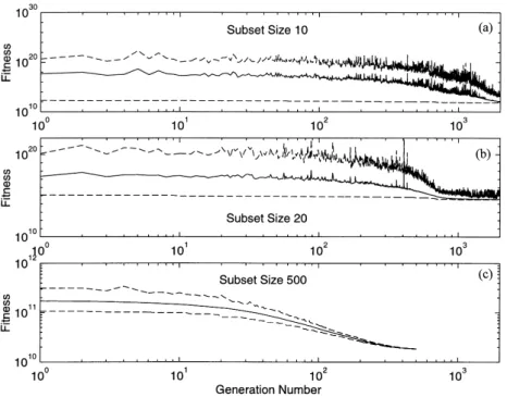
Convergence behaviour is an important aspect of global
annealing_decay 0.95
optimization. In order to determine whether the procedure has
crossover onepoint
converged or not, we analysed the fitness of each generation.
crossover_points 3
Statistical parameters included the fitness of the best and the
elitism on
worst population member as well as an average fitness of the
generations 2000
init uniform whole population. When all of these quantities are similar,
mutation uniform convergence has been achieved. Fig. B1 shows fitness minimum,
population 5000 maximum and average as a function of the generation number
replacement uniform for the subset size experiment depicted in Fig. 5. The individual selection roulette panels reveal that convergence speed is a function of the subset
stop generations
size—the larger the subset, the faster the convergence. This probably reflects the degree of freedom of the different exper-imental designs. Having only a few data points available, there provides wide and easy-to-use support for most of the genetic
algorithm parametrizations found in the literature. SUGAL are only a few configurations that are ‘optimal’ according to the definition of the objective function. With increasing subset also provides an annealing scheme that may improve the
convergence speed. Table B1 summarizes the most important size the variability of desirable configurations increases.
Figure B1. Convergence behaviour of the GA for different subsets (Fig. 5). Fitness of the best and the worst configurations for each generation is plotted with dashed lines, and the average fitness is represented with a solid line.