HAL Id: hal-01612293
https://hal.inria.fr/hal-01612293
Submitted on 6 Oct 2017
HAL is a multi-disciplinary open access
archive for the deposit and dissemination of
sci-entific research documents, whether they are
pub-lished or not. The documents may come from
teaching and research institutions in France or
abroad, or from public or private research centers.
L’archive ouverte pluridisciplinaire HAL, est
destinée au dépôt et à la diffusion de documents
scientifiques de niveau recherche, publiés ou non,
émanant des établissements d’enseignement et de
recherche français ou étrangers, des laboratoires
publics ou privés.
A Formal Proof in Coq of LaSalle’s Invariance Principle
Cyril Cohen, Damien Rouhling
To cite this version:
Cyril Cohen, Damien Rouhling. A Formal Proof in Coq of LaSalle’s Invariance Principle. Interactive
Theorem Proving, Sep 2017, Brasilia, Brazil. �10.1007/978-3-319-66107-0_10�. �hal-01612293�
A Formal Proof in Coq of LaSalle’s Invariance
Principle
Cyril Cohen1 and Damien Rouhling1 Université Côte d’Azur, Inria, France. [email protected], [email protected]
Abstract. Stability analysis of dynamical systems plays an important role in the study of control techniques. LaSalle’s invariance principle is a result about the asymptotic stability of the solutions to a nonlinear system of differential equations and several extensions of this principle have been designed to fit different particular kinds of system. In this paper we present a formalization, in the Coq proof assistant, of a slightly improved version of the original principle. This is a step towards a formal verification of dynamical systems.
Keywords: Formal proofs. Coq. Dynamical systems. Stability
1
Introduction
Computer softwares are increasingly used to control moving objects: robots, planes, self-driving cars. . . This raises security issues, especially for human beings that are in the surroundings of such objects, or even inside them. Control theory brings answers by providing techniques to control the behaviour of dynamical systems. Control theoreticians focus on the mathematical foundation of their techniques. But another important aspect is to check that the implementations of such techniques respect their theoretical semantics.
The Coq proof assistant [23] provides a framework for both implementing functional programs and checking their correctness. It has also proven to be a convenient tool for the formalization of mathematics, for instance through the formalizations of the Four-Color Theorem [9] and of the Odd Order Theorem [10] based on the Mathematical Components library1
and the SSReflect ex-tension of Coq’s tactic language [11].
In this paper we present a formalization in Coq2 of a mathematical result about the asymptotic stability of dynamical systems defined by a nonlinear sys-tem of differential equations: LaSalle’s invariance principle [15]. Stability is an important notion for the control of nonlinear systems [14] and LaSalle’s invari-ance principle or extensions of it have been successfully used to prove stability of different kinds of system [1,8,18,19].
1
https://math-comp.github.io/math-comp/
2
For this formalization, we used the SSReflect tactic language and the Co-quelicot library [3], which extends Coq’s standard library for real analysis [20]. We first present our improvements on the statement of LaSalle’s invariance prin-ciple (Sect. 2), obtained by relaxing constraints on the original statement by LaSalle. Then we discuss details of the formalization (Sect.3). Finally, we give the formal statement of the result we proved (Sect.4) before pointing out the parts of the proof where classical reasoning was necessary (Sect.5).
2
A Stronger Result
The original statement of LaSalle’s invariance principle [15] contains hypothe-ses that can be relaxed and draws a conclusion which is weaker than what has been really proved. In this section, we first state LaSalle’s invariance principle in its original form and then we explain how to strengthen it.
2.1 LaSalle’s Invariance Principle
LaSalle’s invariance principle [15] is a result about the asymptotic stabil-ity of the solutions to a system of differential equations in IRn. The notion of asymptotic stability is expressed as “remain[ing] near the equilibrium state and in addition tend[ing] to return to the equilibrium”. In fact, LaSalle proves that under some conditions the solutions approach a given (bounded) region of space when time goes to infinity (see Definition1) and he uses this result on examples where the properties of this region imply that it is the equilibrium.
Definition 1. A function of time y(t) approaches a set A as t approaches in-finity, denoted by y(t) → A as t → +∞, if
∀ε > 0, ∃T > 0, ∀t > T, ∃p ∈ A, ky(t) − pk < ε.
This definition is an easy generalization of the notion of convergence to a point to convergence to a set.
In its original form, LaSalle’s invariance principle concerns only autonomous systems, i.e. where the behaviour of the system only depends on its position. Thus, we consider the following vector differential equation:
˙
y = F ◦ y (1)
where y is a function of time and F is a vector field in IRn.
It is often not possible to remain near the equilibrium nor to converge to it regardless of the perturbation from it. It is thus important to determine the equilibrium’s basin of attraction, or at least a region around it which is invariant with respect to (1).
Definition 2. A set A is said to be invariant with respect to a differential equa-tion ˙y = F ◦ y if every solution to this equation starting in A remains in A.
In the remainder of this paper, since (1) is the only differential equation we consider, “invariant” will stand for “invariant w.r.t. (1)”.
LaSalle’s argument is that Lyapunov’s second method [17] is a good means of studying asymptotic stability. This method requires the existence of a scalar function V , what we call today a Lyapunov function, which satisfies some prop-erties. These properties are sign conditions on ˜V , which is defined as follows: Definition 3. Let V be a scalar function with continuous first partial deriva-tives. Define:
˜
V (p) = h(grad V )(p), F (p)i where h., .i is the scalar product of IRn.
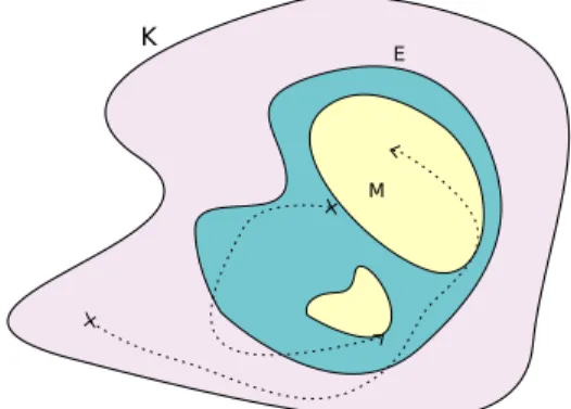
We are now ready to state LaSalle’s invariance principle, illustrated by Fig.1. Theorem 1 (LaSalle’s invariance principle). Assume F has continuous first partial derivatives and F (0) = 0. Let K be an invariant compact set. Sup-pose there is a scalar function V which has continuous first partial derivatives in K and is such that ˜V (p) 6 0 in K. Let E be the set of all points p ∈ K such that ˜V (p) = 0. Let M be the largest invariant set in E. Then for every solution y starting in K, y(t) → M as t → +∞.
K
E
M
Fig. 1. Illustration of LaSalle’s invariance principle
2.2 Relaxing Hypotheses
Some of LaSalle’s hypotheses are unnecessary, although they are justified by the context. In his paper [15], he allows himself any assumption which makes it easier to focus on the method.
First, LaSalle assumes there is an equilibrium at the origin because his method is designed to show convergence to this equilibrium. The fact that it is the origin is just a convenience allowed by an easy translation. What is more,
the existence of an equilibrium plays no role in the validity of Theorem1. Thus, we removed the hypothesis F (0) = 0.
Still regarding the vector field F , the assumption “F has continuous first partial derivatives” is also a convenience. What is truly needed, as LaSalle puts it, is “any other conditions that guarantee the existence and uniqueness of solutions and the continuity of the solutions relative to the initial conditions”. We can even go further and assume these properties only on the subset K of the ambient space. Indeed, for some systems the vector field is valid only in a restricted area, for instance when using a control function which has singularities (see e.g. [18]). Then, the ambient space does not need to be IRn, nor does it need to be a finite-dimensional vector space. A normed module over IR was sufficient to prove this result. Since we work in an abstract normed module, we cannot express ˜V using the gradient of V . However, in IRn we know that for any points p and q, the scalar product between q and the gradient of V at point p is the value of the differential of V at point p applied to q. Thus, ˜V (p) can be expressed as the differential of V at point p applied to F (p), which generalizes the definition of ˜V to normed modules.
˜
V (p) = h(grad V )(p), F (p)i = (dVp◦ F )(p)
Finally, concerning the Lyapunov function V , the assumption of continuous first partial derivatives is again a convenience. It is sufficient for V to be differen-tiable in K. Indeed, when y is a solution to (1), a step in the proof of Theorem1 is to show that V ◦ y is non increasing using the assumption ˜V (p) 6 0 in K. Remarking that
( ˜V ◦ y)(t) = (dVy(t)◦ F ◦ y)(t) = (dVy(t)◦ ˙y)(t)
so that ˜V ◦ y is the derivative of V ◦ y, only the existence of this derivative is required to conclude this step.
2.3 Strengthening the Conclusion
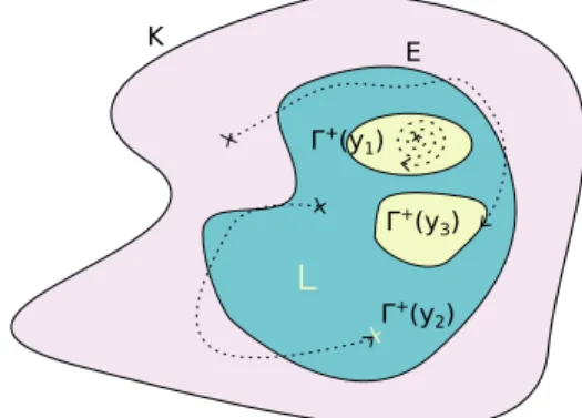
While studying LaSalle’s proof [15], we noticed it proves more than the re-sult stated by Theorem 1. Indeed, the largest invariant subset M of the set n
p ∈ K | ˜V (p) = 0owe called E is not interesting in itself: it is the fact that M is an invariant subset of E which gives M the nice property of being reduced to the equilibrium in LaSalle’s applications.
The maximality of M plays a minor role in LaSalle’s proof: given a solution y starting in K, this function happens to approach an invariant subset of E, which depends on y, as time goes to infinity, thus y approaches any of its supersets and M in particular. This set depending on y is in fact the positive limiting set of y, defined as follows:
Definition 4. Let y be a function of time. The positive limiting set of y, denoted by Γ+(y), is the set of all points p such that
In other terms, Γ+(y) is the set of limit points of y at infinity. The fact that
a function with values in a compact set approaches its limit points as time goes to infinity is intuitive and easy to prove. The fact that this set is invariant is a consequence of the continuity of solutions relative to initial conditions. The core of LaSalle’s proof is thus to show that for all solution y starting in K, we have
Γ+(y) ⊆np ∈ K | ˜V (p) = 0o.
Let us give an intuition of proof of this point. The first step is to remark that it is in fact sufficient to prove that V is constant on Γ+(y) thanks to the
interpretation of ˜V in terms of derivative. Then, the second step is to reduce this statement to the fact that V ◦ y converges at infinity. Finally, this last statement is just a consequence of the fact that V ◦ y is a bounded non increasing function. Now, to remove the dependency in y, it is sufficient to take the union of all Γ+(y) for y solution starting in K, which is still an invariant subset of E and is thus smaller than the largest of them.
Ultimately, we proved the following result, illustrated by Fig.2:
Theorem 2. Assume F is such that we have the existence and uniqueness of solutions to (1) and the continuity of solutions relative to initial conditions on an invariant compact set K. Suppose there is a scalar function V , differentiable in K, such that ˜V (p) 6 0 in K. Let E be the set of all points p ∈ K such that
˜
V (p) = 0 and L be the union of all Γ+(y) for y solution starting in K. Then, L
is an invariant subset of E and for all solution y starting in K, y(t) → L as t → +∞. K E +(y 2) +(y 1) +(y 3)
Fig. 2. Illustration of the refined version of LaSalle’s invariance principle
3
Formalization
We present in this section the notations we used to make our formalization more readable and intuitive. Then we discuss details on how we worked with
dif-ferential equations and how we expressed topological notions such as convergence and compactness.
3.1 Real Analysis and Notations
Our formalization is based on the Coquelicot library [3], which is itself compatible with Coq’s standard library on classically axiomatized real num-bers [20]. The Coquelicot library exploits the notion of filter to develop a theory of convergence. It was inspired by the work of Hölzl et al. on the analysis library of Isabelle/HOL [13].
Let us first recall some mathematical background and give some intuition. In topology, a filter is a set of sets, which is nonempty, upward closed, and closed under intersection. In this work, we use extensively two filters on real numbers: the set {N | ∃ε > 0, Bε(p) ⊆ N } of neighbourhoods of a point p and
the set of neighbourhoods of +∞ i.e. the set of sets that contain [M, +∞) for some M . The former is denoted by (locally p) in Coquelicot and the latter by (Rbar_locally p_infty). With these definitions, f converges to q at point p iff the image by f of the filter of neighbourhoods of p is a subset of the filter of neighbourhoods of q. Even though this definition unfolds to the elementary characterization of convergence ∀ε > 0, ∃δ > 0, ∀r, |r − p| < δ ⇒ |f (r) − q| < ε, keeping the abstraction in terms of filters as much as possible yields more concise proofs and is also well supported by the library.
In this work, we experimented with notations to overload the ones in Co-quelicot, so that they read a bit closer to textbook mathematics. First, since sets are represented as predicates over a type, we pose set T := T -> Prop
and we define Mathematical Components-like notations to denote set the-oretic operations. Indeed set0, setT and [set p] are respectively the empty set, the total set and the singleton {p}. Also, (A ‘&‘ B), (A ‘|‘ B), (~‘ A) and (A ‘\‘ B) are respectively the intersection, union, complement and dif-ference. We write (A ‘<=‘ B) for A ⊆ B and (A !=set0) for ∃p ∈ A, note that !=set0 is a token here. We also introduce set comprehension notations [set p | A p] (which is a typed alias for (fun p => A)) and the big opera-tors \bigcup_(i in A) F i and \bigcap_(i in A) F i respectively denoting union and intersection of families indexed by A.
Secondly, Coquelicot introduces layers over filters to abbreviate conver-gence. For example the predicate (is_lim f t p) is specialized to t and p in Rbar (i.e. IR ∪ {±∞}) and is defined in terms of filterlim which expands to the definition of this section. Since we introduce other notions of convergence in Sect.3.3, adding more alternative definitions for approximately the same notion would only clutter the formalization, so we decided to remove this extra-layer. Instead, we provide a unique mechanism to infer which notion of convergence is required, by inspecting the form of the arguments and their types.
We now write f @ p --> q whatever the types of p and q: our mechanism selects the appropriate filters for p and q. This is in fact the composition of two independent notations: f @ p selects a filter for p and applies f to it, while q’ --> q selects filters for q’ and q and compares them.
We provide the notation +oo for the element p_infty of Rbar, so that a limit p of f at +∞ now reads f @ +oo --> p. Moreover, although we do not use it in this part of the development, we also cast functions from nat, i.e. sequences, to the only sensible filter on nat (named eventually in Coquelicot), so that one can write u --> p where u : nat -> U is a sequence.
Coq’s coercion mechanism is not powerful enough to handle casts from an arbitrary term to an appropriate filter. Hence, the mechanism to automatically infer a filter from an arbitrary term and its type is implemented using canonical structures. More precisely, we provide three structures: the first one to recognize terms that could be cast to filters, the second one to recognize types whose elements could be cast to filters, and the third one to recognize arrow types which could be cast to filters. If the first canonical structure fails to cast a given term to a filter, it gives its type to the second canonical structure and if it is an arrow it tries to match the source of the arrow using the third canonical structure.
3.2 On Differential Equations
To deal with systems of differential equations, we also use the Coquelicot library [3], which already contains convenient definitions for functional analysis. This library also contains a hierarchy of topological structures, among which is the structure of normed module we used for the ambient space.
The property of being a solution to the differential system (1) is then easily expressed as follows: y is a solution if at each time t, the derivative of y at point t is (F ◦ y)(t). In Coq:
Definition is_sol (y : R -> U) :=
forall t, is_derive y t (F (y t)).
Here, U is the ambient space and R the set of real numbers. We could have considered only non negative times, since our goal is to describe physical systems. However, for reasons we will give later, we stick to this more constrained version in this paper.
Now, what we need is a way to express the existence and uniqueness of solutions to (1) and the continuity of solutions relative to initial conditions. In our work, we assumed the existence of a function sol : U -> R -> U which represents all the solutions to (1). Its first argument corresponds to the initial condition and the second one to time. Thus, when time is equal to 0, the result of this function must be equal to the initial condition.
Hypothesis sol0 : forall p, sol p 0 = p.
We combined the conditions of existence (for all p in K, sol p is a solution) and uniqueness of solutions into the following hypothesis: a function y starting in K is a solution to (1) if and only if it is equal to the function sol (y 0), that is the solution which has same initial condition.
Note that here we wrote an equality between functions. This assumption to-gether with the axiom of functional extensionality made our proofs more natural and shorter. Indeed, by using solP we can replace any solution by an application of the function sol, which removes all the hypotheses of the form is_sol y from our theorems. Moreover, proof scripts in the SSReflect tactic language [11] heavily rely on the rewriting of equalities.
This hypothesis would not be satisfiable if, as mentioned before, we con-strained the derivative of solutions only for non negative times. Indeed, we could not control the values of these solutions for negative times, hence there would be (infinitely) many solutions y different from sol (y 0). Adapting naively this hypothesis by considering equality only on non negative times would cancel all the benefits of this formulation.
One solution could be to change the type of the functions in order to work with functions whose domain is the set of non negative real numbers. This would require to construct the type for this set and to develop its theory. A compromise which would be easier to implement and more ligthweight in our context is to keep functions on IR, but only require the solution to satisfy the differential equation for non negative times, and fix its value for negative times. For example we could ask the function to be constant equal to y(0) for negative values, or make the solution symmetric with regard to its initial value (i.e. y(−t) = 2y(0) − y(t)), which would keep the solution derivable everywhere.
Finally, the continuity of solutions relative to initial conditions on K is ex-pressed as the continuity on K of the functionfun p : U => sol p t for all t. 3.3 Convergence to a Set
To generalize the notion of convergence to a point to convergence to a set, what we called “approaching a set when time goes to infinity” in Sect.2, we need to generalize the notion of neighbourhood filter to a set. Recall the definition of neighbourhood filter for a point (Sect. 3.1): a neighbourhood of a point is a set that contains a ball with positive radius centered on this point. In Co-quelicot [3], this definition is not restricted to real numbers but applies to any uniform space.
Definition locally (p : U) :=
[set A | exists eps : posreal, ball p eps ‘<=‘ A].
For a set, there is no ball anymore. However, we can extend the set with a band of fixed width ε, which is in fact the union of all balls of radius ε centered on points of the set.
Definition ball_set (A : set U) (eps : posreal) := \bigcup_(p in A) ball p eps.
The neighbourhood filter for a set then has a very analogous definition to the one of neighbourhood filter for a point.
Definition locally_set (A : set U) :=
[set B | exists eps : posreal, ball_set A eps ‘<=‘ B].
Instance locally_set_filter (A : set U) : Filter (locally_set A).
We can prove that it is a generalization of the notion of neighbourhood filter for a point by proving that we define the same filter on the singleton [set p] as with Coquelicot’s definition on p.
Lemma locally_set1P p A : locally p A <-> locally_set [set p] A. In our notation mechanism from Sect. 3.1, we declare locally_set to be the canonical filter to use for sets over a uniform space, so that we can write y @ +oo --> A where A is a set. Thus, the notion of convergence to a set is expressed thanks to Coquelicot’s notion of limit using this particular filter. And again, we can prove that it generalizes Coquelicot’s notion of limit when applied on singletons.
Lemma cvg_to_set1P y p : y @ +oo --> [set p] <-> y @ +oo --> p.
3.4 Compactness
To express compactness, we decided to experiment with a definition of com-pact sets using filters. In fact, this definition involves the notion of clustering, which is closely related to convergence and limit points. Indeed, a filter clusters to a point if each of its elements intersects each neighbourhood of the point. We say that a filter clusters if there is a point to which it clusters.
Definition cluster (F : set (set U)) p :=
forall A B, F A -> locally p B -> A :&: B !=set0
To see the link with limit points of a function y, consider the filter (y @ +oo), which is the set of sets which ultimately contain all images of y (formerly filtermap y (Rbar_locally p_infty) in Coquelicot). The set of points to which (y @ +oo) clusters is exactly the positive limiting set of y i.e. the set of limit points of y (recall Definition4).
Definition pos_limit_set (y : R -> U) :=
\bigcap_(eps : posreal) \bigcap_(T : posreal) [set p | Rlt T ‘&‘ (y @^-1‘ ball p eps) !=set0].
Lemma plim_set_cluster (y : R -> U) : pos_limit_set y = cluster (y @ +oo).
Note that we wrote an equality between sets i.e. between functions with propositions as value. We used the axiom of propositional extensionality (on top of functional extensionality) to be able to prove this. Again, this makes our code closer to textbook mathematics.
We were already using this equality to prove some properties of the positive limiting set of a function y. Consequently, we decided to state each property
of this set as a property of cluster (y @ +oo). Thanks to this strategy, we managed to shorten some of our proofs.
A set A is compact if every proper filter on A clusters in A.
Definition compact A :=
forall (F : set (set U)), F A -> ProperFilter F -> (A :&: cluster F) !=set0.
Note how the hypothesis “on A” has been translated into “A is an element of F”. This is possible thanks to the properties of filters: every filter on A is a filter base in U whose completion is a filter containing A, and every filter on U containing A defines a filter on A when restricted to sets contained in A. Thanks to this, we do not have to consider the subspace topology, which would add complications. Indeed, the type classes Filter and ProperFilter of Coquelicot are defined on sets of sets in a uniform space i.e. on functions of type (U -> Prop) -> Prop
for U a uniform space. The UniformSpace structure of Coquelicot requires an element of typeType, while in our context A is of type U -> Prop. Canonically transfering structures to subsets would then require wrapping functions into types, while our solution is simpler.
This notion of compact set is quite convenient to use to work with conver-gence and limit points: the only hard part is finding the right filter on your compact set and then the cluster point this hypothesis gives you is usually the point your are looking for. However for other proofs this notion is quite com-plicated to use. Proving that a set is compact requires finding a cluster point for any abstract proper filter on this set, or going through a proof by contradic-tion. Moreover, to prove that any compact set is bounded, we had to go through the definition of compactness based on open covers. We proved the equivalence between both definitions following the proof in Wilansky’s textbook on topol-ogy [24] (see Sect.5for more details on the proof).
4
The Formal Statement of LaSalle’s Invariance Principle
As explained in Sect.2, we formalized a slightly stronger version of LaSalle’s invariance principle [15]. In particular, we proved the convergence of solutions to (1) to a more constrained set: the union of the positive limiting sets of the solutions starting in K.
Definition limS (A : set U) :=
\bigcup_(q in A) cluster (sol q @ +oo).
Recall that we require K to be compact and invariant (see Definition2). Both these hypotheses are used to prove the convergence of solutions to limS K.
Definition is_invariant A :=
forall p, A p -> forall t, 0 <= t -> A (sol p t).
Lemma cvg_to_limS (A : set U) : compact A -> is_invariant A ->
This is in fact an “easy” part of LaSalle’s invariance principle. It is indeed sufficient for a function to ultimately have values in a compact set in order for it to converge to the set of its limit points, hence to any superset of its positive limiting set.
Lemma cvg_to_pos_limit_set y (A : set U) :
(y @ +oo) A -> compact A -> y @ +oo --> cluster (y @ +oo).
Lemma cvg_to_superset A B y : A ‘<=‘ B -> y @ +oo --> A -> y @ +oo --> B.
The invariance of K is a strong way to force the solutions to ultimately have values in K. However, since in our proof of LaSalle’s invariance principle we need to use the uniqueness of solutions for initial conditions which are values of solutions starting in K, the invariance of K is required anyway.
There are two other aspects to our version of LaSalle’s invariance principle: limS K is invariant and it is a subset of the set of points p for which ˜V(p) = 0. The first point does not need any hypothesis: the positive limiting set of any solution starting in K is invariant, hence any union of such sets is invariant too.
Lemma invariant_pos_limit_set p :
K p -> is_invariant (cluster (sol p @ +oo)).
Lemma invariant_limS A : A ‘<=‘ K -> is_invariant (limS A).
As explained in Sect.2.3, the core of LaSalle’s proof is thus the second point. To state this part, we need to use the differential of the Lyapunov function V. Indeed, as mentioned in Sect.2.2, since we work in an abstract normed module, we cannot express ˜V using the gradient of V. We express differentials using Co-quelicot [3]: filterdiff f (locally p) g expresses the fact that g is the dif-ferential of f at point p. Thus, we assume a function V’ : U -> U -> R which is total, together with the hypothesis that for any p in K, V’ p is the differential of V at point p (i.e.forall p : U, K p -> filterdiff V (locally p) (V’ p)). All hypotheses on ˜V can then be expressed by replacing it with the function
fun p => (V’ p \o F) p.
Assuming a total function V’ is a way to mimic Coquelicot’s proof style on derivatives. Indeed, to represent the derivative of a real function f : R -> R in Coquelicot, one has access to a total function Derive f. All theorems then concern Derive f, with the hypothesis that f admits a derivative at some point x, written ex_derive f x, when it is needed. This is a very convenient way to deal with derivatives. However, because Coquelicot lacks such a total function for differentials, we had to introduce the differential as a parameter.
Finally, the last part of our version of LaSalle’s invariance principle, i.e. the set limS K is a subset of the set of points p for which ˜V(p) = 0, is stated as follows:
Lemma stable_limS (V : U -> R) (V’ : U -> U -> R) :
(forall p : U, K p -> filterdiff V (locally p) (V’ p)) -> (forall p : U, K p -> (V’ p \o F) p <= 0) ->
Note that the proof in Coq follows exactly the same steps as in the paper proof we sketched in Sect.2.3.
5
On Classical Reasoning
Several proofs in our work required classical reasoning, although we tried to remain as constructive as possible. Indeed, while proofs and statements in constructive analysis are very different from the ones in classical analysis, we believe some of our constructive proofs could still be used in a purely constructive context. In particular, in our development we use a classical axiomatization of real numbers, but we hope some results are actually independent from the representation of real numbers. For example, most results in topology, like our constructive theorems on sets, filters, closures, and compactness are phrased in a way which does not make real numbers appear.
Hence, we redefined some notions, namely closed sets, closures, compactness and Hausdorff separation, to fit our purposes, and the proofs that these are equivalent to preexisting definitions were often classical. We also list here two other main theorems for which we could only give a classical proof.
First, the notion of closure was very practical to use whenever closed sets appeared. In Coquelicot [3], a set A is closed if it contains all points for which the complement of A is not a neighbourhood. A point is in the closure of a set if all its neighbourhoods intersect the set. A set is closed if and only if its closure is included in it (the other inclusion always holds).
Definition closed (A : set U) :=
forall p, ~ (locally p (~‘ A)) -> A p.
Definition closure (A : set U) p :=
forall B, locally p B -> A ‘&‘ B !=set0.
Lemma closedP (A : set U) : closed A <-> closure A ‘<=‘ A.
The right implication of closedP was proved constructively while the other direction required classical reasoning. The notion of closure proved to be very practical, especially in our settings since it is related to clustering: a filter clusters to a point if and only if this point is in the closure of each element of the filter.
Lemma clusterE F : cluster F = \bigcap_(A in F) (closure A). Then, the proof of equivalence between the filter-based and open covers-based definitions of compactness is classical. In fact, we prove this equivalence by going through a third definition of compactness: a set A is compact if every family of closed sets of A with the finite intersection property has a nonempty intersection. This definition is very close to the filter-based one, and we proved constructively that they are equivalent. Indeed, the set of all finite intersections in such a family is a filter base defining a proper filter which clusters. Conversely, the family of closures of the elements of a proper filter which clusters has the finite intersection property. It is the equivalence between this third definition and the open covers-based definition which is classical. More precisely, both directions
in this equivalence are proved by contraposition and classical steps are required to push negations under existential quantifiers and to remove double negations. Similarly, we worked with a different definition of a Hausdorff space. We proved that normed modules are necessarily Hausdorff spaces. This allowed us to prove that the compact set K is also closed, which was needed to show that the positive limiting set of any solution starting in K is included in K. We could have used the usual notion of Hausdorff space (whenever you have two different points, you can find two respective neighbourhoods of these points which do not intersect), but in fact, its contrapositive was more practical in our settings because it admits a nice statement using clustering: if two points p and q are such that all their neighbourhoods intersects, i.e. the neighbourhood filter of p clusters to q (and vice-versa), then they are equal.
Definition hausdorff (U : UniformSpace) :=
forall p q : U, cluster (locally p) q -> p = q.
Lemma hausdorffP (U : UniformSpace) :
hausdorff U <-> forall p q : U, p <> q -> exists A B, locally p A /\ locally q B /\ forall r, ~ (A ‘&‘ B) r.
Again, the proof of equivalence between both definitions required classical reasoning to push and remove negations.
Another classical proof we did is the proof of convergence of a function with values ultimately in a compact set to its positive limiting set.
Lemma cvg_to_pos_limit_set y (A : set U) :
(y @ +oo) A -> compact A -> y @ +oo --> cluster (y @ +oo). We proved this theorem in two ways. The first proof is by contradiction, as in LaSalle’s paper [15]. The second one goes through a generalization of this result: any proper filter on a compact set contains any neighbourhood of its set of cluster points.
Lemma filter_cluster (F : set (set U)) (A : set U) : ProperFilter F -> F A -> compact A ->
forall eps : posreal, F (ball_set (cluster F) eps).
We proved this lemma using yet another definition of compactness: the con-trapositive of the definition based on families of closed sets. Going back and forth between emptiness and nonemptiness properties once again introduced classical reasoning steps. Similarly, as mentioned in Sect. 3.4, we had to use a classical equivalence between two definitions of compactness to prove that compact sets are bounded.
Finally, we had to prove classically that a monotonic bounded real func-tion admits a finite limit at infinity. For instance in the case of a non decreas-ing function, one has to prove that the lowest upper bound of its values is the aforementioned limit. What is classical is the proof that, if l is the least upper bound of the set A, then for all ε > 0 there exists p ∈ A such that l − ε 6 p 6 l. This last example illustrates the problem, already noticed by A. Mahboubi and G. Melquiond, that Coq’s axiomatization of real numbers
is not expressive enough to give an arbitrary approximation of a least upper bound.
6
Related Work
Several formalizations in topology already exist: in Coq [4], in PVS [16], in Isabelle/HOL [13] or in Mizar [7,22] for instance. All of them express compactness using open covers. We adapted Cano’s formalization [4] for our proof of equivalence with the filter-based definition. We could not use it directly since it relies on the eqType structure of the Mathematical Components library and Coquelicot’s structures [3] are not based on this structure.
Note that in the work of Hölzl et al. [13] there is a definition of compactness in terms of filters which is slightly different from ours: a set A is compact if for each proper filter on A there is a point p ∈ A such that a neighbourhood of p is contained in the filter. This is a bit less convenient to use than clustering since you cannot choose the neighbourhood. To our knowledge, our work is the first attempt to exploit the filter-based definition of compactness to get simple proofs on convergence.
We must also mention Coquelicot’s definition of compactness, which is based on gauge functions, and Coq’s topology library by Schepler3. Both are
unfortunately unusable in our context: Coquelicot’s definition is specialized to IRn while we are working on an abstract normed module, and Schepler’s library does not interface with Coquelicot, since it redefines filters for in-stance. Schepler’s library contains a proof of equivalence between the filter-based and open covers-based definitions of compactness, which is very close to ours. However, these definitions concern topological spaces whereas, as mentionned in Sect.3.4, we focus on subsets of such spaces without referring to the subspace topology.
Concerning formalizations on stability and Lyapunov functions, Chan et al. [5] used a Lyapunov function to prove in Coq the stability of a particular system. They have however no proof of a general stability theorem. Mitra and Chandy [21] formalized in PVS stability theorems using Lyapunov-like functions in the particular case of automata. Herencia-Zapana et al. [12] took another ap-proach to stability proofs: stability proofs using Lyapunov functions, under the form of Hoare triples annotations on C code, are used to generate proof obliga-tions for PVS.
We are definitely not the first to generalize LaSalle’s invariance principle. We decided to prove a version of the principle which is close to the original statement but several generalizations were designed to make it available in more complex settings. Chellaboina et al. [6] weakened further the regularity hypoth-esis on the Lyapunov function at the cost of sign conditions and a boundedness hypothesis on the Lyapunov function along the trajectories. Barkana et al. [1] restricted the hypotheses on the Lyapunov function to hypotheses along the tra-jectories in order to generalize LaSalle’s invariance principle to nonautonomous
3
systems. Mancilla-Aguilar and García [19] generalized LaSalle’s invariance prin-ciple to switched autonomous systems by adding further conditions related to the switching, but removed the conditions of existence and uniqueness of solu-tions and of continuity of the solusolu-tions relative to initial condisolu-tions by working on a set of admissible trajectories. Fischer et al. [8] also weakened the hypotheses on the solutions of a nonautonomous system by using a generalized notion of solution.
7
Conclusion and Future Work
In this paper we presented our formalization of LaSalle’s invariance principle, a theorem about the asymptotic stability of solutions to a nonlinear system of differential equations. We proved a version of this theorem which is very close to its original statement but we removed unnecessary hypotheses and chose a more precise conclusion.
Our use of set theoretic notations in this formalization made our proofs more readable, closer to the intuition of filters as sets of sets. Functional extensionality also gave us a convenient way to write proofs on the solutions to a differential equation, allowing us to use a single function to represent all of them. We used propositional extensionality to be able to prove equalities between sets, but it is not as critical as functional extensionality: all the proofs were written without this axiom before we decided to add it.
Our experiment with filter-based compactness is partially conclusive: filters are really adapted to proofs on convergence but we had to use other definitions of compactness for other purposes.
All in all, our formalization of LaSalle’s invariance principle takes around 1250 lines. Around 250 lines were devoted to the proofs of the properties on the positive limiting set and of LaSalle’s invariance principle. The remaining 1000 lines contain the definitions of notations, the generalization of convergence no-tions to sets and proofs about closed sets, compact sets and monotonic funcno-tions. This formalization is a step towards a formal verification of dynamical sys-tems. LaSalle’s invariance principle and its extensions play an important role in the study of control techniques. We plan to use this work to formally verify a control law for the swing-up of an inverted pendulum [18].
Acknowledgements
References
1. Barkana, I.: Defending the beauty of the Invariance Principle. Int. J. Control 87(1), 186–206 (2014),http://dx.doi.org/10.1080/00207179.2013.826385
2. Blazy, S., Paulin-Mohring, C., Pichardie, D. (eds.): Interactive Theorem Prov-ing - 4th International Conference, ITP 2013, Rennes, France, July 22-26, 2013. Proceedings, Lecture Notes in Computer Science, vol. 7998. Springer (2013),
http://dx.doi.org/10.1007/978-3-642-39634-2
3. Boldo, S., Lelay, C., Melquiond, G.: Coquelicot: A User-Friendly Library of Real Analysis for Coq. Mathematics in Computer Science 9(1), 41–62 (2015), http: //dx.doi.org/10.1007/s11786-014-0181-1
4. Cano, G.: Interaction entre algèbre linéaire et analyse en formalisation des math-ématiques. (Interaction between linear algebra and analysis in formal mathemat-ics). Ph.D. thesis, University of Nice Sophia Antipolis, France (2014), https: //tel.archives-ouvertes.fr/tel-00986283
5. Chan, M., Ricketts, D., Lerner, S., Malecha, G.: Formal Verification of Stability Properties of Cyber-physical Systems (Jan 2016)
6. Chellaboina, V., Leonessa, A., Haddad, W.M.: Generalized Lyapunov and invari-ant set theorems for nonlinear dynamical systems. Systems & Control Letters 38(4–5), 289 – 295 (1999), http://www.sciencedirect.com/science/article/ pii/S0167691199000766
7. Darmochwał, A.: Compact Spaces. Formalized Mathematics 1(2), 383–386 (1990),
http://fm.mizar.org/1990-1/pdf1-2/compts_1.pdf
8. Fischer, N.R., Kamalapurkar, R., Dixon, W.E.: LaSalle-Yoshizawa Corollaries for Nonsmooth Systems. IEEE Trans. Automat. Contr. 58(9), 2333–2338 (2013),http: //dx.doi.org/10.1109/TAC.2013.2246900
9. Gonthier, G.: Formal proof – The Four-Color Theorem. Notices of the AMS 55(11), 1382–1393 (2008)
10. Gonthier, G., Asperti, A., Avigad, J., Bertot, Y., Cohen, C., Garillot, F., Roux, S.L., Mahboubi, A., O’Connor, R., Biha, S.O., Pasca, I., Rideau, L., Solovyev, A., Tassi, E., Théry, L.: A Machine-Checked Proof of the Odd Order Theorem. In: Blazy et al. [2], pp. 163–179,http://dx.doi.org/10.1007/978-3-642-39634-2_ 14
11. Gonthier, G., Mahboubi, A., Tassi, E.: A Small Scale Reflection Extension for the Coq system. Research Report RR-6455, Inria Saclay Ile de France (2015),
https://hal.inria.fr/inria-00258384
12. Herencia-Zapana, H., Jobredeaux, R., Owre, S., Garoche, P., Feron, E., Pérez, G., Ascariz, P.: PVS linear algebra libraries for verification of control software algorithms in C/ACSL. In: Goodloe, A., Person, S. (eds.) NASA Formal Methods - 4th International Symposium, NFM 2012, Norfolk, VA, USA, April 3-5, 2012. Proceedings. Lecture Notes in Computer Science, vol. 7226, pp. 147–161. Springer (2012),http://dx.doi.org/10.1007/978-3-642-28891-3_15
13. Hölzl, J., Immler, F., Huffman, B.: Type Classes and Filters for Mathematical Analysis in Isabelle/HOL. In: Blazy et al. [2], pp. 279–294, http://dx.doi.org/ 10.1007/978-3-642-39634-2_21
14. Khalil, H.: Nonlinear Systems. Pearson Education, Prentice Hall (2002), https: //books.google.fr/books?id=t_d1QgAACAAJ
15. LaSalle, J.: Some Extensions of Liapunov’s Second Method. IRE Transactions on Circuit Theory 7(4), 520–527 (Dec 1960)
16. Lester, D.R.: Topology in PVS: Continuous Mathematics with Applications. In: Proceedings of the Second Workshop on Automated Formal Methods. pp. 11– 20. AFM ’07, ACM, New York, NY, USA (2007),http://doi.acm.org/10.1145/ 1345169.1345171
17. Liapounoff, A.: Problème général de la stabilité du mouvement. Annales de la Faculté des sciences de Toulouse : Mathématiques 9, 203–474 (1907), http:// eudml.org/doc/72801
18. Lozano, R., Fantoni, I., Block, D.: Stabilization of the inverted pendulum around its homoclinic orbit. Systems & Control Letters 40(3), 197–204 (2000)
19. Mancilla-Aguilar, J.L., García, R.A.: An extension of LaSalle’s invariance principle for switched systems. Systems & Control Letters 55(5), 376–384 (2006), http: //dx.doi.org/10.1016/j.sysconle.2005.07.009
20. Mayero, M.: Formalisation et automatisation de preuves en analyses réelle et numérique. Ph.D. thesis, Université Paris VI (décembre 2001)
21. Mitra, S., Chandy, K.M.: A Formalized Theory for Verifying Stability and Con-vergence of Automata in PVS. In: Mohamed, O.A., Muñoz, C.A., Tahar, S. (eds.) Theorem Proving in Higher Order Logics, 21st International Conference, TPHOLs 2008, Montreal, Canada, August 18-21, 2008. Proceedings. Lecture Notes in Com-puter Science, vol. 5170, pp. 230–245. Springer (2008), http://dx.doi.org/10. 1007/978-3-540-71067-7_20
22. Padlewska, B., Darmochwał, A.: Topological Spaces and Continuous Functions. Formalized Mathematics 1(1), 223–230 (1990), http://fm.mizar.org/1990-1/ pdf1-1/pre_topc.pdf
23. The Coq Development Team: The Coq proof assistant reference manual (2016),
http://coq.inria.fr, version 8.6
24. Wilansky, A.: Topology for Analysis. Dover books on mathematics, Dover Publ., New York, NY (2008),http://cds.cern.ch/record/2222525