HAL Id: hal-01783580
https://hal.archives-ouvertes.fr/hal-01783580
Submitted on 14 Jan 2019HAL is a multi-disciplinary open access archive for the deposit and dissemination of sci-entific research documents, whether they are pub-lished or not. The documents may come from teaching and research institutions in France or abroad, or from public or private research centers.
L’archive ouverte pluridisciplinaire HAL, est destinée au dépôt et à la diffusion de documents scientifiques de niveau recherche, publiés ou non, émanant des établissements d’enseignement et de recherche français ou étrangers, des laboratoires publics ou privés.
LOPC in coastal waters
B. Espinasse, S. Basedow, L. Berline, S. Schultes, M. Zhou, F Carlotti
To cite this version:
B. Espinasse, S. Basedow, L. Berline, S. Schultes, M. Zhou, et al.. Conditions for assessing zooplankton abundance with LOPC in coastal waters. Progress in Oceanography, Elsevier, 2018, 163, pp.260-270. �10.1016/j.pocean.2017.10.012�. �hal-01783580�
Manuscript number PROOCE_2017_45_R2
Title Conditions for assessing zooplankton abundance with LOPC in coastal waters. Article type Full Length Article
Abstract
Recent technical advances in laser-based systems to measure zooplankton distribution have opened new perspectives in ecological and behavioral studies by significantly improving the horizontal and vertical sampling resolution, providing information on zooplankton patchiness and on the influence of small scale physical processes. The application of laser-based systems also led to new challenges on the identification of organisms vs. particulate matter. In areas with high detritus abundances, zooplankton abundances might be overestimated by counting plankton and detritus together. We investigated the contribution of detritus in Laser Optical Plankton Counter (LOPC) data collected during two cruises on the continental shelf of the Gulf of Lion (NW Mediterranean Sea). The study area was characterized by several types of ecoregions owing to the influence of winds, freshwater runoff and intrusion of oligotrophic waters from offshore. We identified the main mechanisms leading to the formation of detritus as a function of environmental conditions and developed a method to assess the contribution of detritus in LOPC counts based on the proportion of large particles (multi-element plankton, MEPs). Highest percentages of detritus (up to 90 % of the counts, mainly particulate organic matter from various sources) were found in stratified conditions associated with relatively high chlorophyll a concentration (chl-a; ca 2 mg m-3). Discontinuities in density profiles alone also resulted in peaks of particles concentrations. We suggested a threshold of 2 % of MEPs in LOPC counts above which the LOPC is most likely counting more detritus than organisms. This easy check of the detritus contribution to total LOPC counts was applied to datasets from different marine ecological situations (glacial input, clear water, productive shelf) and gave successful results in different biogeographical regions (e.g. high latitude and tropical habitats).
Keywords laser-based sensors; ZooScan; stratification; thin layers; aggregates Manuscript category Biological Oceanography
Corresponding Author Boris Espinasse Corresponding Author's
Institution
University of British Columbia
Order of Authors Boris Espinasse, Sünnje Basedow, Sabine Schultes, Meng Zhou, Léo Berline, Francois Carlotti
Suggested reviewers Kohei Matsuno, Pieter Vandromme, Marc Hufnagl, Jason Everett
Submission Files Included in this PDF File Name [File Type]
cover letter rev.docx [Cover Letter]
Responses LOPC ms_R1.docx [Response to Reviewers] Highlights.docx [Highlights]
LOPC-ms-R1.docx [Manuscript File] Fig_LOPC_new.docx [Figure] Tables.docx [Table]
To view all the submission files, including those not included in the PDF, click on the manuscript title on your EVISE Homepage, then click 'Download zip file'.
A new method to interpret LOPC counts was developed.
The environmental conditions and the mechanisms resulting in detritus formation were identified.
LOPC derived indicators were used successfully to determine the contribution of detritus in total counts.
Thresholds for these LOPC indicators are used to define different situations with varying contribution of detritus.
1
1 Conditions for assessing zooplankton abundance with LOPC in coastal waters. 2
3
4 Authors:
5 Espinasse B.*, 1, 2, 3, Basedow S.4, Schultes S.5, Zhou M.6, Berline L.1 and Carlotti F.1
6 7 8 9
10 1Aix Marseille Université, CNRS/INSU, IRD, Mediterranean Institute of Oceanography (MIO),
11 UM 110, Marseille, France
12
13 2Faculty of Biosciences and Aquaculture, Nord University, N-8049 Bodø, Norway
14
15 3Department of Earth, Ocean, and Atmospheric Sciences, University of British Columbia, 2207
16 Main Mall, Vancouver, British Columbia, Canada V6T 1Z4
17 4Faculty of Biosciences, Fisheries and Economics, UiT The Arctic University of Norway, N-9037
18 Tromsø
19
20 5Aquatic Ecology Group, Ludwig Maximilian University of Munich (LMU), Grosshadernerstr. 2,
21 82152 Planegg-Martinsried
22
23 6Shanghai Jiao Tong University, Institute of Oceanology, 800 Dongchuan Rd, Minhang, Shanghai,
24 China, 200240 25 26 27 28 29 30 31 ______________________
32 *Corresponding author: bespinasse@eoas.ubc.ca
3 4 5 6 7 8 9 10 11 12 13 14 15 16 17 18 19 20 21 22 23 24 25 26 27 28 29 30 31 32 33 34 35 36 37 38 39 40 41 42 43 44 45 46 47 48 49 50 51 52 53 54 55
2 33 Abstract
34 Recent technical advances in laser-based systems to measure zooplankton distribution have opened
35 new perspectives in ecological and behavioral studies by significantly improving the horizontal
36 and vertical sampling resolution, providing information on zooplankton patchiness and on the
37 influence of small scale physical processes. The application of laser-based systems also led to new
38 challenges on the identification of organisms vs. particulate matter. In areas with high detritus
39 abundances, zooplankton abundances might be overestimated by counting plankton and detritus
40 together. We investigated the contribution of detritus in Laser Optical Plankton Counter (LOPC)
41 data collected during two cruises on the continental shelf of the Gulf of Lion (NW Mediterranean
42 Sea). The study area was characterized by several types of ecoregions owing to the influence of
43 winds, freshwater runoff and intrusion of oligotrophic waters from offshore. We identified the main
44 mechanisms leading to the formation of detritus as a function of environmental conditions and
45 developed a method to assess the contribution of detritus in LOPC counts based on the proportion
46 of large particles (multi-element plankton, MEPs). Highest percentages of detritus (up to 90 % of
47 the counts, mainly particulate organic matter from various sources) were found in stratified
48 conditions associated with relatively high chlorophyll a concentration (chl-a; ca 2 mg m-3).
49 Discontinuities in density profiles alone also resulted in peaks of particles concentrations. We
50 suggested a threshold of 2 % of MEPs in LOPC counts above which the LOPC is most likely
51 counting more detritus than organisms. This easy check of the detritus contribution to total LOPC
52 counts was applied to datasets from different marine ecological situations (glacial input, clear
53 water, productive shelf) and gave successful results in different biogeographical regions (e.g. high
54 latitude and tropical habitats).
55 56
57 Key words: laser-based sensors, ZooScan, stratification, thin layers, aggregates
59 60 61 62 63 64 65 66 67 68 69 70 71 72 73 74 75 76 77 78 79 80 81 82 83 84 85 86 87 88 89 90 91 92 93 94 95 96 97 98 99 100 101 102 103 104 105 106 107 108 109 110
3 58 1. Introduction
59 Owing to the high variability of physical processes at small scales and their impacts on biological
60 processes, it is necessary to sample plankton at high resolutions for resolving community structure
61 and dynamics. This issue is particularly critical in coastal areas which are the place of nursery and
62 feeding area of many fish, and recent programs such as the MERMEX project (Marine Ecosystems
63 Response in the Mediterranean Experiment; Mermex Group, 2011) called for better evaluation of
64 the pelagic fish habitats in productive coastal areas. Based on optical technologies, several optical
65 sensors have been developed in the recent years for high resolution sampling (Benfield et al., 2007).
66 The in-situ sensors are generally based on imaging technologies with relatively low image
67 resolution (e.g. Video Plankton Recorder, Underwater Video Profiler) or based on the transmission
68 or scattering of a laser beam (e.g. Laser Optical Plankton Counter, Laser In-Situ Scattering and
69 Transmissometry). These optical systems not only provide fine resolution vertical profiles but can
70 also sense fragile particles that are generally destroyed when sampling with a net (González-Quirós
71 and Checkley, 2006). Laboratory sensors are mainly based on the high resolution imaging of
72 samples collected with a net or bottles (e.g. FlowCam, ZooScan). Image-based systems allow for
73 the taxonomic identification of organisms up to a certain degree, while the laser-based systems
74 mainly provide sizes and abundances of the organisms studied. The newly developed holographic
75 technology is an exception, but is more similar to in-situ microscopes facing challenges of sampling
76 volume and data processing (Davies et al., 2011; Talapatra et al., 2013). Laser-based systems
77 measure particles in a wide range of sizes and at high frequency but do not allow to distinguish
78 between organisms and particulate matter. The contribution of detritus to counts can be significant
79 in highly productive regions such as fronts, estuarine systems or upwelling areas, so that the size
80 structure of the plankton community cannot be estimated by abundances derived from in-situ
laser-81 based sensors (Zhang et al., 2000; Ohman et al., 2012; Schultes et al., 2013; Basedow et al., 2014;
115 116 117 118 119 120 121 122 123 124 125 126 127 128 129 130 131 132 133 134 135 136 137 138 139 140 141 142 143 144 145 146 147 148 149 150 151 152 153 154 155 156 157 158 159 160 161 162 163 164 165 166 167
4
82 Trudnowska et al., 2014). Therefore, in studies focusing on the living part of the spectrum, it is
83 necessary to estimate the proportion of detritus in the total particle pool.
84 The Laser Optical Plankton Counter (LOPC, Rolls-Royce, England) measures particles and
85 mesozooplankton organisms of sizes between 100 μm and about 3 cm equivalent spherical diameter
86 (ESD) (Herman et al., 2004). It can continuously profile along transects when it is mounted on
87 profiling systems (MVP, profiling float, Acrobats etc., see for example Ohman et al., 2012;
88 Checkley et al., 2008), or can sample vertical profiles when fixed on a net frame or a rosette cage.
89 When particles pass through the tunnel and cross the laser beam, the attenuation of the light
90 intensity is measured by one or several of the 35 photodiode elements, each with 1 mm width. The
91 digital size of a particle is inferred from the intensity changes in shadowed elements, which is
92 converted to ESD. If a particle is recorded by at least 3 diode elements, it will be considered as a
93 multi-element plankton (MEP), in contrast to single element plankton (SEP). In addition to the
94 ESD, more information about the MEPs is provided by the LOPC, allowing to compute an
95 attenuance index (AI). This index has been successfully used to separate detritus and living
96 organisms when targeting large-sized copepods (> 1.5 mm ESD) based on their opacity (Checkley
97 et al., 2008; Gaardsted et al., 2010). For the SEPs, which constitute the dominant part of LOPC
98 counts in the smaller size ranges, no additional information on the transparency of particles is
99 provided, making a direct separation of organisms and detritus impossible. Lately, methods to
100 separate organisms and detritus were proposed, either based on the lognormal distribution expected
101 for size spectra of non-living particles (Petrik et al., 2013; Marcolin et al., 2015) or based on an
102 independent estimation of the size distribution of living organisms from synchronous zooplankton
103 net tows samples (Vandromme et al., 2014).
104 The proportion of detritus to total LOPC counts varies regionally and seasonally (Schultes and
105 Lopes, 2009; Gaardsted et al., 2010; Ohman et al., 2012; Petrik et al., 2013; Trudnowska et al.,
171 172 173 174 175 176 177 178 179 180 181 182 183 184 185 186 187 188 189 190 191 192 193 194 195 196 197 198 199 200 201 202 203 204 205 206 207 208 209 210 211 212 213 214 215 216 217 218 219 220 221 222
5
106 2014), but the environmental factors influencing this have not been studied in different regions
107 making a general application of thresholds difficult. Here, we use data from winter and spring and
108 from different ecoregions in the Gulf of Lion that are characterized by specific environmental
109 conditions depending on bathymetry, hydrodynamics, atmospheric conditions and freshwater
110 discharge volumes (Espinasse et al., 2014; hereafter E2014; Mermex Group, 2011), to study how
111 environmental conditions influence the LOPC derived indicators AI and %MEPs, and how these
112 reflect the proportion of detritus in LOPC derived abundance. We then apply the thresholds
113 obtained from the Gulf of Lion to a broad range of ecological regions (e.g. polar areas, fjords, open
114 ocean, continental shelf). Our objective is (1) to define the contribution of detritus to particles
115 counted by in-situ laser-based sensors based on environmental parameters and on LOPC derived
116 indicators and (2) to develop thresholds for these indicators to assess the viability of LOPC as a
117 zooplankton counter.
118
119 2. Materials and Methods
120 The study site is the Gulf of Lion, in the northwestern Mediterranean Sea, which has a large
121 continental shelf up to 80 km wide and a mean depth about 100 m. The hydroclimatic conditions
122 in the gulf are characterized by strong northerly winds, high freshwater input mainly from the
123 Rhône River with an annual mean flow of 1721 m3 s-1 (Ludwig et al., 2009) and the Northern
124 Current (also called Liguro-Provencal Current) running along the continental slope. This resultsin
125 several types of ecoregions characterized by specific environmental conditions (E2014).
126 Two research cruises were conducted on board the RV Téthys II, one in spring from 25 April to 2
127 May 2010 (COSTEAU 4) and one in winter from 23 to 27 January 2011 (COSTEAU 6). Each
128 cruise consisted of the same six transects from coast to offshore on the shelf with a total of 135
129 stations sampled with a CTD Rosette system equipped with a LOPC. At 78 out of these 135
227 228 229 230 231 232 233 234 235 236 237 238 239 240 241 242 243 244 245 246 247 248 249 250 251 252 253 254 255 256 257 258 259 260 261 262 263 264 265 266 267 268 269 270 271 272 273 274 275 276 277 278 279
6
130 stations, vertical net tows were conducted within 10 to 30 min of the CTD-LOPC casts using a
60-131 cm diameter Bongo frame equipped with two 120 μm mesh nets. Net samples were used as the
132 reference for zooplankton abundances allowing the estimation of the proportion of detritus in
133 LOPC derived abundance. The LOPC has a flow-through tunnel with an opening of 7 × 7 cm and
134 was integrated with a data logger and a micro-CTD (Applied Microsystems Ltd, Canada). The
135 sampling rate of LOPC was 2 Hz resulting in a vertical resolution of 0.5 m at 1 m s-1 lowering
136 speed.
137
138 2.1. Environmental conditions
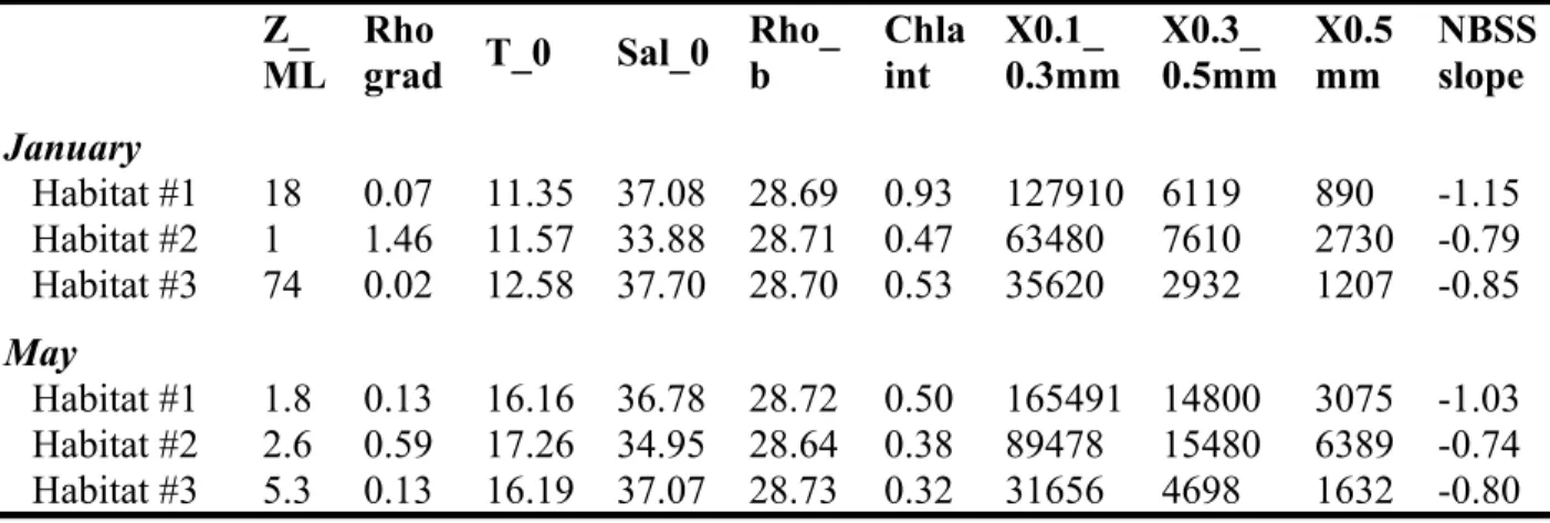
139 Based on the same cruises, three habitats were defined, characterized by physical parameters such
140 as sea surface salinity, sea surface temperature, bottom potential density, mixed layer depth and
141 stratification index, and biological conditions such as chl-a concentration, particle abundances for
142 3 size classes and the slope of the normalized biomass size spectrum (NBSS) (Table S1, E2014).
143 Habitat #1 was in the near shore area with shallow waters, steep NBSS slope and high chl-a
144 concentration; habitat #2 was representative of the zone of dilution of the Rhône plume with
145 stratified waters and flat NBSS slope; and habitat #3 was on the continental shelf with deep mixed
146 layer depth, lowest particle concentrations and intermediate NBSS slope.
147
148 2.2. LOPC data processing
149 Counts and sizes of particles sampled were extracted from the LOPC downcast profiles between 2
150 m depth below the sea surface and 5 m above the sea bottom. Abundance estimates by the LOPC
151 are dependent on the correct estimation of sampled volume (hereinafter SV). SV can either be
152 estimated from flow speed calculated using the manufacturers equation or estimated based on the
153 depth increment acquired together with LOPC counts. Using the manufacturers equation requires
283 284 285 286 287 288 289 290 291 292 293 294 295 296 297 298 299 300 301 302 303 304 305 306 307 308 309 310 311 312 313 314 315 316 317 318 319 320 321 322 323 324 325 326 327 328 329 330 331 332 333 334
7
154 that enough particles flow through the sampling tunnel. We used the manufactures equation when
155 the number of particles between 150 and 300 μm was > 30 per sample, otherwise SV was estimated
156 as the product of the LOPC opening area by the depth increment. To avoid duplicate counts of
157 particles that can happen in strong wave conditions, LOPC data for which the depth increment was
158 less than 10 cm were removed (5.1 % of the data). All data were processed using an in-house
159 program developed using matlab software (Mathworks, USA). At very high particle densities (>106
160 counts m-3), the data acquisition frequency of the LOPC might not be sufficient. This results first
161 in incoherent M sequences (data stream containing MEP characteristics), and second in the creation
162 of false MEPs due to the coincidence effect of counting at the same time several neighboring
163 particles as one large particle (Schultes and Lopes, 2009; Ohman et al., 2012; Basedow et al., 2014).
164 Incoherent M sequences were observed at 9 out of 135 stations, all of which showed a strong
165 density gradient. If the ratio of MEPs to total LOPC counts (TC) is above 5 % this might indicate
166 coincidence counts (Schultes and Lopes, 2009). We observed ratios above 5 % at 5 out of 135
167 stations, all located near shore.
168
169 2.3. Net sample processing using ZooScan
170 An aliquot from each net tow sample was processed using the ZooScan (www.zooscan.com) to
171 calculate the vertically integrated abundances and size structure of the zooplankton communities.
172 The net tow sample was split using a Motoda box ensuring a minimum of 1000 particles to be
173 identified by the Zooscan. Each scanned image had a resolution of 2400 dots per inch and was
174 analyzed using ZooProcess (Gorsky et al., 2010), which is embedded in ImageJ, an image analysis
175 software (Rasband, 2005). A total of 46 variables, including geometrical and optical characteristics,
176 are measured by Zooprocess for each individual larger than 300 μm ESD, and are used by the
177 Plankton Identifier software (Gasparini, 2007) to automatically classify the organisms following
339 340 341 342 343 344 345 346 347 348 349 350 351 352 353 354 355 356 357 358 359 360 361 362 363 364 365 366 367 368 369 370 371 372 373 374 375 376 377 378 379 380 381 382 383 384 385 386 387 388 389 390 391
8
178 the supervised learning algorithms implemented in the TANAGRA free statistical pack
179 (Rakotomalala, 2005). The Random forest algorithm was used for the classification analysis
180 (Breiman, 2001). Two predefined groups were created for the purpose of this study: organisms and
181 detritus. The ‘organisms’ group was mainly constituted of copepods (Carlotti, Unpublished data);
182 and the ‘detritus’ group was a composite category composed of phytoplankton aggregates and
183 undetermined fragments of organisms, such as gelatinous parts, molts etc. Most of these detrital
184 particles are created during the net tow by the pressure of the water against the mesh net and by the
185 aggregation of the material inside the cod-end. Therefore, this detritus cannot be related to those
186 counted in situ by the LOPC and was discarded from the ZooScan counts. After the automatic
187 sorting, all images were validated manually.
188
189 2.4. Calculation of normalized biomass size spectra
190 Normalized biomass size spectra (NBSS) were computed from LOPC and ZooScan data. For the
191 ZooScan, the ESD was calculated from the image area of a particle provided by ZooProcess.
192 For both data, the biovolume was derived from the ESD using the formula:
193
𝐵𝑖𝑜𝑉 = 𝐸𝑆𝐷
3×
𝜋 (1)6 × 𝑅
194 R, taken equal to 3, is the ratio of the major axis to minor axis of a prolate spheroid and we used 195 an organism density of 1 mg WW mm-3 to convert the biovolume into biomass. The NBSS were
196 calculated for each station using the method described in Herman and Harvey (2006). The linear
197 regressions were fitted to the part of a spectrum in the size range starting from the mode of the
198 spectrum in the small size and ending at the first empty size class.
199
200 2.5. LOPC derived indicators
395 396 397 398 399 400 401 402 403 404 405 406 407 408 409 410 411 412 413 414 415 416 417 418 419 420 421 422 423 424 425 426 427 428 429 430 431 432 433 434 435 436 437 438 439 440 441 442 443 444 445 446
9
201 We investigated two potential indicators that might reflect the proportion of detritus in LOPC
202 counts: (1) the proportion of MEPs in the total number of counts (%MEPs) and (2) the AI indicating
203 the transparency of particles. The theoretical size threshold between SEP and MEP is about 1.5
204 mm (Herman et al., 2004), but MEPs generally have a small ESD relatively to their maximum
205 length because they do not attenuate much light. We hypothesize that, in a region where most of
206 the organisms are below 1.5 mm of ESD (about 2.5 mm length for a copepod), the MEPs are mainly
207 composed of detritus so that the %MEPs mainly varies as a function of detritus concentration.
208 The attenuance index (AI) was calculated based on Checkley et al. (2008) and updated by Basedow
209 et al. (2013),
210
𝐴𝐼 = ∑
𝑛 ‒ 1𝑖 = 2𝐷𝑆
𝑖((𝑛 ‒ 1) ‒ 1) × 𝑚𝑎𝑥𝐷𝑆1 (2)211 where DS is the digital size of the MEP for each photodiode element, n the number of elements
212 and maxDS is the maximum digital size of a MEP (corresponding to a complete occlusion of a
213 diode element). Based on the definition, AI varies from 0 for very transparent particles to 1 for
214 very opaque particles. The DS values of the elements at the edges of the MEP sequence were not
215 included to compute the AI, because these elements may only partly cover the area of a diode,
216 resulting in a lower AI than real (Basedow et al., 2013). The AI should not be understood as an
217 opacity index only, because both opacity and shape of a particle contribute to it. For example, a
218 filamentous diatom (opaque but with lots of empty space) and an appendicularian (a very
219 transparent organism) could have a similar ESD and AI because they would attenuate the same
220 quantity of light, but they could have very different biovolume and opacity characteristics.
221
222 2.6. Estimation of the detritus part in LOPC counts
451 452 453 454 455 456 457 458 459 460 461 462 463 464 465 466 467 468 469 470 471 472 473 474 475 476 477 478 479 480 481 482 483 484 485 486 487 488 489 490 491 492 493 494 495 496 497 498 499 500 501 502 503
10
223 In the ocean, particulate matter consists of various types of particles including detrital aggregates,
224 decaying fragments of organisms, fecal pellets and sediments (Alldredge and Silver, 1988), which
225 will be called detritus hereafter. A total of 78 quasi-synchronous LOPC casts and net tows was
226 analyzed. Because the reliability and accuracy of abundance assessment with the ZooScan is very
227 high, the estimated abundance in the group ‘organisms’ was used as reference for zooplankton
228 abundance in this study. Nevertheless, it is important to keep in mind that nets are biased estimators
229 of the in-situ abundance of organisms that undersample fragile organisms and are limited to a
230 certain size range. Also, net avoidance by mobile organism and net clogging can bias abundance
231 estimates, but were unlikely to be an issue in our study. The size of copepods in the Mediterranean
232 Sea is generally small and the largest individuals of the dominant taxa Paracalanus and
233 Clausocalanus are about 1 mm length at the adult stage (Gaudy et al., 2003) limiting their escaping 234 capability. Moderate chl-a concentrations (maximum of 2.75 mg m-3) measured during the cruises
235 prevented the net from clogging (mesh size 120 μm).
236 The size range of zooplankton captured quantitatively is limited by the mesh size for the net
237 samples and the volume filtered for the LOPC (Vandromme et al., 2012). Based on the NBSS, we
238 estimated that the valid overlap in size range with correct estimation of abundance from both the
239 ZooScan and LOPC was from 350 μm to 2000 µm ESD.
240 We hypothesize as Vandromme et al. (2014) that within this size range the difference between the
241 ZooScan and LOPC is due to particulate matter counted in addition to zooplankton by the LOPC.
242 For size fraction i=350 to 2000 µm, the percentage of detritus in LOPC abundances was calculated
243 following the equation:
244 % detritusi = (LOPC_abi - ZooScan_abi) / LOPC_abi (3)
245 ZooScan abundances were higher than LOPC abundances at 14 stations out of 78, albeit only
246 slightly for 11 of them (< 30%), the stations being distributed over the gulf without any detectable
507 508 509 510 511 512 513 514 515 516 517 518 519 520 521 522 523 524 525 526 527 528 529 530 531 532 533 534 535 536 537 538 539 540 541 542 543 544 545 546 547 548 549 550 551 552 553 554 555 556 557 558
11
247 pattern. These stations were not included in the statistical analysis. The factors potentially leading
248 to this situation and the implications for this study are discussed later.
249 250
251 2.7. Statistical analyses
252 The Kruskal-Wallis test (one way ANOVA on ranks) was performed to identify potential links
253 between the percentage of detritus and LOPC particle characteristics (AI and %MEPs) on one hand,
254 and between percentage of detritus and the zooplankton habitats representative of different
255 environmental conditions on the other hand. This test was chosen because of the non-normal
256 distribution of the variables. Post-hoc tests were performed to assess the differences between
257 habitats. All statistical tests were performed using the R statistical software (version 3.2.3, R
258 Development Core Team, 2016), Kruskal-Wallis using kruskal.test and and post-hoc tests,
259 posthoc.kruskal.nemenyi.test (package PCMCR, version 2016-01-06).
260 261 262 263 264 265 266 267 268 269 270 563 564 565 566 567 568 569 570 571 572 573 574 575 576 577 578 579 580 581 582 583 584 585 586 587 588 589 590 591 592 593 594 595 596 597 598 599 600 601 602 603 604 605 606 607 608 609 610 611 612 613 614 615
12 271
272 273
274 3. Results
275 3.1. Spatiotemporal distribution of particle characteristics and detritus
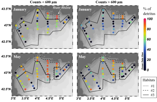
276 Fig. 1. Percentage of detritus in LOPC counts in January 2011 (top) and May 2010 (bottom) in the
277 Gulf of Lion for two particle size fractions: below (left) and above (right) 600 μm size. The three
278 habitats defined in Espinasse et al. 2014 are delineated, habitat #1: near shore area; habitat #2: area
279 affected by the Rhône waters; habitat #3: continental shelf.
280
281 The variability of the detritus in terms of spatial and temporal distribution was analyzed for two
282 size fractions, above and below 600 μm ESD (corresponding roughly to a total length of 1 mm for
283 a copepod) (Fig. 1). For both seasons, the percentage of detritus in LOPC counts was lower for the
284 larger size fraction than for the smaller one while their spatial patterns were similar. In winter, the
285 percentage of detritus of both small and large size was relatively low (mainly under 50%), except
619 620 621 622 623 624 625 626 627 628 629 630 631 632 633 634 635 636 637 638 639 640 641 642 643 644 645 646 647 648 649 650 651 652 653 654 655 656 657 658 659 660 661 662 663 664 665 666 667 668 669 670
13
286 for the three stations closest to the Rhône mouth. In spring, detritus represented a large part of the
287 LOPC counts (mainly over 50%) in the entire continental shelf. Only at the easternmost transect,
288 influenced by offshore water, a lower percentage of detritus was observed.
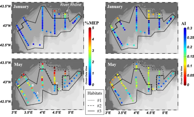
289 Fig. 2. Indicators of particles counted by the LOPC in January 2011 (top) and May 2010 (bottom)
290 in the Gulf of Lion: % of MEPs in total LOPC counts (left side) and the MEPs’ mean attenuance
291 index (AI, right side). The three habitats defined in Espinasse et al. 2014 are delineated, habitat #1:
292 near shore area; habitat #2: area affected by the Rhône waters; habitat #3: continental shelf. The
293 three representative stations (A, B and C) shown in Fig. 4 are marked in the lower left panel.
294
295 Throughout the study area, spatiotemporal differences in LOPC particle counts and characteristics
296 were observed (Fig. 2). In spring, higher values (> 2%) of the percentage of MEPs in total LOPC
297 counts were generally observed compared to winter (< 1%). However, high values were observed
298 in front of the Rhône mouth in winter and low values beyond the continental slope in spring. The
299 AI of the MEPs showed a pattern rather similar to the %MEPs (Fig.2, right panels). Some
300 differences existed, such as low values for the near shore area in the western part of the gulf in
675 676 677 678 679 680 681 682 683 684 685 686 687 688 689 690 691 692 693 694 695 696 697 698 699 700 701 702 703 704 705 706 707 708 709 710 711 712 713 714 715 716 717 718 719 720 721 722 723 724 725 726 727
14
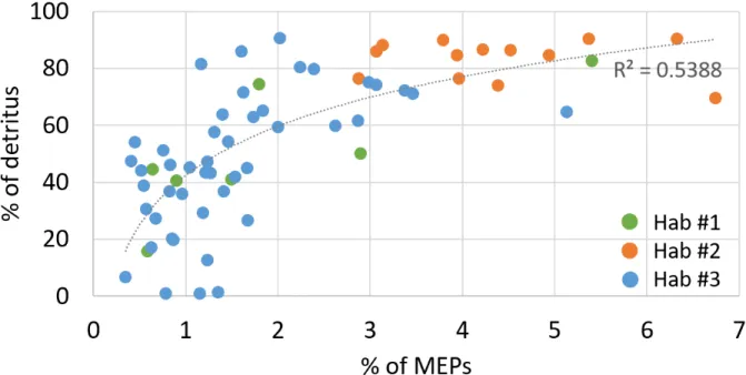
301 winter and high values for some stations in the most western transect in spring. A highly significant
302 correlation was found between the percentage of detritus and the %MEPs (r2=0.54, p <10-9)
303 strongly supporting our hypothesis that the %MEPs can be used as an indicator of detritus (Fig. 3).
304
305
306 Fig. 3. Percentage of detritus in LOPC counts relative to the percentage of MEPs in total LOPC
307 counts. The data were fitted with a logarithmic function. Habitats as defined in Fig. 1 and 2.
308
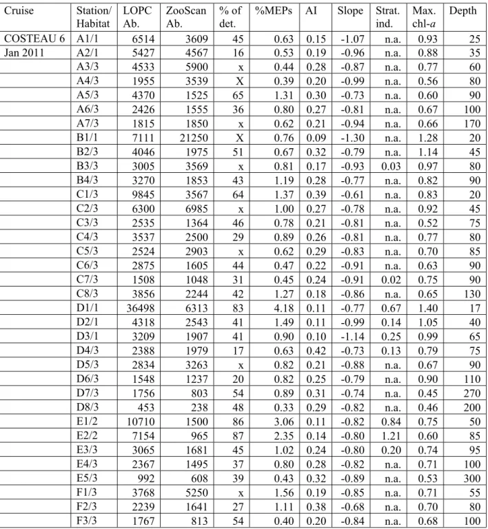
309 3.2. Statistical relationships between environmental conditions and LOPC indicators 310 Station details including LOPC and ZooScan abundances (# part. m-3), percentage of detritus in LOPC
311 counts, percentage of MEPs in LOPC counts, mean AI, slope of the NBSS, water column stratification 312 index, maximum of chl-a concentration (mg m-3) and sampling depth. Considering the station denotation,
313 the letter specifies the transect, from west (A) to east (F), and the number the position of the station along 314 the transect from coast (1) to offshore (6-8). For example, A1 is the furthest west station and E1 is located 315 in front of the mouth of the River Rhône. The stations A, B and C displayed in Figs 4-5 are indicated. No 316 stratification is stated as n.a. for non-applicable. When ZooScan counts were higher than LOPC counts 317 and, therefore, the percentage of detritus cannot be computed, x states for < 30 % difference in count and 318 X > 30%. Cruise Station/ Habitat LOPC Ab. ZooScan Ab. % of det.
%MEPs AI Slope Strat. ind. Max. chl-a Depth 731 732 733 734 735 736 737 738 739 740 741 742 743 744 745 746 747 748 749 750 751 752 753 754 755 756 757 758 759 760 761 762 763 764 765 766 767 768 769 770 771 772 773 774 775 776 777 778 779 780 781 782
15
COSTEAU 6 A1/1 6514 3609 45 0.63 0.15 -1.07 n.a. 0.93 25
Jan 2011 A2/1 5427 4567 16 0.53 0.19 -0.96 n.a. 0.88 35
A3/3 4533 5900 x 0.44 0.28 -0.87 n.a. 0.77 60 A4/3 1955 3539 X 0.39 0.20 -0.99 n.a. 0.56 80 A5/3 4370 1525 65 1.31 0.30 -0.73 n.a. 0.60 90 A6/3 2426 1555 36 0.80 0.27 -0.81 n.a. 0.67 100 A7/3 1815 1850 x 0.62 0.21 -0.94 n.a. 0.66 170 B1/1 7111 21250 X 0.76 0.09 -1.30 n.a. 1.28 20 B2/3 4046 1975 51 0.67 0.32 -0.79 n.a. 1.14 45 B3/3 3005 3569 x 0.81 0.17 -0.93 0.03 0.97 80 B4/3 3270 1853 43 1.19 0.28 -0.77 n.a. 0.82 90 C1/3 9845 3567 64 1.37 0.39 -0.61 n.a. 0.83 20 C2/3 6300 6985 x 1.00 0.27 -0.78 n.a. 0.92 45 C3/3 2535 1364 46 0.78 0.21 -0.81 n.a. 0.52 75 C4/3 3537 2500 29 0.89 0.26 -0.81 n.a. 0.77 80 C5/3 2524 2903 x 0.62 0.29 -0.83 n.a. 0.70 85 C6/3 2875 1605 44 0.47 0.22 -0.91 n.a. 0.63 90 C7/3 1508 1048 31 0.45 0.24 -0.91 0.02 0.75 90 C8/3 3856 2244 42 1.27 0.18 -0.86 n.a. 0.65 130 D1/1 36498 6313 83 4.18 0.11 -0.77 0.67 1.40 17 D2/1 4318 2543 41 1.49 0.11 -0.99 0.14 1.05 40 D3/1 3209 1907 41 0.90 0.10 -1.14 0.25 0.99 65 D4/3 2388 1979 17 0.63 0.42 -0.73 0.13 0.79 75 D5/3 2834 3263 x 0.82 0.21 -0.88 n.a. 0.67 90 D6/3 1548 1237 20 0.82 0.25 -0.79 n.a. 0.90 110 D7/3 1756 803 54 0.89 0.31 -0.74 n.a. 0.45 270 D8/3 453 238 48 0.33 0.29 -0.82 n.a. 0.46 200 E1/2 10710 1500 86 3.06 0.11 -0.82 0.84 0.75 50 E2/2 7154 965 87 2.35 0.14 -0.80 1.21 0.60 85 E3/3 3065 1681 45 1.02 0.24 -0.80 0.20 0.74 95 E4/3 2367 1495 37 0.80 0.28 -0.82 n.a. 0.71 100 E5/3 992 608 39 0.43 0.32 -0.89 n.a. 0.53 300 F1/3 3768 5250 x 1.56 0.19 -0.85 n.a. 0.71 55 F2/3 2239 1641 27 1.11 0.38 -0.68 n.a. 0.70 80 F3/3 1767 813 54 0.40 0.20 -0.84 n.a. 0.68 100 F4/3 1257 1174 7 0.33 0.26 -0.95 n.a. 0.70 130 COSTEAU 4 A1/1 5924 9851 X 1.29 0.08 -1.02 0.06 1.70 25 May 2010 A2/1 15354 7646 50 2.90 0.09 -1.03 0.11 2.43 36 A3/3 5343 3021 43 1.22 0.17 -0.89 0.05 0.87 55 A4/3 4733 1361 71 3.46 0.23 -0.64 0.03 0.58 80 A5/3 4168 1599 62 2.82 0.25 -0.66 0.03 0.63 80 A6/3 3946 1462 63 1.73 0.22 -0.82 0.04 0.46 100 A7/3 3088 287 91 2.00 0.25 -0.71 0.03 0.50 145 B1/2 19440 5070 74 4.37 0.11 -0.79 0.29 0.33 20 B2/1 10675 2725 74 1.78 0.10 -0.99 0.18 1.68 50 B3/3 7298 1887 74 3.06 0.11 -0.87 0.20 0.73 80 Stn. B B4/3 3933 1597 59 2.00 0.14 -0.78 0.17 0.53 90 787 788 789 790 791 792 793 794 795 796 797 798 799 800 801 802 803 804 805 806 807 808 809 810 811 812 813 814 815 816 817 818 819 820 821 822 823 824 825 826 827 828 829 830 831 832 833 834 835 836 837 838 839
16 B5/3 2373 462 81 2.24 0.18 -0.74 0.11 0.82 150 Stn. A B6/3 1687 1736 x 1.15 0.24 -0.80 0.04 1.10 200 B7/3 2271 1433 37 1.41 0.16 -0.90 0.15 0.55 265 B8/3 1411 1392 1 1.35 0.15 -0.92 0.10 0.76 200 C1/2 44544 13513 70 4.44 0.22 -0.62 0.47 0.43 20 C2/2 10514 1622 85 2.07 0.13 -0.87 0.28 1.35 45 C3/3 5109 2046 60 1.89 0.14 -0.85 0.23 0.80 75 C5/3 8609 2382 72 3.24 0.22 -0.65 0.25 0.90 90 C6/3 8902 3134 65 4.50 0.15 -0.75 0.27 0.61 90 C7/3 5193 1294 75 2.43 0.16 -0.76 0.36 0.91 85 C8/3 3491 993 72 1.62 0.15 -0.85 0.24 0.41 140 D1/2 33804 3244 90 5.87 0.12 -0.68 0.61 0.77 15 D2/2 21171 3231 85 4.93 0.14 -0.62 0.41 0.69 40 D3/2 16739 2239 87 4.22 0.13 -0.72 0.54 0.90 65 D4/2 15823 1856 88 3.13 0.15 -0.71 0.74 1.20 75 D5/2 11200 2645 76 2.87 0.16 -0.66 1.05 1.13 95 Stn. C D6/2 8968 905 90 3.79 0.12 -0.68 0.51 2.27 115 D7/3 4356 613 86 1.58 0.16 -0.89 0.40 0.49 200 D8/3 1257 664 47 1.23 0.21 -0.79 0.25 0.59 200 E1/2 40713 3925 90 5.21 0.15 -0.60 2.10 2.73 50 E2/2 15312 3602 76 3.97 0.15 -0.72 0.71 2.70 90 E3/3 10570 2130 80 2.38 0.23 -0.74 0.31 0.44 95 E4/3 2734 1503 45 1.65 0.24 -0.74 0.07 0.54 100 E5/3 2047 869 58 1.31 0.27 -0.76 0.06 0.49 200 E6/3 2284 2922 x 1.29 0.20 -0.82 0.05 1.35 200 F1/3 4991 5357 x 1.96 0.19 -0.79 0.02 0.73 60 F2/3 2679 2340 13 1.22 0.22 -0.78 0.05 0.45 80 F3/3 4086 755 82 1.15 0.19 -0.83 0.07 0.40 100 F4/3 1816 1455 20 0.86 0.24 -0.83 0.03 0.54 200 F5/3 1799 1307 27 0.67 0.24 -0.90 0.01 0.76 200 F6/3 1645 2046 x 1.01 0.25 -0.83 0.02 0.55 200 319 320
321 To get a better understanding of the mechanisms underlying the relationship between the %MEPs
322 and the detritus abundances, we tracked how they changed with different environmental conditions
323 (Table 1) as described by the three habitats defined in E2014. The percentage of detritus, percentage
324 of MEPs and AI changed significantly between the habitats defined in E2014 (Table 2). The area
325 affected by the Rhône River freshwater (defined as habitat #2) had a significantly higher percentage
326 of detritus and a higher %MEPs than the other two habitats. The average %MEPs in habitat #2 was
327 2.48 (2.18-3.07, n = 3) in January and 3.51 (2.07-5.88, n = 17) in May compared to an overall
843 844 845 846 847 848 849 850 851 852 853 854 855 856 857 858 859 860 861 862 863 864 865 866 867 868 869 870 871 872 873 874 875 876 877 878 879 880 881 882 883 884 885 886 887 888 889 890 891 892 893 894
17
328 average of 1.65 (0.67-4.59, n = 48) and 0.67 (0.32-4.18, n = 67) for habitats #1 and #3. The
329 continental shelf (habitat #3) was characterized by particles with a significantly higher AI, overall
330 average of 0.23 (0.09-0.43, n = 97), than for habitats #1 and #2, overall average of 0.11 (0.07-0.19,
331 n = 18) and 0.14 (0.10 – 0.22, n = 20), respectively. The changes in distribution of detritus, %MEPs
332 and AI within the habitats showed that the conditions where stratified waters were coupled with
333 high chl-a concentrations in the surface layer resulted in a higher percentage of detritus and a higher
334 %MEPs. This was observed in habitat #2 influenced by Rhône waters. The lower AI and higher
335 percentage of detritus in habitat #2 demonstrated the general transparency of the detritus, compared
336 to the higher AI associated with lower detritus observed on the continental shelf (habitat #3).
337
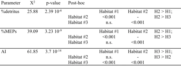
338 Table 2. Kruskal-Wallis test applied on the percentage of detritus, % of MEPs and AI considering
339 as factors the 3 habitats defined in Espinasse et al. 2014. Post-hoc results are also shown.
340 341 342 343 344 345
Parameter Χ2 p-value Post-hoc
%detritus 25.88 2.39 10-6 Habitat #1 Habitat #2 Habitat #2 <0.001 -Habitat #3 n.s. <0.001
H2 > H1; H2 > H3 %MEPs 39.09 3.23 10-9 Habitat #1 Habitat #2
Habitat #2 <0.001 -Habitat #3 n.s. <0.001 H2 > H1; H2 > H3 AI 61.85 3.7 10-14 Habitat #1 Habitat #2 Habitat #2 n.s. -Habitat #3 <0.001 <0.001 H3 > H1; H3 > H2 899 900 901 902 903 904 905 906 907 908 909 910 911 912 913 914 915 916 917 918 919 920 921 922 923 924 925 926 927 928 929 930 931 932 933 934 935 936 937 938 939 940 941 942 943 944 945 946 947 948 949 950 951
18 346
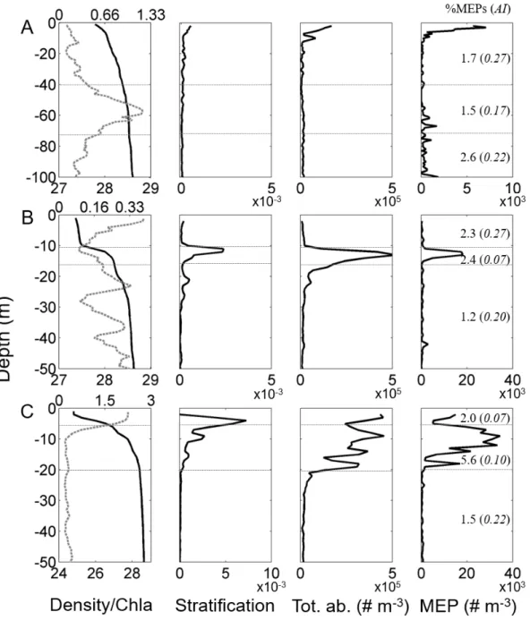
347 3.3. Detailed analyses of particle characteristics at three typical stations 348
349 Fig. 4. Vertical profiles of water density σθ (kg m-3; full line, left panels) and chl-a concentration 350 (mg m-3; dashed grey line, left panels), the stratification (Brunt-Väisälä frequency squared N2, s-2 ;
351 center left panels), total LOPC abundance (Tot. ab., centre right panels) and MEP abundance (right
352 panels) at stations A, B and C typical of different environmental conditions. The integrated % of
353 MEPs and the average of AI are specified in brackets for two (station A) or three (stations B and
955 956 957 958 959 960 961 962 963 964 965 966 967 968 969 970 971 972 973 974 975 976 977 978 979 980 981 982 983 984 985 986 987 988 989 990 991 992 993 994 995 996 997 998 999 1000 1001 1002 1003 1004 1005 1006
19
354 C) depth layers (horizontal dotted grey lines). The location of the stations is shown in Fig. 2. Note
355 the change in x-axis range among stations.
356 Based on the results provided by the spatial distributions, three stations representing different
357 scenarios in terms of water stratification and chl-a concentration were chosen to investigate the
358 vertical variations of TC, MEPs, %MEPs and AI (Fig. 4).
359 Vertical profiles at station A showed a homogeneous water density and Brunt-Väisälä frequency,
360 and a deep peak of chl-a concentration reaching 1.2 mg chl-a m-3 at 60 m depth. TC and MEP
361 counts had a peak in the surface layer, reached minima between 20 and 40 m, and slightly increased
362 in the layer between 40 and 70 m and the layer below, while AI was lower in the layer of maximum
363 of chl-a. At this station, %MEPs and average AI integrated over the entire water column were 1.15
364 and 0.24, respectively, and the percentage of detritus was estimated to be of 0% (i.e. LOPC
365 abundance = ZooScan abundance).
366 Profiles at station B showed a stratified water column with a pycnocline located at 12 m depth and
367 relatively low chl-a concentration (0.09-0.36 mg chl-a m-3). TC and MEP counts peaked in the
368 pycnocline layer. The AI was high in the surface layer (0.27) and dropped strongly in the
369 pycnocline layer to 0.07. %MEPs was relatively high in the surface layer and increased below the
370 pycnocline. At this station, %MEPs and average AI integrated over the entire water column were
371 2.00 and 0.14, respectively, and the percentage of detritus was estimated to be of 59% in LOPC
372 counts.
373 Station C was located in the Rhône plume, approximately at 45 km from the Rhône mouth, showing
374 a thin layer of very low salinity water in surface resulting in strong stratification. Highest chl-a
375 concentrations were found in the surface layer (maximum of 2.3 mg chl-a m-3). The halocline layer
376 between surface low salinity water and deep saltier water was spread between 5 and 20 m depth.
377 High LOPC abundance and very high MEP abundance were found in the surface and gradient
1011 1012 1013 1014 1015 1016 1017 1018 1019 1020 1021 1022 1023 1024 1025 1026 1027 1028 1029 1030 1031 1032 1033 1034 1035 1036 1037 1038 1039 1040 1041 1042 1043 1044 1045 1046 1047 1048 1049 1050 1051 1052 1053 1054 1055 1056 1057 1058 1059 1060 1061 1062 1063
20
378 layers. Very low AI values were observed in the surface layer, and low AI values and very high
379 values of %MEPs were found in the halocline. Below the stratified layer these parameters were
380 similar to those at stations A and B. At station C, %MEPs and average AI integrated over the entire
381 water column were 3.79 and 0.12, respectively, and the percentage of detritus was estimated to be
382 up to 90% in LOPC abundance (i.e. LOPC abundance was 10 times the zooplankton abundance
383 estimated with the ZooScan).
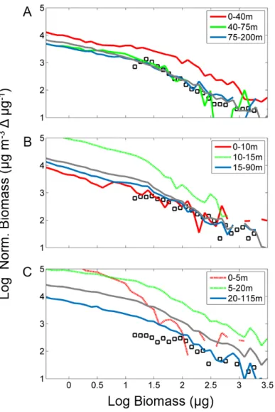
384 The NBSSs of particles estimated for the whole water column by both devices showed good
385 agreement in their size range overlap (1.1 to 3.4 log(µg)) for the stations A and B (Fig. 5), but
386 relatively high difference for the station C with higher biomasses from LOPC. NBSS inside the
387 different water layers provides information on the homogeneity of the biomass distribution as a
388 function of depth. The NBSSs at station A were vertically homogeneous, although the biomass in
389 the surface layer was slightly higher. The NBSSs at station B and C showed much higher values in
390 the stratified layers. At station C, the NBSS in the surface layer was characterized by high biomass
391 values in the lower size classes and a relatively steep NBSS slope (-1.21) towards higher size
392 classes, which is a signature of productive layer. In the halocline and below, the NBSS slopes were
393 flatter (-0.64 and -0.79) and similar in shape, potentially resulting from a uniform distribution of
394 the detritus along the size spectrum.
395 396 397 398 399 400 1067 1068 1069 1070 1071 1072 1073 1074 1075 1076 1077 1078 1079 1080 1081 1082 1083 1084 1085 1086 1087 1088 1089 1090 1091 1092 1093 1094 1095 1096 1097 1098 1099 1100 1101 1102 1103 1104 1105 1106 1107 1108 1109 1110 1111 1112 1113 1114 1115 1116 1117 1118
21
401 Fig. 5. Normalized biomass size spectra (NBSS) from LOPC data integrated over the water column
402 (grey line) and in different layers as defined in Fig. 4 (blue lines, NBSSs in stratified layers are
403 displayed with dashed line), and NBSS from ZooScan data over the whole water column (black
404 squares) for 3 stations typical of different environmental conditions (see Fig. 2 and 4).
405 406 407 408 409 1123 1124 1125 1126 1127 1128 1129 1130 1131 1132 1133 1134 1135 1136 1137 1138 1139 1140 1141 1142 1143 1144 1145 1146 1147 1148 1149 1150 1151 1152 1153 1154 1155 1156 1157 1158 1159 1160 1161 1162 1163 1164 1165 1166 1167 1168 1169 1170 1171 1172 1173 1174 1175
22
410 3.4. Typical distribution of particles and LOPC indicators under specific environmental
411 conditions
412 Four typical associations between particle distribution and environment could be identified from
413 the detailed analyses of the stations:
414 (1) Vertical density stratification coincided with a peak in LOPC counts. To test this statement, we
415 investigated the occurrences of a peak of LOPC abundance in relation to the occurrences of a
416 strongly stratified layer at all stations. A peak of LOPC counts was defined for concentrations > 50
417 % of the average concentration over the whole profile. Stratified layers were defined using a
418 threshold value of N2 = 0.001 s-2 (Brunt-Väisälä frequency). A co-occurrence between a
419 stratification layer and a peak of LOPC counts was found for 93 % of the stations (81 out of 87
420 stratified stations, χ2 test, p< 10-9).
421 (2) The percentage of MEPs in total LOPC counts increased when stratification was associated
422 with high chl-a concentrations (chl-a > 1 mg m-3) in the surface layer. Density gradients in the
423 water column typically lead to aggregate formation, and the number of aggregates increase with
424 high production in the surface layer resulting in more MEPs, which is illustrated in the MEP profile
425 and NBSS comparison at station C (Fig. 4 and 5). It was also indirectly confirmed by the changes
426 in AI values as a function of size: larger MEPs (> 1.5 mm) were very transparent (mean 0.21, std
427 0.10) in the stratified layer compared to the other layers (mean 0.50, std 0.18; Fig. 6b).
428 (3) Situations without stratification and with high chl-a concentrations were associated with a low
429 AI and a relatively low %MEPs (Figs 2 and 4). This situation is exemplified in the surface layer at
430 station C, and to a lesser extent in the middle layer (40 to 75 m depth) at station A. It also
431 corresponds roughly to all the stations within habitat #1, characterized by mixed waters and high
432 chl-a concentrations (Fig. 2). In such situations, the peak in MEP size spectra appears to be shifted
433 towards smaller size classes (Fig. 6a). Accordingly, MEP size in habitat #1 was generally much
1179 1180 1181 1182 1183 1184 1185 1186 1187 1188 1189 1190 1191 1192 1193 1194 1195 1196 1197 1198 1199 1200 1201 1202 1203 1204 1205 1206 1207 1208 1209 1210 1211 1212 1213 1214 1215 1216 1217 1218 1219 1220 1221 1222 1223 1224 1225 1226 1227 1228 1229 1230
23
434 smaller than in habitat #2 (high chl-a concentration and stratification), with an average of 505 μm
435 ESD (406-705 μm) and 823 μm ESD (619-1387 μm), respectively.
436 (4) The AI stayed relatively constant over all the stations without stratification or high chl-a
437 concentration with an average value of 0.25 (std 0.05).
438
439 Fig. 6. (a) Size spectra of MEPs and (b) mean attenuance index (AI) as a function of the MEP size
440 (0.1 mm interval) at station C (see Fig. 2, 4 & 5) in 3 different water layers. Because of lower
441 values, MEP abundances for the deepest layer (20-115 m) is displayed on a separate axis (right).
442 443 444 1235 1236 1237 1238 1239 1240 1241 1242 1243 1244 1245 1246 1247 1248 1249 1250 1251 1252 1253 1254 1255 1256 1257 1258 1259 1260 1261 1262 1263 1264 1265 1266 1267 1268 1269 1270 1271 1272 1273 1274 1275 1276 1277 1278 1279 1280 1281 1282 1283 1284 1285 1286 1287
24 445 4. Discussion
446 4.1. Optimal conditions to use the LOPC as a zooplankton counter
447 Based on our dataset from the coastal waters of the Northwestern Mediterranean Sea, we identified
448 three main ecological situations where the LOPC counted various amounts of detritus. In
449 unstratified water columns with low chl-a concentrations (< 1 mg m-3), LOPC abundances were
450 comparable to net abundances, meaning that the LOPC counted mostly zooplankton and only few
451 detritus. This was reflected by LOPC particles having a low %MEPs in total counts (< 2 %), and a
452 high mean AI (> 0.2). In stratified waters with high chl-a concentrations, LOPC abundances were
453 up to ten times higher than net abundances most likely due to the LOPC counting detritus. In this
454 situation, LOPC counts were characterized by high %MEPs and low AIs. In stratified waters with
455 low chl-a concentrations, LOPC abundances were also higher than net abundances but in a lesser
456 extent, and particles here were again characterized by a high %MEPs and a low AI. These results
457 suggest that information on the large particles counted by the LOPC (MEPs) can be used to infer
458 the percentage of detritus counted by the LOPC. Our results also suggest that the LOPC counted
459 mainly living organisms when the %MEPs was < 2 %, a more conservative limit than the 5 % limit
460 found by Schultes and Lopes (2009) off the Brazilian coast. In most water columns without
461 stratification and/or high chl-a concentration the mean AI remained constant, around 0.25, which
462 allowed us to define a threshold below which aggregation or phytoplankton chains likely occur.
463 The usage of %MEPs and AI as indicators of different physical and biological situations is
464 summarized in Table 3. By applying our thresholds to the data from our study area and to data from
465 high latitudes, we could identify in total four different situations in which detritus represent
466 between 0 and 90 % of the total LOPC counts.
467 468 1291 1292 1293 1294 1295 1296 1297 1298 1299 1300 1301 1302 1303 1304 1305 1306 1307 1308 1309 1310 1311 1312 1313 1314 1315 1316 1317 1318 1319 1320 1321 1322 1323 1324 1325 1326 1327 1328 1329 1330 1331 1332 1333 1334 1335 1336 1337 1338 1339 1340 1341 1342
25 469
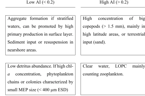
470 Table 3. Summary describing how to interpret the LOPC abundance with the help of the two
471 indicators, %MEPs and AI. The thresholds defined in this study lead to 4 situations. The possible
472 causes for these situations are detailed and clues to interpret the data based on the study context are
473 proposed. The threshold for overestimation (5 %) is from Schultes and Lopes 2009.
474
Low AI (< 0.2) High AI (> 0.2) High % of MEPs (> 2)
(> 5 overestimation)
Aggregate formation if stratified waters, can be promoted by high primary production in surface layer. Sediment input or resuspension in nearshore areas.
High concentration of big copepods (> 1.5 mm), mainly in high latitude areas, or terrestrial input (sand).
Low % of MEPs (< 2) Low detritus abundance. If high
chl-a concentrchl-ation, phytoplchl-ankton
chains or colonies characterized by small MEP size (< 400 µm ESD)
Clear water, LOPC mainly counting zooplankton.
475 476
477 4.2. Potential biases linked to the sampling protocol
478 The LOPC was placed on the CTD rosette to obtain simultaneous profiles of physical and
479 biogeochemical parameters and net tows were conducted afterwards. The time lag between a LOPC
480 cast and corresponding net tow could have affected the comparison between ZooScan and LOPC
481 results, even though it was reduced to its minimum. The general patchiness of particles and
482 zooplankton in the water column can create some variability in abundance data collected at the
483 same location over a short amount of time. In general however, the vertical distributions of particles
1347 1348 1349 1350 1351 1352 1353 1354 1355 1356 1357 1358 1359 1360 1361 1362 1363 1364 1365 1366 1367 1368 1369 1370 1371 1372 1373 1374 1375 1376 1377 1378 1379 1380 1381 1382 1383 1384 1385 1386 1387 1388 1389 1390 1391 1392 1393 1394 1395 1396 1397 1398 1399
26
484 measured by the LOPC along the coastal-offshore transects (stations separated by 5 km) showed
485 consistent abundances between the stations with gradual changes, suggesting a limited patchiness.
486 Furthermore, for the majority of the offshore stations with no stratification and low chl-a
487 concentration, the percentage of detritus was intermediate and rather constant (mean 39, standard
488 deviation 17). Therefore, we argue that even if patchiness potentially created some variability
489 blurring our results, especially where percentage of detritus was low, at most of our stations it was
490 valid to use a comparison of abundances to determine the detritus contribution. At 3 out of 78
491 stations, abundances determined from net samples were >30 % higher than those determined by
492 the LOPC, two of these stations being in shallow waters. We suggest that these values might be
493 due to technical issues (difference in sampling depth, mistake through the subsampling preparation,
494 etc.) and they were, therefore, not included in any part of the analysis.
495
496 4.3. Impact of stratification and/or high production on LOPC counts and the formation
497 of MEPs
498 The relationship between the detritus distribution and the habitats defined in E2014 (Table 2)
499 provided a good base to analyze the link between detritus formation and environmental conditions.
500 Consistent results were found analyzing the spatial distributions and the vertical profiles in the
501 changes of percentage of detritus, LOPC counts and MEP characteristics. The stratification of the
502 water column seems to be the main factor influencing the vertical distribution of LOPC counts.
503 The interface between water layers of different densities acts as a barrier, locally accumulating
504 particles. The high concentrations of particles within pycnoclines can be explained by the change
505 in buoyancy of aggregates, reducing their downward settling velocities (Macintyre et al., 1995,
506 Prairie et al., 2015). Our case study from the Mediterranean Sea shows that this process induces
507 particle aggregations resulting in the formation of transparent MEPs with a low AI (< 0.2), and in
1403 1404 1405 1406 1407 1408 1409 1410 1411 1412 1413 1414 1415 1416 1417 1418 1419 1420 1421 1422 1423 1424 1425 1426 1427 1428 1429 1430 1431 1432 1433 1434 1435 1436 1437 1438 1439 1440 1441 1442 1443 1444 1445 1446 1447 1448 1449 1450 1451 1452 1453 1454
27
508 an increase of the %MEPs in total counts (see again Fig. 1, situation described in the upper left part
509 of the Table 3). The mechanisms underlying the aggregate formation can be mechanical, due to
510 transparent exopolymer particles, mucus or dead phytoplankton cells (Alldredge and Silver, 1988),
511 or chemical, when strong salinity changes promotes flocculation processes. When such a
512 stratification is combined with high production in the surface layer, the higher concentration of
513 particles will promote the formation of more aggregates, resulting in very high %MEPs.
514 When high chl-a concentrations were not associated with stratification, the size of the MEPs was
515 smaller and the AI decreased below 0.2 while the %MEPs remained constant. One explanation is
516 that without stratification, settling particles could freely fall through the water column, and the
517 probability of colliding between particles is reduced. But also, phytoplankton colonies typically
518 produce small MEPs with lower AI due to a high degree of empty space at the activated
519 photodiodes. Further investigations at stations that show a large contribution of detritus could also
520 give insight into the changes of the size structure of organic matter in different water layers, which
521 could be useful to study carbon vertical flux.
522
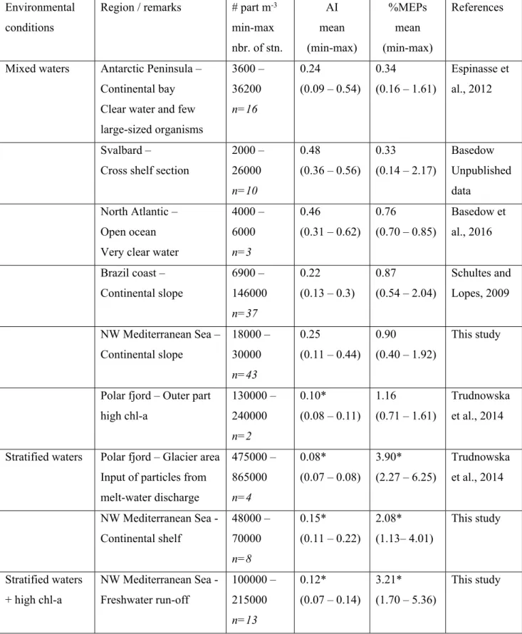
523 4.4. Limits of the methods
524 Our method is based on the information from the MEPs, which represent only a small part of the
525 LOPC counts, but we successfully extrapolated this result to assess the contribution of detritus in
526 the total LOPC counts. We suggest that there is a relationship between the % of SEPs being detritus
527 and the %MEPs in LOPC counts. Indeed, the aggregation processes described earlier in the text
528 (see 4.3) attest that if detritus represents a substantial part of the SEPs, some will aggregate and
529 end up as MEPs. This is due to the detritus constitution and has been described by several studies
530 focusing, for instance, on phytoplankton blooms (Alldredge and Jackson, 1995) or appendicularian
531 houses (Lombard and Kiørboe, 2010).
1459 1460 1461 1462 1463 1464 1465 1466 1467 1468 1469 1470 1471 1472 1473 1474 1475 1476 1477 1478 1479 1480 1481 1482 1483 1484 1485 1486 1487 1488 1489 1490 1491 1492 1493 1494 1495 1496 1497 1498 1499 1500 1501 1502 1503 1504 1505 1506 1507 1508 1509 1510 1511
28
532 In some specific cases the %MEPs can be affected by others causes than the ones described in this
533 study. In places with very clear water and high concentrations of big organisms, e.g. Calanus
534 finmarchicus overwintering in North Atlantic waters, the %MEPs can drastically rise even though 535 the percentage of detritus is low (Table 3, upper right). In that case, we suggest to use the AI alone
536 as an indicator to separate between living and non-living particles (Checkley et al., 2008; Gaardsted
537 et al., 2010), and estimate the part of the MEPs being detrtital particles. In this study, where the
538 dominating species were small copepods, we assume that MEPs that have a low AI were detritus.
539 However, transparent gelatinous organisms can also a have similar MEP signal. Given the opening
540 of the LOPC tunnel (7 x 7 cm), appendicularians are among potential organisms that can be counted
541 by the LOPC in amounts high enough to affect the MEP signal. In our case, although substantial
542 abundance of appendicularians were recorded during the winter cruise (ca 30 000 # m-2), this did
543 not seem to affect the MEP signal as the AI was higher in winter than during the spring cruise.
544 Nevertheless, we suggest that when using the LOPC, occasional net samples are needed to describe
545 the plankton community and to attest of peaks of specific groups such as gelatinous zooplankton.
546
547 4.5. Use of our results in other regions
548 The indicators developed in this study to interpret the detritus part of LOPC abundances are based
549 on a large dataset collected in a coastal area of the NW Mediterranean Sea. However, the processes
550 leading to the formation of detritus are not specific to this area. They take place in the epipelagic
551 zone of most of the marine ecosystems, and it is likely that these indicators will be valid in other
552 areas. To test this, we applied the thresholds for %MEPs and AI that were developed in this study
553 to other datasets from around the globe.
554 A dataset collected in a tropical system (Schultes and Lopes, 2009), sampled from mixed and
555 weakly stratified stations over the continental shelf and slope, had generally a low %MEPs (mean
1515 1516 1517 1518 1519 1520 1521 1522 1523 1524 1525 1526 1527 1528 1529 1530 1531 1532 1533 1534 1535 1536 1537 1538 1539 1540 1541 1542 1543 1544 1545 1546 1547 1548 1549 1550 1551 1552 1553 1554 1555 1556 1557 1558 1559 1560 1561 1562 1563 1564 1565 1566
29
556 0.87, standard deviation 0.33) and rather high AIs (mean 0.22, standard deviation 0.04) over 37
557 stations (Table 4). The biomass estimated with the LOPC for particles > 500 µm ESD was
558 significantly correlated to zooplankton displacement volume of net samples (n= 37, r= 0.4, p<
559 0.01), indicating a limited influence of detritus (Table 3, lower right).
560 Two datasets from polar areas (Antarctic Peninsula and Svalbard) were characterized by clear
561 water, and LOPC counts had a very low %MEPs (< 0.5 %) and generally high AIs (> 0.2). Here,
562 the indicators show that the LOPC counted mainly zooplankton (Table 3, lower right), which was
563 supported by a good agreement between LOPC and net data.
564 In an Arctic fjord characterized by glacial melt water input, freshwater run-off resulted in a
565 dramatic increase in LOPC counts (> 500 x 103 # m-3) in the inner part of the fjord and very low
566 AI values in the entire fjord (Trudnowska et al., 2014). The %MEPs, on the other hand, was
567 gradually decreasing from 3.90 in the inner part to 1.16 in the outer part while the zooplankton
568 abundances estimated from net tows were rather constant along the transect. Based on the
569 thresholds developed for the indicators %MEPs and AI, the fjord can be divided into two areas, i.e.
570 the inner part characterized by high %MEPs, low AIs and high (glacial) detritus concentrations
571 (Table 3, upper right); and the outer part characterized by low %MEPs, low AIs, high chl-a
572 concentration and realistic zooplankton abundances estimated by the LOPC (Table 3, lower left).
573 574 575 576 577 578 579 1571 1572 1573 1574 1575 1576 1577 1578 1579 1580 1581 1582 1583 1584 1585 1586 1587 1588 1589 1590 1591 1592 1593 1594 1595 1596 1597 1598 1599 1600 1601 1602 1603 1604 1605 1606 1607 1608 1609 1610 1611 1612 1613 1614 1615 1616 1617 1618 1619 1620 1621 1622 1623
30
580 Table 3. Comparison of particle characteristics in different regions and different environmental
581 conditions. Only stations deeper than 50 m were included. High chl-a: max chl-a > 1 mg m-3.
582 *data which are out of the optimal conditions for LOPC use (based on the thresholds defined in Table 2) Environmental
conditions
Region / remarks # part m-3
min-max nbr. of stn. AI mean (min-max) %MEPs mean (min-max) References
Mixed waters Antarctic Peninsula – Continental bay Clear water and few large-sized organisms 3600 – 36200 n=16 0.24 (0.09 – 0.54) 0.34 (0.16 – 1.61) Espinasse et al., 2012 Svalbard – Cross shelf section
2000 – 26000 n=10 0.48 (0.36 – 0.56) 0.33 (0.14 – 2.17) Basedow, Unpublished data North Atlantic – Open ocean Very clear water
4000 – 6000 n=3 0.46 (0.31 – 0.62) 0.76 (0.70 – 0.85) Basedow et al., 2016 Brazil coast – Continental slope 6900 – 146000 n=37 0.22 (0.13 – 0.3) 0.87 (0.54 – 2.04) Schultes and Lopes, 2009 NW Mediterranean Sea – Continental slope 18000 – 30000 n=43 0.25 (0.11 – 0.44) 0.90 (0.40 – 1.92) This study
Polar fjord – Outer part high chl-a 130000 – 240000 n=2 0.10* (0.08 – 0.11) 1.16 (0.71 – 1.61) Trudnowska et al., 2014
Stratified waters Polar fjord – Glacier area Input of particles from melt-water discharge 475000 – 865000 n=4 0.08* (0.07 – 0.08) 3.90* (2.27 – 6.25) Trudnowska et al., 2014 NW Mediterranean Sea - Continental shelf 48000 – 70000 n=8 0.15* (0.11 – 0.22) 2.08* (1.13– 4.01) This study Stratified waters + high chl-a NW Mediterranean Sea - Freshwater run-off 100000 – 215000 n=13 0.12* (0.07 – 0.14) 3.21* (1.70 – 5.36) This study 1627 1628 1629 1630 1631 1632 1633 1634 1635 1636 1637 1638 1639 1640 1641 1642 1643 1644 1645 1646 1647 1648 1649 1650 1651 1652 1653 1654 1655 1656 1657 1658 1659 1660 1661 1662 1663 1664 1665 1666 1667 1668 1669 1670 1671 1672 1673 1674 1675 1676 1677 1678
31 583 5. Conclusion
584 We defined thresholds for two indicators based on LOPC data, which allowed to quickly check the
585 contribution of detritus to total LOPC counts. These indicators were developed based on an
586 extensive dataset from the Gulf of Lion and showed to be successful in different marine
587 biogeographical regions. Applying the indicators %MEPs and AI provides a good basis to assess
588 the detrital part in LOPC counts. When the thresholds for %MEPs and AI indicate that the LOPC
589 is not mainly counting zooplankton, data should be interpreted carefully with respect to
590 environmental data and the zooplankton community. This is especially important in shallow coastal
591 waters, and more generally in strongly stratified waters. Here, LOPC data and other laser-based
592 sensors should always be interpreted in parallel with a complementary dataset providing an
593 independent estimate of the zooplankton part in particle counts.
594 595
596 Acknowledgments
597 This study is a contribution to the MERMEX-MISTRALS-WP2 'Ecological Processes'. The
598 research cruises and laboratory analysis were supported by the project ANR COSTAS
(ANR-09-599 CESA-007-04), whereas optical sensors implemented and used during the cruises were funded by
600 ANR FOCEA (ANR-09-CEXC-006-01). The postdoctoral fellowship of BE was funded in the
601 frame of the ConocoPhillips Calanus project (NSBU-107021) lead by the research network
602 ARCTOS. The authors are grateful to the crews of the R/V Tethys II and SAM-M I O platform for
603 their operation at sea and acknowledge the support of SOLAS, LOIZ and IMBER programs. We
604 appreciate constructive comments on the manuscript by two anonymous referees.
605 606 1683 1684 1685 1686 1687 1688 1689 1690 1691 1692 1693 1694 1695 1696 1697 1698 1699 1700 1701 1702 1703 1704 1705 1706 1707 1708 1709 1710 1711 1712 1713 1714 1715 1716 1717 1718 1719 1720 1721 1722 1723 1724 1725 1726 1727 1728 1729 1730 1731 1732 1733 1734 1735