HAL Id: hal-01625779
https://hal.archives-ouvertes.fr/hal-01625779
Submitted on 1 Feb 2019
HAL is a multi-disciplinary open access
archive for the deposit and dissemination of
sci-entific research documents, whether they are
pub-lished or not. The documents may come from
teaching and research institutions in France or
abroad, or from public or private research centers.
L’archive ouverte pluridisciplinaire HAL, est
destinée au dépôt et à la diffusion de documents
scientifiques de niveau recherche, publiés ou non,
émanant des établissements d’enseignement et de
recherche français ou étrangers, des laboratoires
publics ou privés.
A spinner magnetometer for large Apollo lunar samples
Minoru Uehara, J. Gattacceca, Y. Quesnel, C. Lepaulard, E. A. Lima, M.
Manfredi, P. Rochette
To cite this version:
Minoru Uehara, J. Gattacceca, Y. Quesnel, C. Lepaulard, E. A. Lima, et al.. A spinner magnetometer
for large Apollo lunar samples. Review of Scientific Instruments, American Institute of Physics, 2017,
88 (10), pp.104502. �10.1063/1.5008905�. �hal-01625779�
1
A spinner magnetometer for large Apollo lunar samples
1
2
M. Uehara
1, a),
J. Gattacceca
1, Y. Quesnel
1,
C. Lepaulard
1, E. A. Lima
2, M.
3
Manfredi
3, and P. Rochette
14
1CEREGE, CNRS, Aix Marseille Univ, IRD, Coll France, CEREGE, 13545 Aix-en-Provence, France
5
2Department of Earth, Atmospheric and Planetary Sciences, Massachusetts Institute of Technology, Cambridge, MA
6
02139, USA
7
3 CGI, 92097 La Défense, France.
8
auehara@cerege.fr
9
Abstract
10
We developed a spinner magnetometer to measure the natural remanent magnetization of large
11
Apollo lunar rocks in the storage vault of the Lunar Sample Laboratory Facility (LSLF) of NASA.
12
The magnetometer mainly consists of a commercially available three axial fluxgate sensor and a
13
hand-rotating sample table with an optical encoder recording the rotation angles. The distance
14
between the sample and the sensor is adjustable according to the sample size and magnetization
15
intensity. The sensor and the sample are placed in a two-layer mu-metal shield to measure the sample
16
natural remanent magnetization. The magnetic signals are acquired together with the rotation angle
17
to obtain stacking of the measured signals over multiple revolutions. The developed magnetometer
18
has a sensitivity of 5 × 10
-7Am
2at the standard sensor-to-sample distance of 15 cm. This sensitivity
19
is sufficient to measure the natural remanent magnetization of almost all the lunar basalt and breccia
20
samples with mass above 10 g in the LSLF vault.
21
Key words: magnetometer, remanent magnetization, Apollo samples, geophysics
22
23
I. RATIONALE
24
The Moon has no global magnetic field today. However spacecraft observations have shown that large portions of
25
the crust are magnetized (e.g., Purucker and Nicholas 1 and Tsunakawa et al. 2). Paleomagnetic studies of samples
26
returned by the Apollo program have also shown that some of these rocks carry a significant remanent magnetization that
27
was acquired on the Moon 3. It is now rather firmly established that the Moon once had a global magnetic field generated
28
by a dynamo mechanism in a molten metallic core 4. However, crucial questions remain to be answered such as the
29
intensity of the lunar paleofield, its geometry, and the exact timing of the dynamo onset and turn-off. Answering these
30
questions would ultimately shed light on the interior structure of the Moon, on the processes that allowed dynamo
31
generation, and would provide the dynamo theory with a robust test case.
2
A fairly large number of samples (74) were studied in the 1970’s, soon after their return from the Moon (Fuller and
33
Cisowski 3 for a review). A new series of more refined paleomagnetic and thermochronology studies have been
34
performed in the 2010’s 5-9. All together, about 71 different Apollo rocks (for a total of 90 samples) have been studied for
35
paleomagnetism. This represents only 5% of the 1402 individual returned during the Apollo program. All these studies
36
(with the exception of Cournède et al. 6) were performed on small chips (usually < 1 g) allocated for detailed laboratory
37
work that generally include sub-sampling and study of even smaller fragments using high-sensitivity Superconducting
38
Quantum Interference Device (SQUID) magnetometers 10-12. Therefore, these paleomagnetic studies imply destructive
39
and time-consuming sub-sampling of the original Apollo rocks by curators and processors at NASA. Consequently, an
40
exhaustive paleomagnetic study of the Apollo collection appears out of reach using standard procedure.
41
42
II. Specificities and interest of the proposed measurements
43
With the aim of making an exhaustive magnetic survey of the Apollo rocks, we adopted the following strategy:
44
perform simple magnetic measurements (Natural Remanent Magnetization, NRM) of the whole, unprocessed sample
45
directly in the Lunar Sample Laboratory Facility (LSLF) storage facility, without any subsampling or demagnetization,
46
thus reducing sample preparation and handling to a minimum that is acceptable for curators. Measuring large whole
47
samples has other advantages in addition to its non-destructive quality. First, lunar rocks can be heterogeneously
48
magnetized, especially the breccias that make up a large fraction of the Apollo collection. Indeed, different parts of a
49
lunar breccia (matrix, clasts of various lithiologies, melt) can have strongly contrasted magnetic properties, and also
50
different paleomagnetic direction if the magnetization of the clasts has survived the assembly of the breccia. Second, the
51
study of small sub-samples increases the apparent effect of possible remagnetization during sample return or processing.
52
Some samples have been shown to have been partially and locally remagnetized by exposure to fields up to several mT
53
during the return flight from the Moon (e.g., Pearce et al.13). Others have been locally heated during cutting with band
54
saw 14. Studying whole large samples will minimize the bulk effect of these magnetic contaminations, given that they can
55
dominate the signal when studying small samples that may come from the area that has been heated of exposed to a
56
strong field. The aim of our study is chiefly to perform an exhaustive survey of the NRM of Apollo rocks to identify the
57
key samples that can then be studied in details in the laboratory using standard paleomagnetic techniques. Therefore, we
58
needed to develop a magnetometer that could measure the magnetic moment of whole unprocessed Apollo samples
59
directly in their storage facility, while complying with NASA curatorial constraints.
60
The main mass of Apollo samples is kept in a storage vault at the LSLF at Johnson Space Center (NASA) in
61
Houston, USA. Samples are stored in the vault as whole rocks packed in multilayered Teflon bags (about 5 to 30 cm in
3
size) filled with pure nitrogen gas to avoid oxidation and contamination. Sample mass ranges from < 1 g to about 5 kg. In
63
this study, we focused on samples above 50 g, corresponding to about 15 cm3. The Apollo collection contains about 200
64
of such samples. Among them, only about 40 have been studied for paleomagnetism so far, indicating that an exhaustive
65
survey will likely bring new valuable information.
66
67
III. Instrumental constraints
68
Although modern commercial SQUID magnetometers are perfectly adapted for detailed paleomagnetic studies of
69
lunar rocks, they can typically only accommodate samples up to about 10 cm3 (about 30 g) and are not portable, making
70
them unsuitable for the proposed measurements. We need a magnetometer optimized for fast and efficient measurements
71
of whole lunar rocks in the vault. The instrumental precision and accuracy are not the main constraints, since this
72
instrument is mostly designed for the purpose of triage of samples for further more refined analyses in the laboratory.
73
There are five technical challenges for the development of a magnetometer able to measure the NRM of unprocessed
74
Apollo rocks in situ in their storage vault. The first is the limitations imposed by the curatorial constraints. As mentioned,
75
samples must remain in their original packaging to avoid any chemical contaminations and time-consuming repackaging
76
by NASA processors. Moreover, many mechanical components and chemical compounds (gear, cam, slider, electric
77
motor, metal ball bearings, oils, etc.) cannot be used in the vault to avoid chemical contamination. This limitation
78
requires that the magnetometer must use very simple mechanisms. The second constraint is the wide range of the
79
expected magnetic moments to be measured due to the variety of sample size and nature. Depending on the lithology, the
80
NRM is expected to vary from weak (norite, anorthosite, ~ 10-7 Am2/kg) to relatively strong (basalt, ~ 10-5 Am2/kg;
81
impact melt breccias, ~ 10-4 Am2/kg) 6. Because we focus mostly on samples that range from 40 g to 4 kg in mass, the
82
variation between the weakest and the strongest samples can be in the order of 104, requiring a wide dynamic range. The
83
third constraint is sensitivity, which must be good enough to allow measurement of the NRM of most Apollo rocks with
84
mass above 50 g. The fourth constraint is portability. To be allowed access to the lunar vault, the magnetometer should
85
be dismountable, compact, and easy to reassemble in the vault. The fifth constraint is processing speed because hundreds
86
of samples must be measured. Working in the vault requires the continuous presence of a NASA lunar curator and/or
87
processor, and represents a heavy load in terms of personnel use. Measuring 100 samples in a week, including initial
88
setup and final disassembly of the magnetometer, implies that the measurement time (including sample handling) has to
89
be 10 minutes per sample at most.
90
A spinner magnetometer can satisfy all these requirements. They have been already used for the study of large
91
samples such as a whole meteorite stones 15 and archeologic artifacts 16. This type of magnetometer consists of a fixed
4
magnetic field sensor, a sample on a rotating stage, magnetic shields enclosing the sensor and the sample, and an encoder
93
detecting the rotation angle. The sample, ideally carrying a magnetization equivalent to a single dipole, generates
94
sinusoidal signals for the radial and the tangential components of the field at the sensor position as the rock is rotated
95
about the vertical axis. By changing the sample’s orientation at least two times, we can estimate the three components of
96
magnetic moment. We can adjust the sensor-to-sample distance to measure samples of various sizes and achieve large
97
dynamic range. Moreover, we can improve its signal-to-noise ratio (S/N) by stacking the data during multiple revolutions
98
17, 18. In this paper, we describe a portable spinner magnetometer developed specifically to measure the magnetic
99
moments of large unprocessed Apollo samples in the LSLF vault. Furthermore, we present pilot data processing using
100
the result of the actual measurement of 133 Apollo samples during a first round of measurements in the LSLF, in
101
addition to performance tests in our laboratory.
102
103
IV. DESCRIPTION OF THE MAGNETOMETER
104
Figure 1 shows schematic illustrations of the spinner magnetometer for the large Apollo samples. A commercial
105
three-axis fluxgate magnetic field sensor (Mag-03MS100, Bartington Instruments Ltd.) and a rotating sample stage are
106
enclosed in a two-layer mu-metal magnetic shield (550 mm in diameter and 500 mm in height). The interior of the
107
magnetometer can be accessed by opening the top lids of the mu-metal shields. To minimize stray fields, all of the holes
108
penetrating the both inner and outer shield are arranged not to be co-axially positioned, except for the 11 mm bore for the
109
spindle and the 4 mm hole for the feedthroughs. The residual magnetic field, which is mainly the stray field resulting
110
from small gaps between the outer and the main cylinder of the shield, is lower than 20 nT for all three components of
111
the magnetic field, as evaluated during 10 successive opening and closing operations of the mu-metal shield. The
112
samples are enclosed in a cube made of transparent acrylic resin (PMMA) plates welded by solvents. Cubes with
113
different dimensions (5, 7, 10, 12, 15, 17, and 20 cm sides) were used to best fit various sample sizes and shapes.
114
Samples are kept tight in the cubes using Teflon films and/or PMMA rings. The cubes have center marks on the surfaces
115
that help locating the sample at the center. For samples with anisometric shapes, we recorded the shape and position in
116
the cube for the later more refined analyses. As shown in Fig. 1b, the center of the cube is at the intersection of the
117
spindle of the stage and the horizontal centerline of the fluxgate sensor (hereafter call “stage center”). When using the
118
smaller cubes, acrylic resin spacers are used to keep the cube center at the stage center. The distance between the stage
119
center and the sensor (d) is adjustable according to the magnetic moment intensity and the size of the sample. The sensor
120
holder can be fixed by an aluminum pin on the guide rail that has bores at d = 15, 16, 17.5, 20, 22.5, 25, 27.5, and 30 cm.
121
The sensor can be moved as close as d = 5 cm from the sample center by using a PMMA extension plate. The sample
5
stage is revolved manually using an aluminum handle directly connected to the spindle via an aluminum coupling
123
mechanism. The target turning speed is about 1 revolution per 10 seconds (0.1 Hz), which is slower than other
magnetic-124
sensor-equipped spinner magnetometers (5 to 7 Hz) 19, 20. To avoid chemical contamination, lubricant-free Teflon
125
bearings were used. All the other metallic parts are made of aluminum, except for the mu-metal shield, which is never in
126
contact with the PMMA cubes containing the samples.
127
Figure 2 shows the schematic operation diagram of the magnetometer. The fluxgate sensor has output noise spectral
128
densities of about 9 pTrms·Hz-0.5at 1 Hz for three components and the orthogonality errors are < 0.1°, according to the
129
manufacturer specifications. The rotation angle of the spindle is measured by an optical encoder connected to a digital
130
input/output interface (NI 9403, National Instruments Corp.). The resolution of the encoder is 512 pulses-per-revolution
131
and the maximum position error is 0.167°. The digital back-end of the encoder can handle rotation speed up to several
132
thousand rotations per minutes. Moreover, the index signal force to reset the decoder’s counter, preventing propagation
133
of counting error. A four-channel 24-bit A/D converter unit with ±10 V measurement range (ADC; NI 9239, National
134
Instruments Corp.) samples all three channels (X-, Y-, and Z-axis) simultaneously after amplified (Gain = 1000) and
135
conditioned by a signal conditioning unit (SCU; SCU-3, Bartington Instruments Ltd.). The analog and digital front end
136
units are mounted on the USB chassis (NI cDAQ-9174, National Instruments Corp.) that can realize a synchronous
137
operation of the mounted units.
138
Figure 2 also shows a block diagram of the data acquisition software. The entire acquisition process is controlled by
139
a 64-bit LabVIEW (National Instruments Corp.) program running on a laptop PC. Since the revolution speed of the
140
sample is variable, the synchronization between the encoder position and the sensor signals is important to measure the
141
magnetic field distribution around the sample accurately. The program has two parallel threads working as a real-time
142
routine. The first thread controls the sampling and simple low-pass filtering. To avoid the problem of aliasing, the ADC
143
oversamples the signals at 50k samples per second (sps) that is 500 times faster than the cut-off frequency of the SCU’s
144
second ordered low-pass filter (fc = 100 Hz). The digitized data stream is stored in a buffer and re-sampled at 50 sps by
145
averaging of the buffered 1000 samples, which plays as a digital low pass filter that removes signals above 50 Hz. This
146
data stream is double buffered not to drop any data during unexpected heavy forward processes. The second thread
147
records the position of the optical encoder through communications with the decoder that returns the position of the
148
optical encoder’s index mark with a 512 pulse-per-revolution resolution. The standard direction of rotation is defined as
149
clockwise (CW). The gating of the sampling and the acquisition of the encoder position is triggered by the shared 50 Hz
150
software trigger, realizing a synchronous measurement of the magnetic field and the sample position. The resolution of
151
the optical encoder (512 positions/revolution) and the data acquisition frequency (50 Hz) is optimized for the target
6
rotation speed (0.1 Hz) as it gives about 500 samples during 1 revolution in 10 seconds. The maximum instantaneous
153
rotation speed that will not be affected by the SCU’s low-pass filter is 1000 °/s, which is five times faster than the
154
instantaneous rotation speed in the actual measurements (see Appendix A). The data are recorded along with timestamps
155
of 1 ms precision for the purpose of the post-acquisition filtering processes. Finally, the dataset is saved on the hard disk.
156
157
V. THEORY OF OPERATION
158
This magnetometer measures the magnetic fields around the rotating sample. For simplicity, we consider a dipole
159
moment vector m = (mx, my, mz) at the center of the sample cube. We define the sample coordinates as following. We
160
defined the north, east, and down surface of the sample cube that respectively correspond to x-, y-, and z-axis directions
161
(Fig.2). Using declination D and inclination I, this vector can be written as m = (m cosD cosI, m sinD cosI, m sinI), where
162
m = |m|. We can observe sinusoids that are functions of the rotation angle θ due to the rotation of m. The Y-, X-, and
Z-163
axis of the fluxgate sensor measure the radial, tangential, and vertically downward components of the field, respectively
164
(Fig. 2). The observed magnetic field vector B(θ) is given by
165
cos 4 sin 2 cos 4 cos sin 4 1 1166
Note that the CW rotation of the stage makes the scanning direction of the sample counter clockwise (CCW), resulting in
167
a negative sign of the term sin(D + θ). We defined the origin of the rotation θ when the sample north points toward the
168
sensor. We can calibrate the stage north by measuring a point source placed on the north notch of the stage (Fig. 2); the
169
position where |BX +BY| becomes maximum corresponds to the north (θ = 0). It is important to note that the waveform of
170
the BZ component is constant and BX and BY components are sinusoidal. Unfortunately, our magnetometer cannot
171
measure Bz directly due to the DC offsets. Thus, we change the sample position in three different rotation axis; around
z-172
axis (position 1), y-axis (position 2), and x-axis (position 3). The acrylic cubic sample holders have been checked for
173
precise orthogonality to ensure the accuracy of these orthogonal rotations. This operation enables to measure all three
174
components of the moment m as sinusoidal signals and solves the problem of the DC offsets. For this reason, the DC
175
component is not considered in the post-processing, and the chart always starts from 0 nT at the beginning of the
176
measurement.
177
The encoder angle is sampled at a fixed frequency (50 Hz) that is asynchronous to the optical encoder’s movement
178
(Fig. 2). This asynchronous sampling makes a quantization error between the actual direction θ and the apparent encoder
7
angle θenc(n) = n × 2π/N, where n is the encoder count (n = 0, 1 , … N-1) and N is the number of the pulses per revolution,
180
yielding the resolution of the encoder Δθ = 2π/N (rad). This quantization error θerr = θ - θenc(n) is randomly distributed in
181
the range 0 ≤ θerr < Δθ, which makes a signal error given by err(θ, θerr) = B(θ + θerr) - B(θ). This is akin to quantization
182
noise. The worst-case signal error is approximately given by substituting Δθ for θerr. For an encoder with a good
183
resolution (e.g. N > 50), this worst-case signal error is
184
, ∆ ∆ 2 ,
185
where a(θenc(n)) is the slope of the signal at the n-th encoder position. This worst-case error can reach 2πA/N at the
186
maximum when we measure a dipole magnetic field with an amplitude A, given by B(θ) = A sin(θ) (see Appendix A).
187
The first remedy to reduce this error is simply increasing the encoder’s resolution N. The second is simultaneous
188
acquisition of the optical encoder and the ADC to keep the same ∆ value during the measurement, because this error is a
189
sort of a phase error. The third is calculating an average during the passage between two positions, improving the
worst-190
case error in half (πA/N, see APPENDIX A); this technique is eventually realized by the oversampling method (Fig. 2).
191
To conclude, the current system with N = 512 has a worst-case error of π/512 = 0.61% of the amplitude, which is 6 pT
192
for a typical A = 1 nT signal. This is below the output noise density of the fluxgate sensor and far below the ambient
193
noise (several tens of pT), indicating that it is negligible in our system.
194
One of the advantage of the spinner magnetometer is that the signal-to-noise ratio (S/N) can be improved by post
195
processing. This spinner magnetometer conducts a box-car integration (stacking) of the magnetic field signals whose
196
reference signal is the encoder output. By filtering and stacking of the data over multiple revolutions, we can decrease the
197
noise, which is not synchronized with the rotation of the sample, unlike the periodic signal resulting from the
198
magnetization of the sample 17, 18. We developed Python scripts using Scipy library (www.scipy.org) that conducts three
199
steps of post processing. Figure 3 shows an example of the post processing using the dataset of the Apollo 12 sample (No.
200
12018.15) measured in the LSLF vault. The first step is removing low-frequency noise components whose frequencies
201
are lower than that of the revolution (drifting and baseline jumping) due to temperature drifts and disturbance of the
202
ambient field, which may be dominant in the untreated signal (left-side chart of Fig.3a). To remove this low-frequency
203
noise, we subtract the baseline from the signal. The baseline is estimated by the application of a Savitzky–Golay filter
204
with 1st order polynomial fitting and 32 points window. The baseline for the first and last 32 points, where we cannot
205
apply this filter, is estimated by a linear approximation. The right-side chart of Fig.3a shows the signals after subtracting
206
the baseline, indicating the successful removing of the targeted noises. The second step is stacking (Fig. 3b). In the
207
stacked result, we can roughly identify the sinusoidal curve buried in high-frequency noises. The third step is the
low-208
pass filtering by a fast Fourier transformation (FFT). Since we try to explain the magnetic field by a single dipole source
8
at the stage center in this paper, we do not use the high frequency components. The high-frequency components shorter
210
than 100° wavelength, which can be originated fine-scaled magnetic structure, high-frequency noises, or non-dipole
211
component 20, are removed by FFT filter after smoothing by a weak Savitzky–Golay filter with 1st order polynomial
212
fitting and 11 points window. The solid line in Fig.3b is the waveform after this FFT filtering. Since the stacked
213
waveform is averaged over multiple periods, it is enough continuous at both ends to carry out FFT. This stacked and
214
filtered waveforms are used for the inversion to predict the dipole source parameters. This last step consists in a standard
215
least-square inverse approach to find the best-fitting set of the 3 unknown parameters: dipole moment intensity,
216
inclination and declination. The dipole is assumed to be centered. Indeed, our results show that 90% of the samples show
217
magnetic field measurements ‘coherent’ (i.e. less than 20% of error between predictions and observations) with a dipolar
218
source located at the center of the sample, though the rest 10% of the samples contain quadrupole or higher harmonics
219
probably due to the very anisotropic shape or heterogeneous composition like lunar impact breccia. Off centered dipole
220
may also be the source of non-dipole character 20.
221
During the measurements, the LabView program displays the raw data after stacking with error bars (+/- standard
222
deviation) as a plot versus rotation angle θ. Note that we visualize a result of stacking without filtering to reduce the CPU
223
load and keep the real-time routine. The program also shows the estimated sinusoidal curve and the noise level, which are
224
calculated by FFT results of the observed signal. The noise will reduce with stacking inversely with the square root of the
225
number of revolutions. The user can stop the rotations of the sample when the quality value cannot improve any further
226
by adding revolutions. The nominal revolution time is about 8 turns (1.5 minutes) and thus the noise is reduced by 65 %
227
(= 8-0.5) theoretically 17. The user also can check the skewness of the sinusoidal curve, which can originate from the shape
228
effect or inhomogeneity of NRM, and increase the sensor-to-sample distance to reduce those multipole components.
229
230
VI. PERFORMANCE OF THE MAGNETOMETER
231
Table 1 and Figure 4a show the result of a demagnetization experiment at the CEREGE laboratory (Aix-en-Provence,
232
France) using the large sample spinner magnetometer and a commercially available SQUID magnetometer with an
in-233
line alternating field (AF) demagnetizer (2G Enterprise, model 760R). A small terrestrial basalt fragment (0.98 g), which
234
can be considered as a quasi-dipole source, is enclosed in a 1 inch cubic plastic capsule. The sample is measured with the
235
spinner magnetometer using a three-position scheme (i.e., rotation around x-, y-, and z-axis), and then, it is also measured
236
with the SQUID magnetometer and demagnetized by the AF. We continue this sequence up to 80 mT AF
237
demagnetization field to check for the effect of variable magnetic moment intensity. In view of the high precision of the
238
SQUID magnetometer (2 × 10-11 Am2) 21, and its cross calibration with other magnetometers in our laboratory (including
9
a JR5 spinner magnetometer from AGICO Inc.), we consider that the moment intensity measured with this instrument is
240
close enough to the actual magnetic moment intensity for the intensity range in this study (10-6 Am2). The predicted
241
intensities of the dipole moment using our spinner magnetometer are in close agreement with the actual dipole moments,
242
though there is some overestimation between 0.8 % and 7.0 % (Fig. 4a). Since the amount of the overestimation is not a
243
function of the intensity of the magnetic moment, it seems that this error is not due to the noise but other factors such as
244
positioning error when we replace the samples at each step. It is notable that the error in the direction is also small (from
245
3° to 10°, Table 1). The cubic shape of the sample capsule can constrain the tilt (inclination) of the sample but let freely
246
rotate horizontally (declination) during the repeated placing of the sample. This may explain the larger error in
247
declination (from -1° to +12°) than in inclination (from +2° to +3°).
248
We estimated the repeatability error of this instrument by five repeated measurements of this basalt sample. Due to
249
our operational schedule, we conducted this experiment within a magnetically shielded room of the CEREGE laboratory
250
but without the mumetal shield of the instrument. This configuration increases the background field and noise by a factor
251
of ten. The sample was saturated in a 1 T magnetic field generated by a pulse magnetizer (model MMPM-9, Magnetic
252
Measurements Ltd.). The standard deviation for the five measurements is 3 % of the average magnetization of the sample
253
(Table 2). The semi-angle of aperture of the 95% confidence cone (α95) 22 is 1.7°, which gives one angular standard
254
deviation (±1σ) of 2.2°. These results indicate a satisfactory repeatability of this instrument. We also conducted a series
255
of measurements at four different sensor-to-sample distances. The result shows similar variability as for the repeatability
256
test (Table 3). This indicates that the error due to the different distance is within of the error due to the repeatability.
257
Overall, the intensity and directions provided by the instrument are precise within 3% and 2°, respectively, and likely
258
better than that when using the mutmetal shielding.
259
Figure 4b shows the example of the severe S/N condition of sample demagnetized by 80 mT AF. The peak-to-peak
260
noise at CEREGE experiment is 250 pTp-p and that at NASA (Fig. 3b) is 203 pTp-p that is 20% weaker than in CEREGE.
261
Carefully observing the result at LSLF, there is no spike noise such the one visible in the result at CEREGE. This low
262
noise environment at the LSLF vault is due to the fact that the vault itself is equivalent to a closed stainless-steel capsule
263
which acts as a good electromagnetic shield. As demonstrated by a previous study, it is hard to recover the signal buried
264
in a strong noise. Using these background noise data, we try to estimate the worst S/N for which we can still recover the
265
signal. The S/N is defined as (root mean square amplitude of signal) / (standard deviation of noise). We can assume that
266
the forward model using equation (1) and the estimates by the SQUID measurement can be the actual signal without
267
noise. The noise can be estimated by the difference between this forward model and the observed signal after stacking.
268
Because the S/N for BX is simply half that of BY (eq. 1), we consider only BY now. The amplitude of BY given by the
10
SQUID measurement is 16.7 pTrms (47.7 pTp-p) and the standard deviation of the noise is 33.5 pTrms, giving S/N = 0.50.
270
We can also calculate the S/N for the Apollo 12 sample (No. 12018.15) in the same manner but using the predicted
271
dipole moment as a signal. The Apollo sample (Fig. 3b) shows the signal amplitude of BY = 36.8 pTrms (104.5 pTp-p) and
272
the noise of 28.4 pTrms, giving S/N = 1.30 that is better S/N than at the CEREGE laboratory. This is because (1) the
273
difference in the intensity of the magnetic moment and (2) the background at NASA vault is about 15% quieter than at
274
CEREGE. Therefore, we can estimate that the demagnetization experiment at CEREGE (Fig. 4b) was performed in
275
worse conditions than the operations that took place at LSLF, and that this test demonstrates that our magnetometer can
276
recover the signal from, at least, the condition S/N = 0.5.
277
The detection limit for the magnetic moment can be defined by the point where the observed signal (in root mean
278
square amplitude) becomes equal to the standard deviation of noise. Figure 5 shows the estimation of the detection limit
279
for BY at different noise floors at S/N = 1. Since our magnetometer can adjust the sample to sensor distance d, the
280
sensitivity for the magnetic moment m and the detection limit is a function of the distance and the noise floor. Because
281
our magnetometer can recover the signal from S/N = 0.5 condition and the noise at NASA is 30 pTrms, we can measure
282
the magnetic moment above 15 pT noise-floor line in the Fig.5. This figure also plots typical magnetic moment of three
283
major moon rock types at given weight, according to the previous study of the natural remanent magnetization (NRM) of
284
Apollo samples measured by SQUID 6. At d = 20 cm, we can measure most of breccia rocks down to 10 g, whereas small
285
(several tens of grams) basalt rocks having slightly weaker NRM need to approach at d = 15 cm. Even when the
286
background noise increases by a factor of 6 (90 pT line in Fig. 5), we can safely measure those types of rocks that have
287
relatively strong NRMs, if the sample is heavier than about 50 g. Norite and anorthosite rocks, which are generally very
288
weakly magnetized, need a sensor-to-sample distance of about d = 10 cm to measure > 100 g samples, and even down to
289
d = 5 cm for samples below 100 g. With these detection limits, we could actually measure almost every breccia and
290
basalt sample in the Apollo collection, except those that are stored in steel containers.
291
In the equation (1), we consider only the sinusoidal output produced by a homogeneously magnetized spherical
292
sample that generate a dipole field 19. However, assuming that the sample holder is completely filled by a sample and
293
homogeneously magnetized, such cubic sample does not generate a dipole magnetic field. To evaluate this shape effect,
294
we calculate the signal from a homogeneously magnetized cubic sample based on the calculation by Helbig 23 in addition
295
to a dipole source (see Appendix B). Figure 6a shows the half-cycle of the calculated signals expressed as linkage
296
coefficients equivalent to B/m, showing M-shaped waveforms. The distance (r) is equal to the length of the edge of the
297
cube (a). The magnetic signal is reduced at the angles where the peaks of the dipole field are located (θ = 0°for the radial
298
component and θ = 90° for the tangential component), and the amount of error becomes maximum at these angles (Fig.
11
7). Figure 7 shows the error of the signal normalized by the amplitude of the dipole field at different distances, andFig.6b
300
shows the plots of the errors at θ = 0° (90°) of the radial (tangential) components as functions of the normalized distance
301
(r/a). The error reduced rapidly with increasing the distance by a factor of (r/a)-3.9. The normalized error becomes
302
acceptable (3.7%) at r/a = 1.5, ignorable (1 %) at r/a = 2.1 and negligible (0.26 %) at r/a = 3. Thus, as a rule of thumb, a
303
distance farther than r/a ≥ 1.5 is recommended to reduce the shape effect. In the actual measurement of the Apollo
304
samples, 62% of the samples were measured at distance farther than r/a = 1.5 and 93% of them were measured with r/a≥
305
1.25, based on the size of the cubic sample holder. Since the sample is always smaller than the holder, the actual r/a ratio
306
is better than the value computed from the holder size. Therefore, we estimate that the deformation of the signal due to
307
the shape effect is small in our study. In fact, as mentioned in the previous section, most of the measured signals can be
308
explained by a dipole field. Detailed analyses of the harmonics will help us to reveal the origin of the heterogeneous
309
magnetizations 17-20.310
311
VII. CONCLUSION312
In order to measure the remanent magnetization of large bulk samples, we have developed a spinner magnetometer
313
equipped with a three-axis flux gate sensor and a large sample table enclosed within a two-layer mu-metal magnetic
314
shield resulting in a residual field of about 20 nT. The adjustable sensor position (5 to 30 cm) enables the measurement of
315
small (5 cm cube) to large (20 cm cube) samples with acceptable deformation of the sinusoidal signals. By means of the
316
stacking technique of the signal, the experiments demonstrate that this instruments can measure weak (17 pTrms)
317
sinusoidal signals for S/N = 0.5. This performance indicates that the magnetometer can measure magnetic moments of
318
about 5 × 10⁻⁷ Am2 at the standard sample to sensor distance d = 15 cm. This detection limit corresponds to the NRM of
319
about 10 g of lunar basalt or breccia. Because we focused on the samples that range from 22 g to 4.7 kg in mass, this
320
magnetometer can cover theoretically all of the basalt and breccia samples that we are interested in. We have already
321
conducted a first visit to NASA and measured 133 samples in 4 working days, demonstrating an optimized mechanism
322
and workflow of this magnetometer. In this study, we used the simplest magnetization model (single dipole source at the
323
stage center). However, due to the possible anisometric shape and/or off-center positioning in the cubes and/or
324
lithological heterogeneities, the actual sample may have off-centered and/or multiple dipole(s) that cannot be explained
325
by this simple magnetization model. In the future studies, we will customize the model for the individual samples by
326
integrating other information (e.g. shape and lithology) to explain the magnetic field distribution around such
12
heterogeneously magnetized samples. This spinner magnetometer is also able to measure other large and precious
328
samples, e.g. whole meteorites and archeological artifacts, without destructive sampling.
329
330
ACKNOWLEDGEMENT
331
This project was made possible by a seed funding from the Programme National de Planétologie (INSU-CNES), and
332
subsequent funding by the Agence Nationale de la Recherche (grant ANR-14-CE33-0012). We are greatly indebted to
333
the lunar sample curators and processors (Ryan Zeigler, Andrea B. Mosie, Darvon Collins, Anthony Ferrell) at NASA
334
Johnson Space Center for their time, patience and understanding. J.G. acknowledges funding from People Programme
335
(Marie Curie Actions) of the European Union’s Seventh Framework Programme (FP7/2077-2013) under REA grant
336
agreement no. 298355. EAL would like to thank NASA grants NNA14AB01A and NNX15AL62G and NSF grant
DMS-337
1521765 for partial support. M.U. wishes to thank Ateliers Mécaniques de Précision in Eguilles for their fine mechanical
338
processing.339
340
341
APPENDIX A342
The eq. (1) indicates that the radial and tangential component of a dipole moment can be observed as a sinusoidal
343
curve given by B(θ) = A sin(θ). When we use an encoder with a resolution of N positions per revolution, the encoder
344
resolution is Δθ = 2π/N and the apparent encoder angle is θenc(n) = n × Δθ = 2πn/N. According to eq. (2) the worst-case
345
signal error (quantization error) for the observation of B(θ) at n-th encoder position becomes
346
, ∆ ∆ ∆ sin n cos n 1 .
347
The absolute value of this signal error becomes maximum of A× Δθ = 2πA/N when |cos(nΔθ)| = 1.
348
Using the averaging technique, we average the signal between n-th and (n + 1)-th encoder position to represent the
349
magnetic field when θ is in range of θenc(n) ≤ θ < θenc(n + 1). The stacking technique increases number of measurement to
350
be averaged. The averaged signal at this θ is given by
351
1
sin 2 .
352
For a large enough number N, we can use sin(Δθ/2) ~ Δθ/2 and to approximate this integration,
353
cos 1 cos 2 sin 2 1
2 sin 2 A sin 2 3 .
354
Therefore, the averaged signal for this θ can be approximated to B(θ+Δθ/2). This equation indicates that the averaging
355
technique also improves the quantization error in the angular position by the convergence of the averaged signal towards
13
B(θ+Δθ/2). The worst-case signal error for eq. (A3) is given when the θ is at θenc(n) or just before θenc(n+1). The
worst-357
case error for θenc(n) is given by
358
sin
2 sin
359
2 sin cos cos 4 .
360
361
The worst-case signal error is, therefore, approximately half of the no-averaging case given by eq. (A1).
362
A similar error can occur due to the second ordered low-pass filter with a cut-off frequency of 100 Hz built-in in the
363
signal conditioning unit when the rotation speed is too fast. We suppose that the error of the low-pass filter can be
364
acceptable (86.5% of the final value) after 2τ s, where τ is the time constant of this filter (about 2.5 ms). The sample
365
rotates 2τv ° when the rotation speed is given by v °/s when the error diminished to an acceptable amplitude. Thus, if the
366
resolution of the encoder (Δθ = 360°/N) is smaller than 2τv, the effect of the low-pass filter is not observable. Such
367
critical rotation speed vc = Δθ/2τ = 360/(2Nτ) = 141 °/s. According to our measurement of instantaneous rotation speed in
368
the actual measurement, we rotated the sample generally slower than vc. However, for short periods the rotation speed
369
sometimes reaches up to 2vc. This make a similar effect from the quantization error discussed above, resulting error of (1
370
- exp(-2)) × err(θ, Δθ × floor(2τv/Δθ)) = 0.135 × Δθ × floor(2τv/Δθ) using eq. (A1). The function floor(x) returns the
371
integer part of x. This error is 0.135 × 2Δθ when v = 2vc. Thus, the estimated error due to the low pass filter is about 27%
372
of the quantization error, which can be ignored. This error becomes comparable to the quantization error when v becomes
373
7.4 vc = 1044 °/s, which is equivalent to 2.9 Hz sample rotation frequency, for our combination of low-pass filter (τ = 2.5
374
ms) and encoder (N = 512). This is five times faster than the actual rotation speed. Therefore, the low-pass filter with
cut-375
off frequency of 100 Hz used in our system does not modify the waveform of the signal from the sample.
376
377
378
APPENDIX B
379
We calculated the magnetic field around homogeneously magnetized isotropic (spherical) and cubic samples using
380
the linkage tensor between a homogeneously magnetized body and the magnetic field given by Helbig (1965). The
381
linkage tensor can be regarded as a normalized, dimensionless magnetic field intensity. We assumed a magnetization
382
moment directed to +x and located at the origin of a three dimensional Cartesian coordinate system. We considered the
383
distribution of the magnetic field in the x-y plane. According to Helbig (1965), at the position (x, y, z), the distance from
384
the dipole (u, v, w) = (x - 0, y - 0, z - 0) and the linkage tensors for the dipole field generated by an isotropic body are
385
given by
386
2
14
and
388
(B1),
389
where the superscript d indicated the dipole, the subscript xx and xy respectively indicates the contribution of the +x
390
directed magnetization to the x and y components of the magnetic field, and e2 = u2 + v2 + w2.
391
The three fold integration of (B1) yield the linkage tensors for a cubic sample, which has been already given by the
392
equations (4) in Helbig (1965). Some calculated values in the first quadrant has been given in Table 1 of Helbig (1965).
393
However, the equations of Helbig (1965) do not reproduce the calculated values; they also cannot be applied to our
394
calculation directly due to some problems. We used the equation modified after equations (4) in Helbig (1965),
395
| |arcsin ∙ √ ∙ √ / / / / / /396
and397
ln // // // (B2),398
where a, b, and c are the length of the sides parallel to the x-, y-, and z-axis, respectively. The added term u/|u| in gxx gives
399
the sign of u to extend the function to other quadrants. Note that (u, v, w) = (x, y, z) for the moment placed at the origin.
400
The absolute value of w in gxy, which can be found in the original equation, is typographical error, since the equation
401
replaced |w| with w successfully reproduces the calculation results given in the Table 1 of Helbig (1965). Finally, the
402
magnetic fields can be expressed in polar coordinates by gxr(r, θ) = gxx(x, y, z) × cos(θ) + gxy(x, y, z) × cos(θ) and gxt(r, θ)
403
= gxy(x, y, z) × cos(θ) - gxx(x, y, z) × sin(θ), which respectively indicates the radial and tangential contributions at the
404
position (x, y, z) = (r × cos(θ), r × sin(θ), 0). The calculation has been conducted with Maxima
405
(http://maxima.sourceforge.net).
406
Helbig, K., 1965. Optimum configuration for the measurement of the magnetic moment of samples of cubical shape with a fluxgate
407
magnetometer. Journal of geomagnetism and geoelectricity 17, 373-380.
408
409
410
411
412
413
REFERENCES414
1
M. E. Purucker and J. B. Nicholas, Journal of Geophysical Research: Planets 115, E12007 (2010).
415
2
H. Tsunakawa, H. Shibuya, F. Takahashi, H. Shimizu, M. Matsushima, A. Matsuoka, S. Nakazawa,
416
H. Otake and Y. Iijima, Space Science Reviews 154, 219 (2010).
417
3
M. Fuller and S. M. Cisowski, Geomagnetism 2, 307 (1987).
418
4
B. P. Weiss and S. M. Tikoo, Science 346, 1246753 (2014).
15
5
I. Garrick-Bethell, B. P. Weiss, D. L. Shuster and J. Buz, Science 323, 356 (2009).
420
6
C. Cournède, J. Gattacceca and P. Rochette, Earth and Planetary Science Letters 331–332, 31
421
(2012).
422
7
E. K. Shea, B. P. Weiss, W. S. Cassata, D. L. Shuster, S. M. Tikoo, J. Gattacceca, T. L. Grove and
423
M. D. Fuller, Science 335, 453 (2012).
424
8
S. M. Tikoo, B. P. Weiss, W. S. Cassata, D. L. Shuster, J. Gattacceca, E. A. Lima, C. Suavet, F.
425
Nimmo and M. D. Fuller, Earth and Planetary Science Letters 404, 89 (2014).
426
9
J. Buz, B. P. Weiss, S. M. Tikoo, D. L. Shuster, J. Gattacceca and T. L. Grove, Journal of
427
Geophysical Research: Planets 120, 1720 (2015).
428
10
W. S. Goree and M. Fuller, Reviews of Geophysics 14, 591 (1976).
429
11
J. L. Kirschvink, R. E. Kopp, T. D. Raub, C. T. Baumgartner and J. W. Holt, Geochemistry,
430
Geophysics, Geosystems 9, Q05Y01 (2008).
431
12
T. A. T. Mullender, T. Frederichs, C. Hilgenfeldt, L. V. de Groot, K. Fabian and M. J. Dekkers,
432
Geochemistry, Geophysics, Geosystems 17, 3546 (2016).
433
13
G. Pearce, W. Gose and D. Strangway, Proceedings of the Lunar Science Conference (supplement
434
4, Geochimica et Cosmochimica Acta) 3, 3045 (1973).
435
14
H. Wang and B. P. Weiss, AGU meeting abstract #167372 (2016).
436
15
M. Funaki, M. Koshita and H. Nagai, Antarctic Meteorite Research 16, 220 (2003).
437
16
E. Thellier, Methods in Palaeomagnetism, edited by D. W. Collinson, K. M. Creer and S. K.
438
Runcorn (Elsevier Amsterdam, 1967).
439
17
L. Molyneux, Geophysical Journal International 24, 429 (1971).
440
18
M. Kono, Y. Hamano, T. Nishitani and T. Tosha, Geophysical Journal International 67, 217
441
(1981).
442
19
D. W. Collinson, Reviews of Geophysics 13, 659 (1975).
16
20
K. Kodama, Geochemistry, Geophysics, Geosystems 18, 434 (2017).
444
21
M. Uehara, J. Gattacceca, P. Rochette, F. Demory and E. M. Valenzuela, Physics of the Earth and
445
Planetary Interiors 200–201, 113 (2012).
446
22
R. Fisher, Proceedings of the Royal Society of London. Series A. Mathematical and Physical
447
Sciences 217, 295 (1953).
448
23
K. Helbig, Journal of geomagnetism and geoelectricity 17, 373 (1965).
449
450
451
17
452
FIG. 1. Schematic illustrations of the magnetometer in the top view opening the top cover (a) and the side view showing the interior by
453
a broken-out section of the shield (b). A two-layered mu-metal shield (1) enclosing a three-axis fluxgate sensor (7) mounted on a
454
sensor holder (8) that can slide on a rail (3), and a sample (4) on a rotating table (5). The sensor-to-sample distance is adjusted by
455
changing the position of the pin (9) fixed on bores (10). The user can rotate the table by a handle (14) and the rotation angle is
456
measured by an optical encoder unit (13). The power supply and the outputs of the sensor are connected to the outer signal
457
conditioning unit via feedthroughs (2) and a connector (12). The mu-metal shield and the entire system is mounted on an aluminum
458
plate (6) supported by aluminum feet (11). The coordinate system is shown in the figures. The horizontal and vertical lines in (b) show
459
rotation axis and the horizontal centerline of the sensor, respectively.
460
461
18
462
FIG. 2. Schematic diagrams of the magnetometer. The magnetic field from the magnetic moment of the sample ( ) is detected by the
463
3 axis fluxgate sensor (FG) at the distance d connected to the signal conditioning unit (SCU3) that filters high frequency noises and
464
amplitude at a gain of 1000. The output of the three magnetic field components (BX, BY, BZ) are simultaneously digitized by 3 channels
465
of a 24-bit A/D converter (NI9239). The encoded rotation angle of the sample table (θ) is decoded by a decoder IC connected to a
466
parallel I/O unit (NI 9403) and converted in a relative angle. The zero position is where the index of the encoder exactly faces the
467
fluxgate sensor. The resolution is 512 steps per a revolution. The A/D unit and the I/O unit are mounted to a USB chassis (NI
cDAQ-468
9174) and connected to a PC via USB port. A Lab-VIEW program controls the quasi real-time routine (RT Main Loop) and treats the
469
data every 20 ms (50 Hz).
470
471
19
472
FIG. 3. An example of signal treatment procedure. The sample No. 12018.15, which was collected by the Apollo 12 mission, is one of
473
the most weakly magnetized samples. The magnetic field is measured at the position 1, observed at d = 15 cm, and rotated 32
474
revolutions. All magnetic field intensities are relative to the initial value. (a)The first step is the drift and jump correction by a
high-475
pass filter. The original signal converted in nT and plotted as a distribution over the absolute rotation angle (right chart). The small
476
ripples having wavelength of 360° corresponding to sinusoidal signals generated by revolutions of the sample. Large drifting (400 pT)
477
and jumping (100 pT) are observable, which have been removed by the filtering (left chart). (b) The stacked data (solid dots) compiled
478
for a single revolution (360°) and its FFT low-pass filtered result (solid lines) after drift and jump corrections. (c) A prediction (solid
479
black lines) with a dipole model after an inversion calculation involving data obtained at other two positions (position 2 and 3). The
480
predicted dipole is m = 1.5×10⁻⁶ Am2, I = -54°, and D = 162°.
481
482
20
483
FIG. 4. A demonstration of the magnetometer performances using a standard sample that is a small (0.98 g) fragment of a basalt rock.
484
(a) The standard sample is demagnetized by alternating magnetic field (AF) up to 80 mT and measured by the developed spinner
485
magnetometer (solid square symbols, after prediction using 3 positions) and the SQUID magnetometer (open circle symbols). The
486
error of the prediction is also shown in percent of the SQUID results. Our data predicts the actual dipole moment measured by SQUID
487
magnetometer in 0.8% to 7.0 % of overestimation. (b) The observations after data treatments at position 1 (dots) and the predictions of
488
a dipole model using three positions (black lines) at 80 mT AF demagnetization step. The predicted dipole moment is m = 5.0×10⁻⁷
489
Am2, I = 34°, and D = 254°.
21
491
492
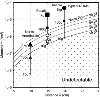
FIG. 5. Detection limits of the magnetometer for different sensor noise floors (15 pT, 30 pT, 60 pT, and 90 pT).The solid lines indicate
493
where the peak-to-peak intensity of the sinusoidal signal by a rotation of a dipole moment m observed at distance d becomes equal to
494
the given noise intensity. Note that the inclination of the dipole is horizontal making the largest amplitudes. The magnetic moment at
495
the hatched region is undetectable due to the weak signal below noise floor of the sensor. The calculated intensities of natural remanent
496
magnetizations (NRMs) of different masses and types of moon rocks are also shown. The NRMs of the moon rocks are given by a
497
previous study 6. The samples measured in this study are also shown (a = 12018.15 at NASA, b = StdBlockNo13 at CEREGE;
498
measurements data shown in figures 3 and 4, respectively).
22
500
FIG. 6. (a) The half-cycle of the calculated signals according to Helbig 23, expressed as linkage coefficient for the radial
501
and tangential components. The distance (r) equals to the length of the edge of the cube (a). The sinusoidal curves
502
indicate the signal from dipole source and the M-shaped deformed curve is the signal from a cubic homogeneously
503
magnetized sample. The difference between the signal from the cube and the dipole source becomes maximum at the
504
peak of the sinusoidal curve (0° for the radial component and 90° for the tangential component). (b)The maximum error
505
normalized by the amplitude of the dipole field (normalized error) as a function of the distance normalized by the length
506
of the edge (r/a). A fitting curve is also shown. The inset of (b) shows the geometry of the samples and the sensor.
507
508
23
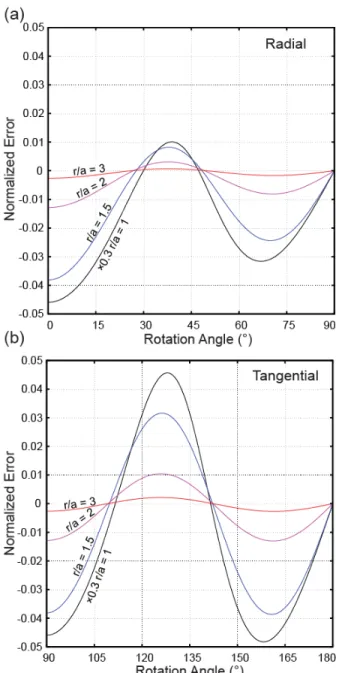
509
510
FIG. 7.The errors due to the shape effect of a cubic-shaped sample at different normalized sensor-to-sample distances (r/a).The ranges
511
of the rotation angle are limited to quarter cycles from the peak position of the dipole field (0° for the radial component, a; 90° for
512
the tangential component, b). The values are normalized by the amplitude of the dipole field. The curves for r/a = 1 is reduced to
513
0.3 of the original curves.
514
515
24
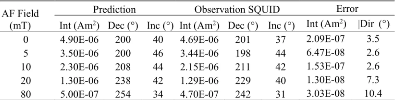
TABLE 1. Alternating field (AF) demagnetization result of StdBlockNo13, showing intensity, declination, and inclination obtained by
516
the prediction given by the inversion results of the developed spinner magnetometer and the observation by the SQUID magnetometer.
517
The intensity and angular errors (|Dir|) between the predictions and the SQUID vector moments are also shown. The angular error is in
518
absolute values.519
520
AF Field
(mT)
Prediction Observation
SQUID
Error
Int (Am
2) Dec (°) Inc (°) Int (Am
2) Dec (°) Inc (°) Int (Am
2) |Dir|
(°)
0 4.90E-06
200
40
4.69E-06
201
37
2.09E-07 3.5
5 3.50E-06
200
46
3.44E-06
198
44
6.47E-08 2.6
10 2.30E-06
208
44
2.15E-06
211
42
1.53E-07 2.6
20 1.30E-06
238
42
1.29E-06
229
40
1.30E-08 7.3
80 5.00E-07
254
34
4.70E-07
242
31
3.03E-08 10.4
521
522
523
TABLE 2. A result of repeated measure of sample StdBlockNo13, showing intensity, declination, and inclination obtained by the
524
prediction given by the inversion results. The mean value, the standard deviation, the semi-angle of aperture of the 95% confidence
525
cone (α95) and the angular standard deviation (θ65) of the magnetic moment vectors are also shown.
526
527
#Run Int
(Am
2) Dec (°) Inc (°)
1 8.95E-05 2.5 1.5
2 9.37E-05 0.1 2.3
3 9.61E-05 1.4 0
4 9.53E-05 0.6 2.1
5 9.39E-05 0.7 3.8
Mean 9.37E-05 1.1
1.9
Stdev 2.56E-06
-
-
α
95-
1.8°
θ
65-
2.1°
528
529
530
531
532
TABLE 3. Result of measurement of sample StdBlockNo13 at different sensor-to-sample distance, showing intensity, declination, and
533
inclination obtained by the prediction given by the inversion results. The mean value, the standard deviation, the semi-angle of
534
aperture of the 95% confidence cone (α95) and the angular standard deviation (θ65) of the magnetic moment vectors are also shown.
535
536
Distance (mm) Int (Am
2) Dec (°) Inc (°)
80 9.47E-05
-0.5
-91.3
100 9.29E-05
0.1
-91.8
130 9.54E-05
1.1
-91.6
160 1.01E-04
1.8
-94.0
Mean 9.59E-05
0.5
-92.4
Stdev 3.36E06
-α
95- 1.7°
θ
65- 2.2°
537
538
539
550mm
1
5
4
3
2
6
500mm
7
8
13
14
11
12
10
9
(a)
(b)
Y
X
Z
X
Z
Y
FG
Encoder Index
Signal Conditioning Unit (SCU3) X Y Z 2ndorder LPF 100 Hz G=1000 AMP 1storder LPF 100 Hz X Y Z ×3Ch 3 Ch 24bit ADC Simultaneous NI 9239
d
Phase A Phase B INDEX Position = 0 ~ 511 Resolution 360/512° Pa ra lle l I/ O NI 9403 8 De co de r PC LabVIEW USB Oversampling 50 ksps × 3ch Read Encoder Save Show Data Post-processing 50 Hz trigger RT Main Loop Software diagram U SB Ch ass is N Ic DA Q -917 4 50 sps × 3ch Position θ θ = 0 toward the FG Synchronize - Position - Field (nT) - Time (ms) Averaging 1k Sampl. Stage North Notch 510 511 0 1 2 BY BX BZ 0° θ mx mz myOriginal Signal
Angle (°) 1tick = 740° Angle (°) 1tick = 740°
(a)
(b)
(c)
(nT) (nT) (nT)+4.5% +2.0% +7.0% +0.8% +6.4% 0.0E+0 1.0E-6 2.0E-6 3.0E-6 4.0E-6 5.0E-6 0 20 40 60 80 100 M ag ne tic M om en t ( Am 2) AF Demagnetizing Field (mT) AF Demag - StdBlockNo13 (w = 0.98 g) Predicted SQUID
(a)
(b)
Mo me n t m (Am 2) Distance d (cm) 1e-9 1e-8 1e-7 1e-6 1e-5 1e-4 5 10 15 20 25 30 Breccia Basalt 1kg 1kg 100g 100g 100g 10g 10g 10g
Undetectable
Norite, Anorthosite Typical NRMs 60 pT 30 pT 1kg b a Noise Floo r = 90 pT 15 pT0 0.5 1 1.5 2 -90 -45 0 45 90 0 0.25 0.5 0.75 1 0 45 90 135 180 Rotation Angle (°) Linkage Coef ficient (dimentionless) Radial Tangential
Distance r = 1 cube a = 1 dipole
(a)
(b)
1e-4 0.001 0.01 0.1 1 1 1.5 2 2.5 3 3.5 4 4.5 5Normalized Distance r/a
Normalized Error radial tangential fitting y = 0.178 x-3.852 sensor r a y x
×0.3 r/a = 1 r/a = 1.5 r/a = 2 r/a = 3 -0.05 -0.04 -0.03 -0.02 -0.01 0 0.01 0.02 0.03 0.04 0.05 0 15 30 45 60 75 90 Rotation Angle (°) Normalized Error -0.05 -0.04 -0.03 -0.02 -0.01 0 0.01 0.02 0.03 0.04 0.05 90 105 120 135 150 165 180 Rotation Angle (°) Normalized Error ×0.3 r/a = 1 r/a = 1.5 r/a = 2 r/a = 3 Radial Tangential