HAL Id: hal-03009570
https://hal.archives-ouvertes.fr/hal-03009570
Submitted on 14 Dec 2020
HAL is a multi-disciplinary open access
archive for the deposit and dissemination of
sci-entific research documents, whether they are
pub-lished or not. The documents may come from
teaching and research institutions in France or
abroad, or from public or private research centers.
L’archive ouverte pluridisciplinaire HAL, est
destinée au dépôt et à la diffusion de documents
scientifiques de niveau recherche, publiés ou non,
émanant des établissements d’enseignement et de
recherche français ou étrangers, des laboratoires
publics ou privés.
Spectroscopy Observations. I. H ii Region Kinematics
Carter Rhea, Laurie Rousseau-Nepton, Simon Prunet, Julie
Hlavacek-Larrondo, Sébastien Fabbro
To cite this version:
Carter Rhea, Laurie Rousseau-Nepton, Simon Prunet, Julie Hlavacek-Larrondo, Sébastien Fabbro. A
Machine-learning Approach to Integral Field Unit Spectroscopy Observations. I. H ii Region
Kinemat-ics. The Astrophysical Journal, American Astronomical Society, 2020, 901 (2), pp.152.
�10.3847/1538-4357/abb0e3�. �hal-03009570�
Canada-France-Hawaii Telescope, Kamuela, HI, United States
3NRC Herzberg Astronomy and Astrophysics, 5071 West Saanich Road, Victoria, BC, V9E 2E7, Canada 4Department of Physics and Astronomy, University of Victoria, Victoria, BC, V8P 5C2, Canada
(Received June 1, 2019; Revised January 10, 2019; Accepted August 26, 2020)
Submitted to AJ ABSTRACT
SITELLE is a novel integral field unit spectroscopy instrument that has an impressive spatial (11 by 11 arcmin), spectral coverage, and spectral resolution (R∼1-20000). SIGNALS is anticipated to obtain deep observations (down to 3.6 × 10⁻¹⁷ergs s−1cm−2) of 40 galaxies, each needing complex and substantial time to extract spectral information. We present a method that uses Convolution Neural Networks (CNN) for estimating emission line parameters in optical spectra obtained with SITELLE as part of the SIGNALS large program. Our algorithm is trained and tested on synthetic data representing typical emission spectra for HII regions based on Mexican Million Models database (3MdB) BOND simulations. The network’s activation map demonstrates its ability to extract the dynamical (broadening and velocity) parameters from a set of 5 emission lines (e.g. Hα, N[II] doublet, and S[II] doublet) in the SN3 (651-685 nm) filter of SITELLE. Once trained, the algorithm was tested on real SITELLE observations in the SIGNALS program of one of the South West fields of M33. The CNN recovers the dynamical parameters with an accuracy better than 5 km s−1in regions with a signal-to-noise ratio greater than 15 over the Hα line. More importantly, our CNN method reduces calculation time by over an order of magnitude on the spectral cube with native spatial resolution when compared with standard fitting procedures. These results clearly illustrate the power of machine learning algorithms for the use in future IFU-based missions. Subsequent work will explore the applicability of the methodology to other spectral parameters such as the flux of key emission lines.
1. INTRODUCTION
HII regions lay the foundation of many studies from star-formation in galaxies, to galactic evolution and cos-mology, and are one of the main drivers of observational extra-galactic astronomy (e.g. French 1980; Weedman et al. 1981; Veilleux & Osterbrock 1987). HII regions form when the gaseous clumps are irradiated by an inte-rior young and hot star or cluster of stars causing the gas to become partially or completely ionized (e.g. Oster-brock & Ferland 1989;Shields 1990;Franco et al. 2000). They are primarily composed of Hydrogen and Helium, but contain non-negligible amounts of metals and their
Corresponding author: Carter Rhea
carterrhea@astro.umontreal.ca
ionized counterparts (e.g. Shields & Tinsley 1976; Oey & Kennicutt 1993; Kennicutt & Oey 1993; Garnett & Shields 1987). The characteristic bright emission lines coming from recombination and collision between the free electrons and the different atoms/ions in the nebu-lae are observed at large distances and allow the study of interstellar matter and its primary constituents (e.g. Kewley et al. 2006;Crawford et al. 1999;Baldwin et al. 1981). Additionally, the omnipresence of the HII regions in some galaxies allow for the study of galactic disk dy-namics (e.g. Epinat et al. 2008), magnetic fields and turbulence at large and small-scales (e.g. Odell 1986; Haverkorn et al. 2015; Beck et al. 1996; Quireza et al. 2006; Pavel & Clemens 2012), and the importance of various feedback mechanisms that inject energy into the ISM, i.e. stellar winds, supernovae and radiation
sure (e.g. McLeod et al. 2020; Ramachandran et al. 2018,2019).
More recently, the use of integral field spectroscopy on nearby galactic and extragalactic HII regions has offered a more complete view of their physical properties (e.g. Leroy et al. 2016;Snchez et al. 2012;Bundy et al. 2014). Also, increasing spectral and spatial resolution has al-lowed for the study of the complex dynamical structures of the HII regions and pushed the limit of previous anal-ysis methods meant for integrated/unresolved spectra of HII regions (e.g. Martins et al. 2010;Snchez et al. 2012; Drissen et al. 2014). Typical fitting procedures used to extract the dynamics and emission lines flux measure-ments from HII regions spectra require a good prior es-timate of the velocity as well as the number of velocity components to be fitted (e.g. Zeidler et al. 2019;Bittner et al. 2019; Snchez et al. 2007). Defining the range of those priors is usually not a problem when the ensem-ble of spectra shows similar characteristics. While the typical range of velocity seen in galactic disks can easily vary by a few hundreds of km s−1(e.g. Dressler et al. 1983;Bregman 1980;Sancisi et al. 2008), and the inter-nal dynamics of HII regions can add thermal/turbulent broadening and expansion velocity to the galactic con-tribution (e.g. SOFUE 1995;Arsenault 1986), the typ-ical velocity prior for a given spectral data cube can be very broad and is often not precise enough to ensure a proper fit of the entire data set. We are additionally facing new challenges in the dynamical analysis, because the spatially resolved HII regions spectra often contain emission from different phases of the ISM (along the line of sight) and can be composed of multiple dynamically distinct components (e.g. expanding shells,Rozas et al. 2007; Relao & Beckman 2005) having each a different thermal/turbulent broadening. Of course, fitting two or more components with the proper velocity and broad-ening priors is the best approach in such case, but only when such components are actually present in the spec-tra (e.g. Relao et al. 2005;Le Coarer, E. et al. 1993).
Ultimately, extracting the information in a consistent manner from high spectral and spatial resolution data cubes requires a dedicated method to estimate the priors on the different spectral parameters, taking into account the variation of the observed spectral features across the field-of-view.
SITELLE, the Imaging Fourier Transform Spectro-graph (IFTS) of the Canada-France-Hawaii Telescope (CHFT), produces spectral data cubes containing over 4 million pixels with adjustable resolving power (up to 10,000) and has an instrumental line shape described by a sine cardinal function (Martin & Drissen 2017; Baril et al. 2016;Drissen et al. 2019). Its 110× 110
field-of-view (FOV) contains more than 4 million pixels for which the spectral sampling and resolution varies as a function of their relative position angle with the mobile mirror. Moreover, emission lines intensities (and there-fore line intensity ratios) may vary significantly across the parameter space of the physical properties observed in HII regions.
All together, these characteristics make a typical tem-plate fitting strategy (e.g. cross-correlation function maximization) very difficult to implement since the sine cardinal function side lobes affect neighbouring line in-tensity and shape, and the position of the lobes with respect to the central position of the line varies with spectral resolution (changes across the FOV). In addi-tion, the variation of line intensity ratios between dif-ferent emission regions can lead to gross errors on the velocity estimates when a single template spectrum is used. Therefore, an adapted approach is developed here to solve these issues while still fitting entire data cubes, using the same uniform and reproducible method and including the dynamical and spectral complex nature of the resolved HII regions.
This paper explores the use of a Convolution Neu-ral Network to resolve deficiencies in the existing fitting software ORCS – Outils de R´eduction de Cubes Spectraux. Although the ORCS fitting routines are robust, they re-quire a human-generated prior for all fits; this paper demonstrates the use of machine learning to estimate the priors with no human input. In § 2, we outline the Convolution Neural Network and the synthetic data set used to train the network. We explore the success of our CNN to the synthetic data in § 3. In § 4, we discuss the applicability of our methodology to low resolution spec-tra. Additionally, we apply the CNN to a field of M33 in order to test its efficacy in real observations. Finally, in § 5, we recap the main successes and outline our future work.
2. METHODOLOGY
2.1. Convolutional Neural Networks
Neural Networks have been used extensively in astron-omy to classify galaxies (Storrie-Lombardi et al. 1992), separate galaxies from stars (Bertin 1994), categorize dynamic parameters of galaxy clusters (e.g. Ntampaka et al. 2016; Ntampaka et al. 2019), explore astrophys-ical morphologies at differing scales (e.g. Sadaghiani et al. 2019; Iwasaki et al. 2019), derive galaxy redshift from wide band images (Pasquet et al. 2019), and ex-tract emission-line parameters from spectra (e.g. Olney et al. 2020; Ucci et al. 2019;Baron 2019). A recent ef-fort to calculate the parameters of HII regions from their
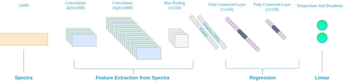
Figure 1. A cartoon of the convolutional neural network used in this work. As described in the text, it is an adaptation of the STARNET topology (Fabbro et al. 2018). The input spectra is first convolved in two separate layers before being condensed in a pooling layer. Once flattened, the vector is passed to two hidden layers. Finally, the velocity and broadening parameters are estimated using two separate output nodes denoted by the blue-green bar.
spectra, GAME1, employs a combination of Decision Trees and AdaBoost in order to predict physical parameters (Ucci et al. 2017; Ucci et al. 2018). In lieu of this, our method uses a Convolutional Neural Network (CNN) ar-chitecture designed by Fabbro et al.(2018), monikered STARNET, which has already demonstrated success in es-timating emission-line parameters from stellar spectra.
During the course of this work, we became aware of the work ofKeown et al.(2019), which uses an approach similar to ours to estimate the velocity and broaden-ing of high resolution radio emission lines, takbroaden-ing into account possible multiple velocity components. While their work focuses on high resolution, isolated emission lines, ours focuses on lower resolution spectra observed on a wide field of view, hence often with a wide veloc-ity distribution. In addition, the SITELLE ILS extended structure prevents us in any case from considering the different emission lines separately.
Our convolutional neural network is graphically de-picted in figure1and laid out as follows:
1. 8x8 convolution with 4 filters 2. 4x4 convolution with 8 filters 3. Global max pooling with 4 filters 4. 20% dropout
5. 256 fully-connected nodes 6. 128 fully-connected nodes 7. 2 output neurons
The CNN takes the normalized SITELLE emission spectra obtained with the SN3 filter (651-685 nm) and returns an estimate on the velocity (km s−1) of the lines and their broadening (km s−1), assuming they are
1https://game.sns.it/
consistent over the five major emission lines in SN3. We tested several scaling functions (RobustScaler, Stan-dardScaler, and MinMaxScaler); although we obtained the tightest constraints with the MinMaxScaler, the ac-tivation map revealed fitting nonphysical features and noise. We therefore normalize the spectrum to have a maximum value equal to unity.
In order to ensure the appropriate hyper-parameters, we explored their spaces extensively using the random search algorithm, as implemented by sklearn, embed-ded in a 10-fold cross correlataion. Throughout our training, we saw no significant deviation from the re-sults reported by Fabbro et al. (2018). Therefore, we adopted the same hyper-parameter values as used in the standard STARNET procedure. Structural hyper-parameters can be readily seen in figure 1. In order to view the other parameters (i.e. learning rates, decay rates, etc.), we suggest the reader view our github page: https://github.com/sitelle-signals/Pomplemousse. We report a maximum number of 10 epochs and an initial batch size of 8 spectra.
2.2. Synthetic Data
In order to demonstrate the feasibility of using a CNN to identify the correct spectral parameters, we construct a set of synthetic data on which to train and test the network. The synthetic data set used in this study was created using the ORB software de-veloped to reduce data from SITELLE (Martin et al. 2016). To generate synthetic spectra, We use the ORB create cm1 lines model function which requires a number of parameters that will be defined in this section. Since our tool was developed primarily for SITELLE’s programs and the SIGNALS collaboration, we focused on the SN3-filter which covers a band pass between 647 and 685 nm. In accordance with the SIGNALS sur-vey, we select a primary spectral resolving power of 5000, an exposure time of 13.3s per step, and 842 steps (Rousseau-Nepton et al. 2019). In order to replicate
the change of spectral resolution across the cube, we al-low the resolving power to randomly vary between 4800 and 5000 since the resolution will vary between these values in any given SN3 observation which is a part of the SIGNALS program. We will model the following lines: [NII]λ6548, Hα(6563)˚A, [NII]λ6583, [SII]λ6716, and S[II]λ6731. Furthermore, we use the sincgauss function as described inMartin et al.(2016) to include line broadening. We randomly varied the velocity be-tween -200 and 200 km s−1, while the broadening was randomly varied between 0 and 50 km s−1. These ranges were selected from our prior knowledge of the distribu-tion of velocities in M33 (Epinat et al. 2008) and the typical broadening in SITELLE data cubes at this spa-tial resolution. Note that we randomly selected the res-olution, broadening, and velocity parameters with re-placement for each synthetic spectrum. The final input required to construct the synthetic spectra is the ampli-tude of each emission line.
In order to calculate reasonable relative fluxes for the five lines while ensuring we are sampling the desired physical parameter space, we used the 3MdB2 – Mexi-can Million Models Database (Morisset et al. 2015). The 3Mdb contains models created using the CLOUDY v17.01 photoionization code based on a pre-selected set of emis-sion region parameters and underlying ioinizing stellar spectra (Ferland et al. 2017). We use the BOND dataset described in Asari et al. (2016) which contains spectra from HII regions similar to those expected to be found in SIGNALS. The BOND data-set contains 63000 spec-tra. Though the data set covers the physical parameter space of the emission nebulae we wish to study, it also contains a number of models that are outside the scope of our study. We describe varying parameters used in table1. While the BOND simulations have two simulation geometries, completely filled and thin shell, we remove all thin shell (fraction=0.03) simulations from our sam-ple. This leaves us with filled spheres with a density of approximately 100 cm3 and represents a younger
pop-ulation of HII regions (e.g. Asari et al. 2016; Stasiska et al. 2015;Cedrs et al. 2013).
We further constrained the ionization parameter, U, and metallicity proxy, 12+log(O/H), to focus on SIGNALS-type HII regions (e.g. Rousseau-Nepton et al. 2019;Prez-Montero et al. 2019; Kashino & Inoue 2019; Zinchenko et al. 2019). With these constraints, we ex-tracted the amplitudes of the five emission lines present in SN3, first randomly selecting a model which passed our selection criteria. We then normalized the
ampli-2https://sites.google.com/site/mexicanmillionmodels/
Parameter Lower Limit Upper Limit Step Size log(U) -3.5 -2.5 0.5
Age (Myr) 1 6 1
12+log(O/H) 7.4 9.0 0.2
log(N/O) -2 0 0.5
Table 1. HII region parameter selection used during the M3db runs of the BOND simulations. The initial run-parameters were cut further in order to focus on the emission expected in the SIGNALS program. The step sizes were set by the 3Mdb runs (seeMorisset et al.(2015) for more infor-mation)
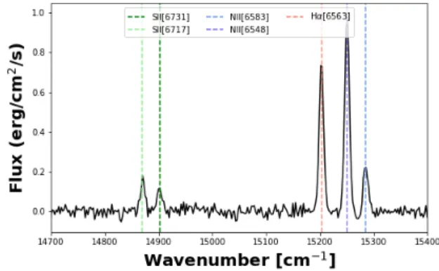
tudes with respect to Hα. After combining the five lines (with the appropriate instrumental line shape) and the simulated continuum emission, we add a noise compo-nent. The SNR is sampled from a uniform distribution between 5 and 30. Below a SNR of 5, the lines are nearly indistinguishable and the sidelobes of the ILS are com-pletely obstructed. We expect a nominal high (> 20) SNR for Hα in the SIGNALS program. SNR effects will be investigated later in the article. Figure 2 shows a sample spectrum. At this stage, we create 50,000 mock spectra in the form of FITS files which contain the emis-sion parameter information (e.g. velocity, broadening, resolution).
Figure 2. Example spectrum simulated using the process described in §2.2. As our population statistics suggest, this is not the only expected spectral shape. However, it is rep-resentative of the sample and clearly demonstrates the five emission line peaks. This is the SN3 spectral coverage of SITELLE.
2.3. SITELLE Data
2.3.1. Calibration and Data Reduction
Observations of M33 were taken during the Queued Service Observing period 18B (Program 18BP41, P.I. Laurie Rousseau-Nepton) at the Canada France Hawaii Telescope on the summit of Mauna Kea, Hawaii, using
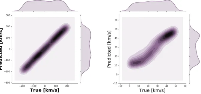
Figure 3. Kernel Density Estimation (KDE) plots for the test set. Left: True vs Predicted Velocity values in km s−1. Right: True vs Predicted Broadening values in km s−1. In both plots we can see that the predicted values accurately mimic the true values. Note the change in scales between the two plots.
Figure 4. Left: Velocity Residual as a function of the true velocity. Although there exists a background substructure, it only affects a fraction of a percent of the total test set and is thus negligible. Right:Broadening residual as a function of the true broadening. The pattern demonstrates a bias for low broadening values that is likely caused by the networks inability to distinguish a low amount of broadening. Moreover, the broadening naturally segregates itself into two physical peaks typical of HII regions and supernovae remnants, respectively (e.g. Veilleux & Osterbrock 1987;Vasiliev et al. 2015).
SITELLE. These exposures were taken with the SN3 fil-ter which covers a range from 651-685 nm for a total of 4h with a spectral resolving power of R∼5000. The pointing was centered on a single field in M33 and is part of a larger observation of M33 in its entirety. This ob-servation also forms a basis for the SIGNALS program, lead by Laurie Rousseau-Nepton, which aims to further categorize HII and star-forming regions in nearby galax-ies. We note that the authors of this paper are members of the SIGNALS collaboration.
The raw data were reduced and calibrated us-ing SITELLE’s personalized software, ORBS (ver-sion 3.1.2 Martin et al. 2016). We are able to
re-solve five spectral emission lines from our observations: [SII]λ6713, [SII]λ6731, [NII]λ6548, Hα, [NII]λ6584. Us-ing the function SpectralCube.Map Sky Velocity(), we fit the OH sky line velocities, assumed at rest w.r.t. the observer, with a geometric model of the interferometer; afterwards, we used the func-tion SpectralCube.Correct Wavelength() to refine the wavelength calibration of our data cube using the OH-lines fit.
3. RESULTS
In this section we apply our convolutional neural net-work outlined in §2.1 to our synthetic spectra with a resolution R∼5000. We retained 70% (35,000) of the
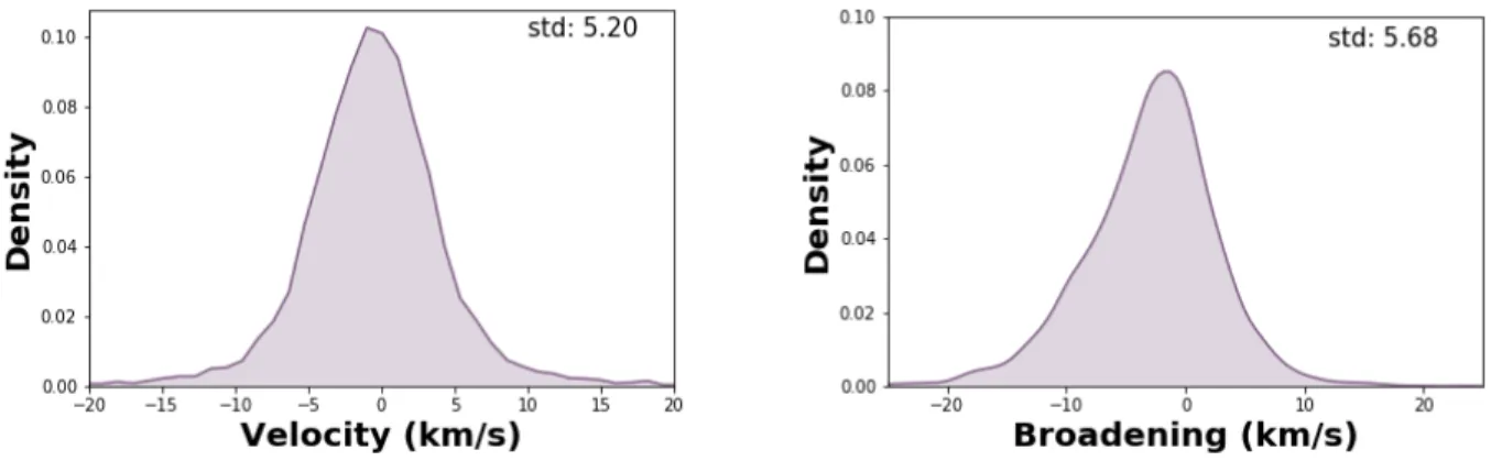
Figure 5. Left: Density plot of the velocity residuals in km s−1along with the standard deviation. Right: Density plot of the broadening residuals in km s−1in addition to the standard deviation. The asymmetry is likely due to the diversity of resolving power introduced in the training set.
Figure 6. Activation or Saliency Map of our convolutional neural network applied to an example spectrum. The colored points represent the exact locations of the nodes in the input spectrum. Their color indicates their relative weight in the network. Weights under 0.25 are not shown for clarity.
spectra as our training set, 20% (10,000) as our vali-dation set, and the remaining 10% (5,000) as the test set (e.g. Tetko & Villa 1997). Training and validat-ing our algorithm results in over 95% accuracy for both predicted parameters: the velocity and the broadening. Accuracy is defined as the ratio of correct parameter estimations to the total number of estimates. An esti-mate is considered correct if it agrees with the ground truth value up to two digits after the decimal (i.e. to the hundredth place). The combined mean absolute error, another common metric for regression tasks, is 5kms−1.
Figures 3, 4, and 5 visually depict the accuracy of the CNN on the test set and the associated residuals, re-spectively. As the figures depict, the algorithm was well trained and is able to accurately predict both the veloc-ity and the spectral broadening. As evidenced in figures 3 and 4, the predicted values are close to the ground truth values. The KDE plots in figure 3 demonstrate that the parameter space is being well sampled for both
the velocity and broadening. Figure5demonstrates the Gaussian distribution of errors about zero; although the right panel reveals the slightly skewed error distribu-tion of the broadening parameter, the shape is globally Gaussian and any distortion is believed to be caused by asymmetries within the training set. We report a stan-dard deviation of ∼ 5 km s−1for the velocity parameter. This is well within the required limits as described in Martin et al.(2016) andRousseau-Nepton et al.(2019) for an initial guess to be supplied to the ORCS software. The velocity error is required to be less than the channel width with corresponds to approximately 40 km s−1for a resolution of 5000. The standard deviation of the broad-ening parameter is ∼ 5.5 km s−1. Since SITELLE re-solves the broadening parameter down to approximately 3 km s−1for high SNR regions (∼1000), our broadening errors are near SITELLE’s resolving power.
In order to compare the network results to those re-covered by the ORB/ORCS software, we fit the test set using the fit lines in spectrum routine. The veloc-ity and broadening parameters were initialized as the precise velocity and broadening parameters used to con-struct the spectra. Although this is improbable to occur during a standard fitting procedure, hence the need for an accurate estimate, this demonstrates the best pos-sible case for the fitting algorithm. All other param-eters were also set to those used to simulate the spec-tra. The fitting procedure recovers the true velocity with a standard deviation of ∼ 3km s−1and the broadening with a standard deviation of ∼ 4km s−1. Comparing these standard deviations with those from the CNN, we note that the ORB/ORCS recover the true parameters with marginally better accuracy.
Although the spread of errors shown in the figures 5 and4do not reveal overt overfitting, we applied a stan-dard k-fold cross-validation algorithm on ten partitions of the training, validation, and test data (e.g. Picard
taining the same test set. We report approximately the same accuracy values (within 5%) regardless of the fold and cross-validation technique. This further indicates the absence of overfitting (e.g. Cawley & Talbot 2010; Molinaro et al. 2005).
Additionally, we created an saliency map of our ex-ample spectrum from figure 2 which can be seen with the filled circles in figure6. The saliency map delineates the regions of the input (in this case the spectrum) used by the convolutional neural network to learn (e.g. Si-monyan et al. 2014) by calculating the gradient of the output with respect to the input. More precisely, the map is created by varying one input variable at a time and calculating the change in the loss function. In this manner the algorithm highlights the most important in-put nodes. We can clearly see by the clustering of data points in the image around the Hα and [NII]λ6548 lines that the network considers these lines to be the most important components for determining the velocity and broadening. This is consistent with our expectations since these two lines, unlike the others, are consistently above the continuum in HII regions. It is sensible that the network does not weigh the [SII] doublet heavily since they are often unobservable due to noise. More-over, the network does not focus only on the peaks of the Hα and [NII]λ6548 lines, but also on their base. This indicates that the widening of the lines – which is directly affected by the velocity and broadening compo-nents – plays a crucial role in parameter estimation, as expected.
4. DISCUSSION
While in Section 3, we demonstrated that the CNN algorithm is capable of extracting the correct spectral parameters (velocity and broadening) of the Hα, N[II], S[II] lines for synthetic SITELLE observations, in this Section, we examine the versatility of the model and its robustness when applied to real SITELLE observations. We also discuss the novelty of using such CNN algo-rithms for IFU observations in general (i.e. from other telescopes, especially in context of upcoming 30 and 40 -m class telescopes.
4.1. Versatility of the Model
R∼2000, we wished to directly test our existing network and weights against synthetic data created with R∼2000 (e.g. Puertas et al. 2019;Gendron-Marsolais et al. 2018; Rousseau-Nepton et al. 2018). However, since the reso-lution sets the number of steps (i.e. data points) in our spectrum, a reduction of the resolution affects the length of the input data. In order to feed lower resolution spec-tra into our CNN, we would be required to smooth or interpolate the data so that we would have an input of an equivalent length – a requisite for use in a CNN. In doing so, we would be assuming a form of the interpolation (i.e. linear, a higher-order polynomial, spline, etc.) which might inject non-physical and potentially biased infor-mation into the spectra (Horowitz 1974; Scargle 1982; Schulz & Stattegger 1997). We therefore do not mod-ify the spectra, but instead we create an entirely new set of training, validation, and test data using the same routines employed to create our high spectral resolution synthetic dataset with a resolution set to R∼2000.
After creating 30,000 synthetic spectra with a lower spectral-resolution, we divided the set into the train-ing (70%), validation (20%), and test (10%) sets. Af-ter training and validating our convolutional neural net-work, we applied it on our test data. We report a nom-inal accuracy of both predictors (velocity and broad-ening) of 92% compared to 95% in the case of R∼5000. The standard deviation of the errors for the velocity and broadening are 75 and 12 km s−1, respectively. We ran both k-fold cross-validation algorithms and again found consistency across the accuracy predictors. The re-sults are coherent with our supposition that the method would extend well to relatively low resolution spectra since, even at R∼2000, we are able to reasonably resolve the emission lines. The reduced accuracy is reasonable since the emission lines are less well-resolved.
We attempted to use the network to predict low res-olution SITELLE spectra (R∼1000); however, at this resolution, the lines are often indistinguishable and the algorithm fails to achieve high-fidelity results. Typ-ical SITELLE’s observing strategy for targets in the local Universe and for the SIGNALS project, have an increased spectral resolution for the Hα filter (SN3) and often a lower resolution for other filters (typically R∼1000). The dynamical priors (velocity and
broad-ening) can then be estimated using the higher resolu-tion SN3 filter and applied on the other observaresolu-tions of the same field with the other filters. Overall, our re-sults demonstrate that a CNN network is capable of reliably estimating spectral parameters (velocity and broadening) in SITELLE synthetic observations at high (R=5000) and low (R=2000) resolution, but that be-yond R = 1000-1500, it fails because of the poor quality of observations. In other words, these results not only demonstrate that machine learning algorithms can be used to estimate kinematic parameters, but they also demonstrate the techniques limitations.
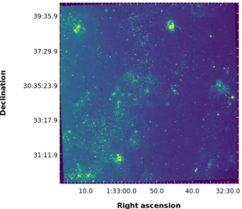
4.2. Validation on a real data-set: the case of M33 With the ability of the CNN to predict velocity and broadening parameters accurately for synthetic data, we apply our methodology to an emission region of M33’s South-East field (figure 7). This region is an excellent test-bed for our algorithm since it contains several types of emission regions (i.e. HII region, planetary nebulae, etc.) and is part of the SIGNALS survey.
Figure 7. Deep, co-added SITELLE observation (4hr) of M33 Field 7 using the SN3 filter. The image illustrates the density of emission-line regions in the outskirts of M33.
Fits were calculated using the ORCS
fit lines in region() command centered on our five lines. Each grouping ([SII]λ6713/[SII]λ6731, [NII]λ6548/[NII]λ6584, and Hα) was fit simultaneously with a Gaussian convolved with a sinc function fol-lowing the standard SITELLE procedure (Martin & Drissen 2017); All lines were tied together with respect to the velocity and broadening. Fits were optimized using the Levenberg-Marquardt least-squares minimiza-tion algorithm. In order to execute a fit in ORCS, the
user is required to input an initial guess for the velocity and broadening parameters; this is due to the nature of the minimization algorithm. The first set of priors were created by initially binning our cube into spatial bins of 8x8 followed by the standard ORCS fitting procedure. This standard method still requires an initial guess that the user must input. However, the machine learning method for determining priors does not require any user input and can be applied directly on the unbinned data. All fits were run using a computing server located at the CFHT headquarters in Waimea, Hawaii named iolani. The server has 2 Intel XEON E5-2630 v3 CPUs operating at 2.40GHz with 8 cores each. The configu-ration also has 64 GB of RAM available for computing purposes.
A key benefit of the machine learning prior fits over the standard procedure is the economy of time asso-ciated with the machine learning algorithm. Since no fitting and iterating is necessary, the calculation time scales approximately linearly with the number of spec-tra. Using a coarse initial binning, 8x8, the standard algorithm to calculate the priors takes approximately 4 hours in order to cover the entire cube. However, the un-parallelized machine learning algorithm takes only 180 seconds3to cover the same binned cube. Hence the ma-chine learning algorithm calculates the priors more than 100 times faster than the standard algorithm. We also calculate the time the machine learning algorithm takes to estimate the velocity and broadening parameters for an unbinned cube; this takes approximately 4 hours – the same amount of time to calculate the standard priors on an binned (8x8) cube.
In addition to being considerably faster when esti-mating the priors, the machine learning algorithm also obtains accurate estimates. In order to quantify this notion, we calculate the residual values over the cube between the unbinned final fits – using an 8x8 machine learning prior – and the unbinned machine learning esti-mates. We only retained pixels for the residual analysis which demonstrated a flux value above our threshold of 2 × 10⁻¹⁷ ergs/s. This threshold was chosen since it masks out all nan values and maintains the regions with clear emission. Figure8demonstrates that the residuals are low in central parts of the emission regions, where the signal-to-noise is high, while the residuals are higher in the outskirts where the signal-to-noise is low. This is likely due to the fact that our synthetic data was created using a high signal-to-noise ratio of 50; we will explore
3assuming a near-perfect speedup, we expect the parallelized
Figure 8. Left: Residual map of the velocity calculated from the absolute difference between the final ORCS fit and the machine learning priors calculated on an unbinned cube. Right: Residual map of the broadening calculated from the absolute difference between the final ORCS fit and the machine learning priors calculated on an unbinned cube. Both maps were smoothed using a 2-dimensional Gaussian kernel with a sigma value equal to 2 pixels.
the effects of the SNR ratio in a future paper. While it is often desirable to study the emission in the outskirts in addition to the central emission, the low-residual re-gions outline locations of high-fidelity fits. In order to recover the velocity and broadening parameters in these regions, the machine learning estimates on either the binned or unbinned cube can be used as priors for a standard ORCS fit. Moreover, since the standard prior calculation requires binning spatially, substructure in-formation is inherently lost in these priors. On the other hand, the convolutional neural network priors do not re-quire any binning and thus retain all structural spatial information.
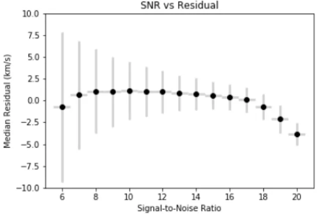
Figure 9. Proxy signal-to-noise ratio versus mean absolute velocity residual (km s−1) for the South West field of M33. For each SNR bin, we excluded outliers before calculating the mean absolute residual and standard deviation (grey y-axis error bars). Each SNR bin has a width of 1.
Figure 10. Proxy signal-to-noise ratio versus mean abso-lute broadening residual (km s−1) for the South West field of M33. For each SNR bin, we excluded outliers before cal-culating the mean absolute residual and standard deviation (grey y-axis error bars). Each SNR bin has a width of 1.
Although we do not study all the complexities of the SNR impact on our CNN in this article, we include a short discussion on it here. We calculate the SNR by di-viding the Hα flux by its fit uncertainty as calculated in our final ORCS fit. Although this is not exactly the SNR, it acts as a proxy value. With the residual maps and the SNR proxy map, we have the residual and signal-to-noise information for each pixel. We then binned residuals by signal-to-noise ratio with a step size of 1 between 5 and 20. Twenty is the maximum value of the SNR proxy and below 5 we do not see any coherent structure in the spectra. We culled outliers that were outside of the 3-σ range. Finally, we calculated the median absolute residual and standard deviation in each SNR bin. As ev-idenced by figure9, the accuracy of the CNN increases as
the signal-to-noise ratio rises, an expected trend. Figure 10 demonstrates that the broadening residual plateaus at a SNR of approximately 12; moreover, the figure indi-cates a discordance between the CNN’s estimations and those obtained from ORCS fits. We believe this behav-ior is due to the presence of multiple emission compo-nents serendipitously located in high SNR regions (see appendix for discussion). Multiple components affect the broadening parameter stronger than the velocity es-timates. Even in standard fitting procedures, this poses a serious issue.
4.3. Universal Applicability
The methodology described in this paper is not lim-ited to SITELLE data cubes. Indeed, the methodology naturally lends itself to any IFU-like data cube in which the observer has access to high-resolution spectral data such as the K-band Multi Object Spectrograph, KMOS (e.g. Sharples et al. 2013), or the Multi Unit Spectro-scopic Explorer, MUSE (e.g. Bacon et al. 2010). Since the machine learning algorithm is able to achieve reason-able estimations of the kinetic parameters (velocity and broadening) in a fraction of the time the standard fitting procedures take, it will play a crucial role in upcoming missions aimed at completing large-scale surveys using IFUs such as the Near-Infrared Spectrograph, NIRSpec (e.g. de Oliveira et al. 2018), on the James Webb Space Telescope and the MEGARA – Multi-Espectrgrafo en GTC de Alta Resolucin para Astronoma – instrument on the Gran Telescopio Canarias (e.g. Paz et al. 2012).
5. CONCLUSIONS
A convolution neural network has been exploited in several astronomical applications ranging from dynamic mass estimates of galaxy clusters (e.g. Ntampaka et al. 2019) to the extraction of spectral parameters (e.g. Fabbro et al. 2018). This work applies a modified STARNET architecture (Fabbro et al. 2018) to high reso-lution (R>2000) SITELLE observations of HII regions in order to estimate the velocity and broadening pa-rameters. Training, validation, and testing the machine learning algorithm with synthetic data integrating the 3Mdb database (Morisset et al. 2015) demonstrates the feasibility of the method. We demonstrate that the al-gorithm fails to predict the spectral parameters for low resolution (R'1000) observations. We believe this is due to the lack of resolved spectral information result-ing in partial blendresult-ing of the main emission lines.
How-ever, above R∼2000, we are able to disentangle the lines better. We apply the convolutional neural network to the Southwest field of M33 to calculate the velocity and broadening priors. Compared to the standard method for computing the priors, our method is over 100 times faster. Additionally, the machine learning algorithm can reliably estimate the emission-line parameters for the en-tire unbinned cube in roughly the same amount of time it takes the standard algorithm to calculate the priors on an 8x8 binned cube.
The work presented here represents the first in a se-ries of articles on the applications of machine learning to SITELLE spectra. In a subsequent article, we will present our work on the effects of the signal-to-noise ra-tio on convolura-tion neural networks and how to mitigate the negative impacts.
We will also demonstrate the applicability of our methodology to calculate the fluxes (and ratios thereof) of emission lines, which will allow for the rapid clas-sification of emission regions through grids of photo-ionization models (e.g. 3MdB). In the third proposed paper of the series, we will describe a machine learn-ing methodology to identify possible multiple, blended components within emission lines.
ACKNOWLEDGMENTS
The authors would like to thank the Canada-France-Hawaii Telescope (CFHT) which is operated by the Na-tional Research Council (NRC) of Canada, the Institut National des Sciences de l’Univers of the Centre Na-tional de la Recherche Scientifique (CNRS) of France, and the University of Hawaii. The observations at the CFHT were performed with care and respect from the summit of Maunakea which is a significant cultural and historic site. C. R. acknowledges financial support from the physics department of the Universit´e de Montr´eal. J. H.-L. acknowledges support from NSERC via the Dis-covery grant program, as well as the Canada Research Chair program.
The progamming aspects of this paper were completed thanks to the following packages of the python program-ming language (Van Rossum & Drake 2009): numpy (van der Walt et al. 2011, scipy (Virtanen et al. 2020), matplotlib (Hunter 2007), pandas (McKinney 2010), seaborn (Waskom et al. 2017), astropy (Collaboration et al. 2018; Robitaille et al. 2013), tensorflow (Abadi et al. 2015, and keras (Chollet 2015).
our already trained network on the synthetic data. Figure 11demonstrates that the network performs well for high
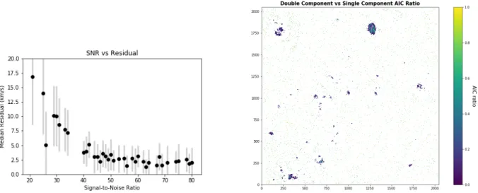
Figure 11. Left: Proxy signal-to-noise ratio versus mean absolute broadening residual (km s−1) for synthetic data created to simulate a range of SNR values. For each SNR bin, we excluded outliers before calculating the mean absolute residual and standard deviation (grey y-axis error bars). Each SNR bin has a width of 1. Right: Ratio of double vs single component AIC parameters for the masked region of interested.
SNR values. Thus the network is not biased for high SNR regions. Note that the SNR value used in this section is the true signal-to-noise ratio as compared to that used in §4.2which is a proxy value calculated by dividing the Hα flux by its fit uncertainty.
In order to determine whether or not the regions of high SNR in the South West field of M33 have single or double emission components, we turn to the standard ORCS fitting procedure. We chose a small region (2x2 pixels) in a high SNR region that also has a large broadening residual (01:32:16.03, +30:48:00.71 ). We selected pixels which fit the following prescription: have a broadening residual higher than 10 kms−1 and a signal-to-noise ratio over 12. We
fit the Hα and NII doublet assuming a single emission component and a double emission component. The double emission fit resulted in a statistically significantly better fit statistic. This is a strong indication that the region is best described by a double emission component rather than a single emission component. Moreover, we computed the AIC parameter for each region defined by AIC = 2n − ln(L), where n is the number of fit parameters and L is the Gaussian likelihood function (e.g. Akaike 1987; Liddle 2007;Kieseppa 1997). In our case, the likelihood is Gaussian, therefore the log-likelihood function reduces to the usual half χ-squared. The right hand-size of figure11shows the ratio of the double component AIC parameter vs the single component AIC parameter defined as exp(−(AIC1− AIC0)/2). Since
the ratio is consistently below one, the double component model is favored over the single component model. We thus conclude that, at least in these regions, the rise in the residual value is due to the existence of double component emission. Therefore, we believe that figure10does not reflect a failure of the network in high SNR regions, but rather a failure of the network in regions with double emission components that serendipitously appear in regions of high SNR in the South West field of M33. Future work will explore the applicability of a modified network to estimate the broadening and velocity parameter in such regions.
REFERENCES
Abadi, M., Agarwal, A., Barham, P., et al. 2015, 19 Akaike, H. 1987, Psychometrika, 52, 317
Arsenault, R. 1986, Astrophysical Journal, 92
Asari, N. V., Stasiska, G., Morisset, C., & Fernandes, R. C. 2016, Monthly Notices of the Royal Astronomical Society, 460, 1739, doi:10.1093/mnras/stw971 Bacon, R., Accardo, M., Adjali, L., et al. 2010, 7735,
773508, doi:10.1117/12.856027
Baldwin, J. A., Phillips, M. M., & Terlevich, R. 1981, Publications of the Astronomical Society of the Pacific, 93, 5, doi:10.1086/130766
Baril, M., Grandmont, F., Mandar, J., et al. 2016, International Society for Optics and Photonics, 990829 Baron, D. 2019, arXiv:1904.07248 [astro-ph].
http://arxiv.org/abs/1904.07248
Beck, R., Brandenburg, A., Moss, D., Shukurov, A., & Sokoloff, D. 1996, Annual Review of Astronomy and Astrophysics, 34, 155,
doi:10.1146/annurev.astro.34.1.155
Bengio, Y., & Grandvalet, Y. 2004, Journal of Machine Learning Research, 1089
Bertin, E. 1994, in Science with Astronomical Near-Infrared Sky Surveys, ed. N. Epchtein, A. Omont, B. Burton, & P. Persi (Dordrecht: Springer Netherlands), 49–51, doi:10.1007/978-94-011-0946-8 11
Bittner, A., Falcn-Barroso, J., Nedelchev, B., et al. 2019, Astronomy & Astrophysics, 628,
doi:10.1051/0004-6361/201935829
Bregman, J. N. 1980, The Astrophysical Journal, 236, 577, doi:10.1086/157776
Bundy, K., Bershady, M. A., Law, D. R., et al. 2014, The Astrophysical Journal, 798, 7,
doi:10.1088/0004-637X/798/1/7
Cawley, G. C., & Talbot, N. L. C. 2010, Journal of Machine Learning Research, 11, 2079
Cedrs, B., Beckman, J. E., Bongiovanni, A., et al. 2013, The Astrophysical Journal, 765, L24,
doi:10.1088/2041-8205/765/1/L24 Chollet, F. 2015, Keras. https://keras.io
Collaboration, T. A., Price-Whelan, A. M., Sipcz, B. M., et al. 2018, The Astronomical Journal, 156, 123, doi:10.3847/1538-3881/aabc4f
Crawford, C. S., Allen, S. W., Ebeling, H., Edge, A. C., & Fabian, A. C. 1999, Monthly Notices of the Royal Astronomical Society, 306, 857,
doi:10.1046/j.1365-8711.1999.02583.x
de Oliveira, C. A., Birkmann, S. M., Boeker, T., et al. 2018, arXiv:1805.06922 [astro-ph].
http://arxiv.org/abs/1805.06922
Dressler, A., Sandage, A., & Wilson, M. 1983, Astrophysical Journal, 265, 664
Drissen, L., Rousseau-Nepton, L., Lavoie, S., et al. 2014, Advances in Astronomy, 2014, 1,
doi:10.1155/2014/293856
Drissen, L., Martin, T., Rousseau-Nepton, L., et al. 2019, Monthly Notices of the Royal Astronomical Society, 485, 3930, doi:10.1093/mnras/stz627
Epinat, B., Amram, P., & Marcelin, M. 2008, Monthly Notices of the Royal Astronomical Society,
doi:10.1111/j.1365-2966.2008.13796.x
Fabbro, S., Venn, K., O’Briain, T., et al. 2018, Monthly Notices of the Royal Astronomical Society, 475, 2978, doi:10.1093/mnras/stx3298
Ferland, G. J., Chatzikos, M., Guzmn, F., et al. 2017, arXiv:1705.10877 [astro-ph].
http://arxiv.org/abs/1705.10877
Franco, J., Kurtz, S. E., Garca-Segura, G., & Hofner, P. 2000, Astrophysics and Space Science, 272, 169 French, H. B. 1980, Astrophysical Journal, 240, 41 Garnett, D. R., & Shields, G. A. 1987, Astrophysical
Journal, 317, 82
Gendron-Marsolais, M., Hlavacek-Larrondo, J., Martin, T. B., et al. 2018, Monthly Notices of the Royal Astronomical Society: Letters,
doi:10.1093/mnrasl/sly084
Haverkorn, M., Akahori, T., Carretti, E., et al. 2015, arXiv:1501.00416 [astro-ph].
http://arxiv.org/abs/1501.00416
Horowitz, L. 1974, IEE transactions on Acoustics, Speech, and Signal Processing, ASSP-22, 22
Hunter, J. D. 2007, Computing in Science Engineering, 9, 90, doi:10.1109/MCSE.2007.55
Iwasaki, H., Ichinohe, Y., & Uchiyama, Y. 2019, Monthly Notices of the Royal Astronomical Society, 488, 4106, doi:10.1093/mnras/stz1990
Kashino, D., & Inoue, A. K. 2019, Monthly Notices of the Royal Astronomical Society, 486, 1053,
doi:10.1093/mnras/stz881
Kennicutt, R., & Oey, M. 1993, Revista Mexicana de Astronoma y Astrofsica, 27, 21
Keown, J., Francesco, J. D., Teimoorinia, H., Rosolowsky, E., & Chen, M. C.-Y. 2019, The Astrophysical Journal, 885, 32, doi:10.3847/1538-4357/ab4657
Kewley, L. J., Groves, B., Kauffmann, G., & Heckman, T. 2006, Monthly Notices of the Royal Astronomical Society, 372, 961, doi:10.1111/j.1365-2966.2006.10859.x Kieseppa, I. 1997, The British Journal for the Philosophy of
Martin, T., & Drissen, L. 2017, arXiv:1706.03230 [astro-ph]. http://arxiv.org/abs/1706.03230
Martin, T. B., Prunet, S., & Drissen, L. 2016, Monthly Notices of the Royal Astronomical Society, 463, 4223, doi:10.1093/mnras/stw2315
Martins, F., Pomars, M., Deharveng, L., Zavagno, A., & Bouret, J. C. 2010, Astronomy and Astrophysics, 510, A32, doi:10.1051/0004-6361/200913158
McKinney, W. 2010, Proceedings of the 9th Python in Science Conference, 56,
doi:10.25080/Majora-92bf1922-00a
McLeod, A. F., Kruijssen, J. M. D., Weisz, D. R., et al. 2020, arXiv:1910.11270 [astro-ph].
http://arxiv.org/abs/1910.11270
Molinaro, A. M., Simon, R., & Pfeiffer, R. M. 2005, Bioinformatics, 21, 3301,
doi:10.1093/bioinformatics/bti499
Morisset, C., Delgado-Inglada, G., & Flores-Fajardo, N. 2015, 19
Ntampaka, M., Trac, H., Sutherland, D. J., et al. 2016, The Astrophysical Journal, 831, 135,
doi:10.3847/0004-637X/831/2/135
Ntampaka, M., ZuHone, J., Eisenstein, D., et al. 2019, The Astrophysical Journal, 876, 82,
doi:10.3847/1538-4357/ab14eb
Odell, C. R. 1986, The Astrophysical Journal, 304, 767, doi:10.1086/164213
Oey, M., & Kennicutt, R. 1993, Astrophysical Journal, 411, 137
Olney, R., Kounkel, M., Schillinger, C., et al. 2020, arXiv:2002.08390 [astro-ph].
http://arxiv.org/abs/2002.08390
Osterbrock, D., & Ferland, G. 1989, Astrophysics of gaseous nebulae and active galactic nuclei, 1st edn. (Sausalito, CA USA: University Science Books)
Pasquet, J., Bertin, E., Treyer, M., Arnouts, S., & Fouchez, D. 2019, Astronomy & Astrophysics, 621, A26,
doi:10.1051/0004-6361/201833617
Pavel, M. D., & Clemens, D. P. 2012, The Astrophysical Journal, 760, 150, doi:10.1088/0004-637X/760/2/150 Paz, A., Carrasco, E., Gallego, J., et al. 2012, in None, Vol.
8446, doi:10.1117/12.925739
Quireza, C., Rood, R. T., Bania, T. M., Balser, D. S., & Maciel, W. J. 2006, The Astrophysical Journal, 653, 1226, doi:10.1086/508803
Ramachandran, V., Hamann, W.-R., Hainich, R., et al. 2018, Astronomy & Astrophysics, 615, A40,
doi:10.1051/0004-6361/201832816
Ramachandran, V., Hamann, W.-R., Oskinova, L. M., et al. 2019, Astronomy & Astrophysics, 625, A104,
doi:10.1051/0004-6361/201935365
Relao, M., & Beckman, J. E. 2005, Astronomy &
Astrophysics, 430, 911, doi:10.1051/0004-6361:20041708 Relao, M., Beckman, J. E., Zurita, A., Rozas, M., &
Giammanco, C. 2005, Astronomy & Astrophysics, 431, 235, doi:10.1051/0004-6361:20040483
Robitaille, T. P., Tollerud, E. J., Greenfield, P., et al. 2013, Astronomy & Astrophysics, 558, A33,
doi:10.1051/0004-6361/201322068
Rousseau-Nepton, L., Robert, C., Drissen, L., Martin, R. P., & Martin, T. 2018, Monthly Notices of the Royal Astronomical Society, doi:10.1093/mnras/sty477
Rousseau-Nepton, L., Martin, R. P., Robert, C., et al. 2019, Monthly Notices of the Royal Astronomical Society, 489, 5530, doi:10.1093/mnras/stz2455
Rozas, M., Richer, M. G., Steffen, W., Garca-Segura, G., & Lpez, J. A. 2007, Astronomy & Astrophysics, 467, 603, doi:10.1051/0004-6361:20065262
Sadaghiani, M., Sanchez-Monge, A., Schilke, P., et al. 2019, arXiv:1911.06579 [astro-ph].
http://arxiv.org/abs/1911.06579
Sancisi, R., Fraternali, F., Oosterloo, T., & van der Hulst, T. 2008, The Astronomy and Astrophysics Review, 15, 189, doi:10.1007/s00159-008-0010-0
Scargle, J. D. 1982, The Astrophysical Journal, 263, 835, doi:10.1086/160554
Schulz, M., & Stattegger, K. 1997, Computers &
Geosciences, 23, 929, doi:10.1016/S0098-3004(97)00087-3 Sharples, R., Bender, R., Agudo Berbel, A., et al. 2013,
The Messenger, 151, 21.
http://adsabs.harvard.edu/abs/2013Msngr.151...21S Shields, G. A. 1990, Annual Review of Astronomy and
Astrophysics, 28, 525,
Shields, G. A., & Tinsley, B. M. 1976, The Astrophysical Journal, 203, 66, doi:10.1086/154048
Simonyan, K., Vedaldi, A., & Zisserman, A. 2014, Proc. ICLR
SOFUE, Y. 1995, PASJ, 47.
http://arxiv.org/abs/astro-ph/9508110
Stasiska, G., Izotov, Y., Morisset, C., & Guseva, N. 2015, Astronomy & Astrophysics, 576, A83,
doi:10.1051/0004-6361/201425389
Storrie-Lombardi, M. C., Lahav, O., Sodre, L., & Storrie-Lombardi, L. J. 1992, Monthly Notices of the Royal Astronomical Society, 259, 8P,
doi:10.1093/mnras/259.1.8P
Snchez, S. F., Prez, E., Snchez-Blzquez, P., et al. 2007, Revista Mexicana de Astronoma y Astrofsica. http://arxiv.org/abs/1602.01830
Snchez, S. F., Rosales-Ortega, F. F., Marino, R. A., et al. 2012, Astronomy & Astrophysics, 546, A2,
doi:10.1051/0004-6361/201219578
Tetko, I., & Villa, A. 1997, Neural Networks, 10, 1361 Ucci, G., Ferrara, A., Gallerani, S., & Pallottini, A. 2017,
Monthly Notices of the Royal Astronomical Society, 465, 1144, doi:10.1093/mnras/stw2836
Ucci, G., Ferrara, A., Pallottini, A., & Gallerani, S. 2018, Monthly Notices of the Royal Astronomical Society, 477, 1484, doi:10.1093/mnras/sty804
Ucci, G., Ferrara, A., Gallerani, S., et al. 2019, Monthly Notices of the Royal Astronomical Society, 483, 1295, doi:10.1093/mnras/sty2894
van der Walt, S., Colbert, S. C., & Varoquaux, G. 2011, Computing in Science Engineering, 13, 22,
doi:10.1109/MCSE.2011.37
Van Rossum, G., & Drake, F. L. 2009, Python 3 Reference Manual (Scott’s Valley, CA: Create Soace)
Vasiliev, E. O., Moiseev, A. V., & Shchekinov, Y. A. 2015, Open Astronomy, 24, doi:10.1515/astro-2017-0222 Veilleux, S., & Osterbrock, D. E. 1987, Astrophysical
Journal Supplement Series, 63, 295
Virtanen, P., Gommers, R., Oliphant, T. E., et al. 2020, Nature Methods, 17, 261, doi:10.1038/s41592-019-0686-2 Waskom, M., Botvinnik, O., O’Kane, D., et al. 2017,
mwaskom/seaborn: v0.8.1 (September 2017), Zenodo, doi:10.5281/zenodo.883859
Weedman, D. W., Feldman, F. R., Balzano, V. A., et al. 1981, The Astrophysical Journal, 248, 105,
doi:10.1086/159133
Zeidler, P., Nota, A., Sabbi, E., et al. 2019, The Astronomical Journal, 158, 201,
doi:10.3847/1538-3881/ab44bb
Zinchenko, I. A., Dors, O. L., Hagele, G. F., Cardaci, M. V., & Krabbe, A. C. 2019, MNRAS, 483, 1901