HAL Id: hal-02415112
https://hal.archives-ouvertes.fr/hal-02415112
Submitted on 23 Dec 2020
HAL is a multi-disciplinary open access
archive for the deposit and dissemination of
sci-entific research documents, whether they are
pub-lished or not. The documents may come from
teaching and research institutions in France or
abroad, or from public or private research centers.
L’archive ouverte pluridisciplinaire HAL, est
destinée au dépôt et à la diffusion de documents
scientifiques de niveau recherche, publiés ou non,
émanant des établissements d’enseignement et de
recherche français ou étrangers, des laboratoires
publics ou privés.
Distributed under a Creative Commons Attribution - NoDerivatives| 4.0 International
License
surrounding landscapes and wind conditions
Romie Tignat-Perrier, Aurélien Dommergue, Alban Thollot, Christoph
Keuschnig, Olivier Magand, Timothy Vogel, Catherine Larose
To cite this version:
Romie Tignat-Perrier, Aurélien Dommergue, Alban Thollot, Christoph Keuschnig, Olivier Magand,
et al.. Global airborne microbial communities controlled by surrounding landscapes and wind
condi-tions. Scientific Reports, Nature Publishing Group, 2019, 9 (1), �10.1038/s41598-019-51073-4�.
�hal-02415112�
Global airborne microbial
communities controlled by
surrounding landscapes and wind
conditions
Romie tignat-perrier
1,2, Aurélien Dommergue
1, Alban thollot
1, Christoph Keuschnig
2,
olivier Magand
1, Timothy M. Vogel
2& catherine Larose
2the atmosphere is an important route for transporting and disseminating microorganisms over short and long distances. Understanding how microorganisms are distributed in the atmosphere is critical due to their role in public health, meteorology and atmospheric chemistry. In order to determine the dominant processes that structure airborne microbial communities, we investigated the diversity and abundance of both bacteria and fungi from the PM10 particle size (particulate matter of 10 micrometers or less in diameter) as well as particulate matter chemistry and local meteorological characteristics over time at nine different meteorological stations around the world. The bacterial genera Bacillus and
Sphingomonas as well as the fungal species Pseudotaeniolina globaosa and Cladophialophora proteae
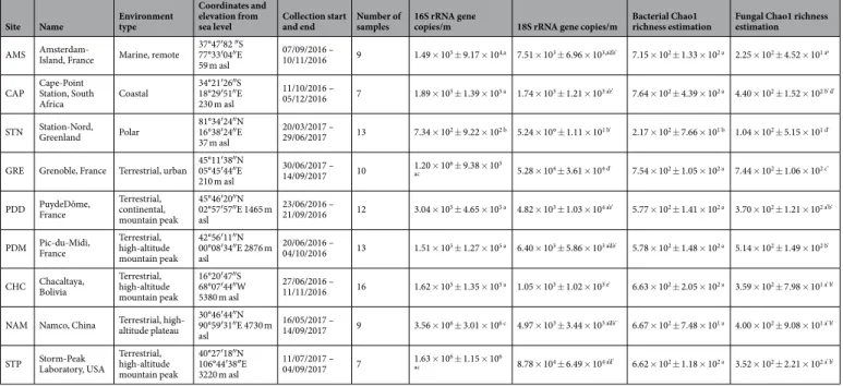
were the most abundant taxa of the dataset, although their relative abundances varied greatly based on sampling site. Bacterial and fungal concentration was the highest at the high-altitude and semi-arid plateau of Namco (China; 3.56 × 10⁶ ± 3.01 × 10⁶ cells/m3) and at the high-altitude and vegetated
mountain peak Storm-Peak (Colorado, USA; 8.78 × 10⁴ ± 6.49 × 10⁴ cells/m3), respectively. Surrounding
ecosystems, especially within a 50 km perimeter of our sampling stations, were the main contributors to the composition of airborne microbial communities. Temporal stability in the composition of airborne microbial communities was mainly explained by the diversity and evenness of the surrounding landscapes and the wind direction variability over time. Airborne microbial communities appear to be the result of large inputs from nearby sources with possible low and diluted inputs from distant sources.
Microbial transport in the atmosphere is critical for understanding the role microorganisms play in meteorology, atmospheric chemistry and public health. Recently, studies have shown that up to 106 microbial cells can be found
in one cubic meter of air1 and that they might be metabolically active2,3. Different processes, including
aerosolisa-tion and transport, might be important in selecting which microorganisms exist in the atmosphere. For example, specific bacterial taxa (e.g., Actinobacteria and some Gammaproteobacteria) have been proposed to be preferen-tially aerosolized from oceans4. Once aerosolized, microbial cells enter the planetary boundary layer, defined as
the air layer near the ground, directly influenced by the planetary surface, from which they might eventually be transported upwards by air currents into the free troposphere (air layer above the planetary boundary layer) or even higher into the stratosphere5–8. Microorganisms might undergo a selection process during their way up into
the troposphere and the stratosphere9. Studies from a limited number of sites have investigated possible processes
implicated in the observed microbial community distribution in the atmosphere, such as meteorology1,2,10–12,
seasons11,13–16, surface conditions12–14,16 and global air circulation11,17–20. Most research has described the airborne
microbial communities at one specific site per study. Airborne fungal communities (not only fungal spores) have frequently been overlooked, despite constituting a significant health concern for crops21,22 and in allergic
diseases23. A few have initiated the investigation of microbial geographic distribution by examining regional
and even continental patterns10,16,19, although in most cases at a few time points only. Some long-range transport
has been reported between regions separated by thousands of kilometers5,6. Several factors, such as the local
1Institut des Géosciences de l’Environnement, Univ Grenoble Alpes, CNRS, IRD, Grenoble INP, Grenoble, France. 2Environmental Microbial Genomics, Laboratoire Ampère, Ecole Centrale de Lyon, Université de Lyon, Ecully, France.
Correspondence and requests for materials should be addressed to R.T.-P. (email: [email protected])
Received: 19 June 2019 Accepted: 23 September 2019 Published online: 08 October 2019
Corrected: Author Correction
landscapes, local meteorological conditions, and inputs from long-range transport have all been cited as partially responsible for the composition of airborne microbial communities11,14,17,24–26, but their relative contribution
remains unclear. Probabilistically, proximity should have an effect, and therefore, local Earth sources of microor-ganisms should contribute significantly to atmospheric microbial communities especially in the planetary bound-ary layer. In addition, meteorological conditions (e.g., wind speed and direction) might lead to different temporal variability of airborne microbial communities by mediating the relative inputs of microbial populations from the different surrounding landscapes. Our goal was to evaluate the relative importance of environmental processes on the geographical and temporal variations in airborne microbial communities. This was carried out by following changes in community structure and abundance of both airborne bacteria and fungi as well as particulate matter chemistry and local meteorological characteristics over time at nine sites around the world.
Material and Methods
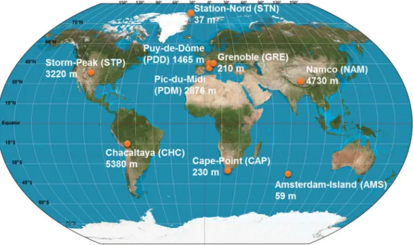
Air samples (seven to sixteen per site) were collected in 2016 and 2017 at nine sites from different latitudes (from the Arctic to the sub-Antarctica) and elevations from sea level (from 59 m to 5230 m; Fig. 1 and Supplementary Table S1). We collected particulate matter smaller than 10 µm (PM10) on pre-treated quartz fiber filters using high volume air samplers (TISCH, DIGITEL, home-made) equipped with a PM10 size-selective inlet. Quartz fiber fil-ters were heated to 500 °C for 8 hours to remove traces of organic carbon including DNA. All the material includ-ing the filter holders, aluminium foils and plastic bags in which the filters were transported were UV-sterilized as detailed in Dommergue et al., (2019)27. A series of field and transportation blank filters were done to monitor and
check the quality of the sampling protocol as presented in Dommergue et al., (2019)27.
The collection time per sample lasted one week. Depending on the site, the collected volumes ranged from 2000 m3 to 10000 m3 after standardization using SATP standards (Standard Ambient Pressure and
Temperature) (Supplementary Table S1). The environment type varied from marine (Amsterdam-Island) to coastal (Cape-Point), polar (Station-Nord) and terrestrial (Grenoble, Chacaltaya, Puy-de-Dôme, Pic-du-Midi, Storm-Peak and Namco) (Table 1). For mountain peaks, we sampled at night to minimize sampling in the plane-tary boundary layer (the filter was left in the sampler during day time). Detailed sampling protocols are presented in Dommergue et al., (2019)27. Elemental carbon (EC), organic carbon (OC), sugar anhydrides and alcohols
(levo-glucosan, mannosan, galactosan, inositol, glycerol, erythriol, xylitol, arabitol, sorbitol, mannitol, trehalose, rham-nose, glucose), major soluble anions (methylsulfonic acid [MSA], SO42−, NO3−, Cl−, oxalate) and cations (Na+,
NH4+, K+, Mg2+, Ca2+) were analyzed27.
At all sampling sites, meteorological parameters (i.e. wind speed and direction, temperature and relative humidity) were collected every hour. Meteorological data were used to produce wind roses using the openair R package28. For each sample, backward trajectories of the air masses were calculated over 3 days (maximum height
from sea level: 1 km) using HYSPLIT29 and plotted on geographical maps using the openair R package.
We extracted DNA from 3 circular pieces (punches) from the quartz fiber filters (diameter of one punch: 38 mm) using the DNeasy PowerWater kit with the following modifications as detailed in Dommergue et al.,
(2019)27. During the cell lysis, we heated at 65°c the PowerBead tube containing the 3 punches and the pre-heated
lysis solution during one hour after a 10-min vortex treatment at maximum speed. We then centrifuged the mixture at 1000 rcf during 4 min to separate the filter debris from the lysate using a syringe. From this step, we continued the extraction following the DNeasy PowerWater protocol. DNA concentration was measured using the High Sensitive Qubit Fluorometric Quantification (Thermo Fisher Scientific) then DNA was stored at −20 °C.
Real-time qPCR analyses on the 16S rRNA (data previously published in Dommergue et al., (2019)27) and 18S
rRNA genes were carried out (regions, primers30,31 and protocols in Supplementary Information) to
approxi-mate the concentration of bacterial and fungal cells per cubic meter of air. Although bacteria and fungi might have more than one copy of 16S rRNA and 18S rRNA gene per genome, respectively, attempts to correct for metagenomics datasets are unproductive32. Microbial community structure was obtained using MiSeq Illumina
amplicon sequencing of the bacterial V3-V4 region of the 16S rRNA gene and the fungal ITS2 region. The library preparation protocol, read quality filtering and taxonomic annotation of every sequence using RDP Classifier33
are detailed in Supplementary Information. RDP classifier was used in part to avoid errors due to sequence clus-tering. The raw read number per sample and the percentage of sequences annotated using RDP Classifier for both the 16S rRNA gene and ITS sequencings are presented in Supplementary Table S1.
All graphical and multivariate statistical analyses were carried out in the R environment, using the vegan34,
pvclust35, ade436 and Hmisc37 R packages. The raw abundances of the bacterial genera or fungal species were
transformed in relative abundances to counter the heterogeneity in the number of sequences per sample and then standardized using Hellinger’s transformation. Chao1 estimations of the richness for both bacterial and fungal communities were calculated and averaged for each site. MODIS (Moderate resolution imaging spectroradiom-eter) land cover approach (5′ × 5′ resolution)38,39 was used to quantify landscapes in a diameter range of the
sam-pling sites (50, 100 and 300 km). The perimeter of 50 km was chosen because the landscapes were best correlated to airborne microbial community structures. The different MODIS land covers are described in Supplementary Table S2. We weighted these relative surfaces by their associated bacterial cell concentration reported by Burrows
et al., (2009)40,41 (Supplementary Table S3) to predict the relative contribution of each landscape to the aerial
emission of bacterial cells.
Hierarchical clustering analyses (average method) were carried out on either the Bray-Curtis dissimilarity matrix (bacterial and fungal community structure) or the Euclidean distance matrix (PM10 chemistry, land-scapes and the relative contributions of the landland-scapes). A Mantel test was used to evaluate the similarities in the distribution of the samples in the different data sets. Distance-based redundancy analyses (RDA) were car-ried out to evaluate the part of the variance between the samples based on the microbial community structure explained by chemistry. Prior to the cluster analysis based of the chemical dataset, chemical concentrations were log10-transformed to approach a Gaussian distribution. SIMPER analysis was used to identify the major bacterial or fungal contributors to the difference between the detected groups.
Spearman correlations were calculated to test the correlation between microbial abundance and richness and quantitative environmental factors like chemical concentrations or meteorological parameters. ANOVAs were used to test the influence of qualitative factors such as localization on both bacterial and fungal abundance and richness and TukeyHSD tests to identify which group had a significantly different mean. To compare the temporal variability in microbial communities at each site, we interpreted both the Bray-Curtis dissimilarity value averaged per site and the associated standard deviation. We calculated a new statistic, i.e. a similarity index, as follows. We averaged the values of dissimilarity obtained from the Bray-Curtis matrix for each pair of samples from the same Site Name Environment type
Coordinates and elevation from
sea level Collection start and end Number of samples 16S rRNA gene copies/m 18S rRNA gene copies/m Bacterial Chao1 richness estimation Fungal Chao1 richness estimation
AMS Amsterdam-Island, France Marine, remote 37°47′82 ″S 77°33′04″E 59 m asl
07/09/2016 –
10/11/2016 9 1.49 × 10⁵ ± 9.17 × 10⁴,a 7.51 × 10³ ± 6.96 × 10³,a’d’e’ 7.15 × 10² ± 1.33 × 10² a 2.25 × 10² ± 4.52 × 101 a’ CAP Cape-Point Station, South
Africa Coastal 34°21′26″S 18°29′51″E 230 m asl 11/10/2016 – 05/12/2016 7 1.89 × 10⁵ ± 1.39 × 10⁵ a 1.74 × 10³ ± 1.21 × 10³ a’e’ 7.64 × 10² ± 4.39 × 10² a 4.40 × 10² ± 1.52 × 10² b’ d’ STN Station-Nord, Greenland Polar 81°34′24″N 16°38′24″E
37 m asl
20/03/2017 –
29/06/2017 13 7.34 × 10² ± 9.22 × 10² b 5.24 × 10° ± 1.11 × 101 b’ 2.17 × 10² ± 7.66 × 101 b 1.04 × 10² ± 5.15 × 101 d’ GRE Grenoble, France Terrestrial, urban 45°11′38″N 05°45′44″E
210 m asl
30/06/2017 –
14/09/2017 10 1.20 × 10
6 ± 9.38 × 10⁵
ac 5.28 × 10⁴ ± 3.61 × 10⁴ d’ 7.54 × 10² ± 1.05 × 10² a 7.44 × 10² ± 1.06 × 10² c’
PDD PuydeDôme, France Terrestrial, continental, mountain peak 45°46′20″N 02°57′57″E 1465 m asl 23/06/2016 – 21/09/2016 12 3.04 × 10⁵ ± 4.65 × 10⁵ a 4.82 × 10³ ± 1.03 × 10⁴ a’e’ 5.77 × 10² ± 1.41 × 10² a 3.70 × 10² ± 1.21 × 10² a’b’ PDM Pic-du-Midi, France Terrestrial, high-altitude
mountain peak 42°56′11″N 00°08′34″E 2876 m asl 20/06/2016 – 04/10/2016 13 1.51 × 10⁵ ± 1.27 × 10⁵ a 6.40 × 10³ ± 5.86 × 10³ a’d’e’ 5.78 × 10² ± 1.48 × 10² a 5.14 × 10² ± 1.49 × 10² b’ CHC Chacaltaya, Bolivia Terrestrial, high-altitude
mountain peak 16°20′47″S 68°07′44″W 5380 m asl 27/06/2016 – 11/11/2016 16 1.62 × 10⁵ ± 1.35 × 10⁵ a 1.05 × 10³ ± 1.02 × 10³ e’ 6.63 × 10² ± 2.05 × 10² a 3.59 × 10² ± 7.98 × 101 a’ b’ NAM Namco, China Terrestrial, high-altitude plateau 30°46′44″N 90°59′31″E 4730 m
asl
16/05/2017 –
14/09/2017 9 3.56 × 10⁶ ± 3.01 × 10⁶ c 4.97 × 10³ ± 3.44 × 10³ a’d’e’ 6.67 × 10² ± 7.48 × 101 a 4.00 × 10² ± 9.08 × 101 a’ b’ STP Storm-Peak Laboratory, USA Terrestrial, high-altitude
mountain peak 40°27′18″N 106°44′38″E 3220 m asl 11/07/2017 – 04/09/2017 7 1.63 × 10 6 ± 1.15 × 10⁶ ac 8.78 × 10⁴ ± 6.49 × 10⁴ a’d’ 6.62 × 10² ± 1.18 × 10² a 3.52 × 10² ± 2.21 × 10² a’ b’
Table 1. Summary of bacterial and fungal abundances and bacterial (genus level) and fungal (species level)
Chao1 richness estimations averaged per site and associated to a standard deviation. Reference letters indicate the group membership based on Tukey’s HSD post hoc tests. The environment type, coordinates, elevation from sea level, collection start and end per site and the number of samples collected per site are shown. The 16S rRNA gene qPCR data was previously published in Dommergue et al., (2019)27.
site. Then we subtracted these values from 1 to get similarity values and finally we divided the similarity values by the standard deviation −
(
Bray Curtis dissimilarity value averaged per site)
Bray Curtis standard deviation
1 . The higher is the similarity in microbial
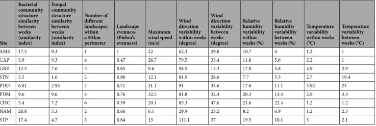
com-munity structure between the samples, the higher is the similarity index. A multiple linear regression model was used to test the influence of wind and surrounding landscape characteristics (number of different landscapes and landscape evenness) of the sites on the temporal variability of both the fungal and bacterial community structure (evaluated by the similarity index). Pielou’s evenness was used to determine how similar the different relative surfaces of each landscape surrounding the sites were. The temporal variability of meteorological parameters was calculated both within weekly samples (average variance of hourly data for one week) and between weekly sam-ples of the same site (standard deviation of the above average variance over weeks).
Results
Geographical distribution of airborne microbial communities.
Airborne microbial concentrations varied between 9.2 × 101 to 1.3 × 10⁸ cells per cubic meter of air for bacteria and from not detectable (< 2 × 10°)to 1.9 × 10⁵ cells per cubic meter of air for fungi. A high correlation was observed between the bacterial and the
fungal concentrations from all the sites and all sampling times (N = 95, R = 0.85, P = 2.2 × 10⁻¹⁶). The average
bacterial and fungal concentrations per site varied from 7.3 × 10² to 3.6 × 10⁶ and from 5.2 × 10° to 8.8 × 10⁴ cells
per cubic meter of air, respectively, and were different between the sites (P = 2.2 × 10⁻¹¹ and P = 5.7 × 10⁻¹⁵ for
bacteria and fungi, respectively; Table 1). The polar site Station-Nord and the high altitude plateau site of Namco had the lowest and highest average bacterial concentration, respectively. The highest average fungal concentration was observed in atmospheric samples from the urban site of Grenoble and the mountain site of Storm-Peak, while the lowest was from Station-Nord (Table 1).
The most abundant bacterial genera overall for all the samples were Bacillus (8.23%), Sphingomonas (5.62%),
Hymenobacter (4.32%), Romboutsia (2.77%), Methylobacterium (2.63%), and Clostridium (2.18%) (a list of the
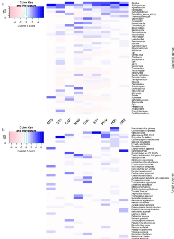
highest 50 genera is shown in Supplementary Table S4), although their relative contribution to each site varied. A heatmap of the relative abundances of the fifty most abundant bacterial genera in each site is represented in Fig. 2. For example, Bacillus averaged 15.63% relative abundance in Puy-de-Dôme samples, but only 0.03% in the marine Amsterdam-Island samples. Average bacterial Chao1 richness estimations varied between 577 + − 141 (Puy-de-Dôme) and 217 + − 76 (Station-Nord). They did not differ significantly (P > 0.05) between sites with the exception of Station-Nord which showed the lowest Chao1 value (P = 4.9 × 10⁻¹¹) (Table 1). The most abundant
fungal species in the whole dataset were Pseudotaeniolina globosa (5.44%), Cladophialophora proteae (3.67%),
Ustilago bullata (3.22%), Alternaria sp (2.60%), and Botryotinia fuckeliana (Botrytis cinerea) (2.47%) (a list of the
highest 50 species is shown in Supplementary Table S5), although their relative contribution to each site varied. A heatmap of the relative abundances of the fifty most abundant fungal species in each site is represented in Fig. 2. For example, Pseudotaeniolina globosa averaged 11.47% relative abundance in Puy-de-Dôme samples, but less than 0.01% in Station-Nord and Storm-Peak samples. Average fungal Chao1 richness estimations were different between the sites (P = 9.5 × 10⁻¹⁴) with the highest value from Grenoble (742 +/− 106) and lowest values from
Cape-Point (440 +/−152), Amsterdam-Island (225 +/− 45) and Station-Nord (104 +/− 51). The bacterial and fungal Chao1 richness estimations correlated with the bacterial and fungal concentrations, respectively (N = 81,
R = 0.61, P = 1.0 × 10⁻⁹ and N = 79, R = 0.58, P = 2.0 × 10⁻⁸, respectively).
The different temporal samples grouped mainly by their site of origin using the hierarchical cluster analyses based on both their bacterial and fungal community structure (Fig. 3; for an expanded view see Supplementary Fig. S1) and using the bacterial and fungal community profiles averaged over the multiple samples per site (Fig. 4
and Supplementary Fig. S2). The sites grouped into three distinct clusters on both the bacterial and fungal-based trees: one cluster included the marine site Amsterdam-Island, the second the polar site Station-Nord and the third one included all the terrestrial and non-polar sites including the coastal site Cape-Point (Fig. 4 and Supplementary Fig. S2). The different sites or groups of sites were characterized by bacterial genera and fungal species known to be associated to the environment type of the site in most cases (Supplementary Table S6). The temporal var-iability of the composition of the bacterial and fungal communities at each site was different between the sites (P < 2 × 10⁻¹⁶ for both bacterial and fungal communities; Table 2). Temporal variations in the bacterial
commu-nity structure were not correlated to the variations in the fungal commucommu-nity structure (R = 0.13, P = 0.74). The highest temporal variability of the composition of the bacterial communities was observed in Cape-Point (sim-ilarity index of 3.9), Chacaltaya (5.4) and Station-Nord (5.5), while the lowest temporal variability was observed in Amsterdam-Island (17.5), Storm-Peak (17.4) and Namco (20.8). The highest temporal variability of the com-position of the fungal communities was observed in Station-Nord (similarity index of 1.6), Puy-de-Dôme (2.95) and Storm-Peak (4.7), while the lowest temporal variability was observed in Amsterdam-Island (9.3), Cape-Point (9.3) and Pic-du-Midi (9.6; Table 2). We observed eight “outlier” samples (i.e. samples which did not group with the other samples of their respective site) out of eighty-two samples using the hierarchical cluster analysis based on the bacterial community structure of the individual samples (Fig. 3). Only one outlier was observed using the hierarchical cluster analysis based on the fungal community structure (Fig. 3).
Potential factors driving chemistry and microbiology.
Samples from the same site tended to group together based on the PM10 chemistry using hierarchical cluster analysis (Supplementary Fig. S3). Therefore, we calculated the average chemical profile for each site and redid the cluster analysis (Fig. 4). The sites were separated into three main clusters using a hierarchical cluster analysis based on the average chemical profiles (Fig. 4): the first cluster (Amsterdam-Island, Cape-Point) was characterized by high relative concentrations of sea salts (Cl, Na), the second (Puy-de-Dôme, Grenoble, Pic-du-Midi, Chacaltaya, Namco, Storm-Peak) by higher concentra-tions of organic carbon, polyols and sugars, and the third (Station-Nord) by very low relative concentraconcentra-tions of polyols and sugars and lower relative concentrations of sea salts compared to the first cluster (SupplementaryTable S7). The PM10 chemistry was correlated to the bacterial and fungal community structure averaged over the multiple samples per site (Mantel test R = 0.79 P = 0.007 and R = 0.68 and P = 0.02, respectively) (see RDA figures in Supplementary Fig. S4). The differences between the marine site (Amsterdam-Island), coastal site (Cape-Point), polar site (Station-Nord) and terrestrial sites in terms of PM10 chemistry and microbial com-munities might create this correlation. Thus, we looked at the correlation using only the terrestrial sites and the correlation between the PM10 chemistry and the bacterial and fungal community structure was weaker (R = 0.16,
P = 0.33 and R = 0.51, P = 0.03 for bacterial and fungal community structure, respectively).
Figure 2. Heatmaps of the relative abundances (the relative abundances are centered and scaled) of the fifty
most abundant bacterial genera (a) and fungal species (b) in the dataset. The fifty bacterial genera and fungal species are in order of decreasing relative abundance from top to bottom.
The different landscapes (e.g., forest, cropland, ocean, etc.) surrounding the sites were identified using the MODIS land cover approach (Fig. 4). We weighted the relative surface of the different landscapes by their asso-ciated bacterial cell concentration reported by Burrows et al., (2009)40,41 to predict the relative contribution of
each landscape to the aerial emission of bacterial cells at each site (Fig. 4). Terrestrial sites grouped together based on the high contribution of their terrestrial landscape to the aerial emission of bacterial cells. The average PM10 chemical profile for the different sites was only correlated to the relative surfaces of the different land-scapes when considering all the sites (R = 0.77, P = 0.001), but not when considering only the terrestrial sites (R = 0.32, P = 0.1). Both the bacterial and fungal communities were correlated to the landscapes over all the sites (R = 0.80, P = 0.001; R = 0.64, P = 0.003, respectively). However, unlike the chemistry, the bacterial community structure averaged over the multiple samples was correlated to the relative surfaces of the different landscapes for the terrestrial sites (R = 0.65, P = 0.004). The same was observed for the fungal community structure averaged over the multiple temporal samples which was also correlated to the landscapes of the terrestrial sites (R = 0.47,
P = 0.05). Although the bacterial community distribution was correlated to the fungal community distribution
(R = 0.82, P = 0.006), some differences were observed. The mountain sites (Namco, Chacaltaya, Storm-Peak and Pic-du-Midi) grouped together in the cluster analysis based on their bacterial community structure, while the sites characterized by croplands as one of their surrounding landscapes (Grenoble, Pic-du-Midi, Puy-de-Dôme and Cape-Point) grouped together in the cluster analysis based on the fungal community diversity (Fig. 4 and Supplementary Fig. S2 for the cluster analysis based on the bacterial and fungal diversity, respectively).
Meteorological characteristics (wind speed and hourly variations in wind direction, relative humidity, and temperature over one week and between weeks) were different between the sites (Table 2). Puy-de-Dôme, Pic-du-Midi and Cape-Point showed episodes of high wind speeds (between 26 and 32 m/s), while the wind speed did not reach 10 m/s in Grenoble and Namco. The wind direction varied within the weeks of sampling and also between the multiple weekly samples per site, and these variations were not necessarily correlated. For example, the wind direction in Grenoble varied continually within the weeks (mean variability within weeks: 94.5°), and this variability did not change much between the weeks (mean variability between weeks: 34.6°). The wind direction in Chacaltaya changed less within the weeks (35.3°) than between the weeks (47.6°). The differ-ent temporal variability of both the wind speed and direction led to differdiffer-ent wind roses and backward air mass
Figure 3. Hierarchical cluster analysis (average method) of the Bray-Curtis dissimilarity matrices based on
the (a) V3-V4 region of the 16S rRNA gene (genus level) and (b) ITS region (species level). Colored rectangles correspond to samples of the same site or group of sites stated beside the rectangles. Outlier samples (samples which were outside their expected group) are circled in grey. Samples are named as follows: site_date.of. sampling.
trajectories with different directions and lengths at each site (Supplementary Figs S5,S6). The relative humidity and temperature also showed a different temporal (within and between weeks) variability depending on the site (Table 2). Multiple linear regressions between the level of temporal variability of both the bacterial and fungal community structures at each site and the meteorological and surrounding landscape characteristics (number of different landscapes and landscape evenness) were calculated. For the variation of bacterial composition over time, the regression included the wind direction variability within and between weeks, the temperature variabil-ity between weeks and the landscape evenness (R squared = 0.93, adjusted R squared = 0.82, P = 0.06). For the variation of fungal composition over time, the wind speed and temperature variability between weeks were the best parameters (R squared = 0.87, adjusted R squared = 0.83, P = 0.002) (Supplementary Table S8 and Fig. S7).
Discussion
Airborne particulate matter (PM) is thought to undergo both short and long-range transport depending mainly on particle size42–44. Airborne microbial cells might exist both as free cells and in association to PM in the
atmos-phere45–47. This means that the sources, transport duration and deposition processes could be different between
PM and microbial cells, especially if their size distribution is different. Furthermore, the potential transformation processes that they might undergo during atmospheric transport are likely to be different. While photochemistry and gas condensation will change the chemical composition and size distribution of PM48, selective processes
associated mainly to UV radiation, desiccation and cold temperatures could lead to the death, sporulation and genetic mutations of microbial cells, although the occurrence of these processes in the atmosphere have been rarely explored17,49. Thus, a correlation between airborne microbial community structure and the chemical
com-position of PM is unlikely due to their expected differential fate during transportation in the atmosphere. So while
Figure 4. Distribution of the sites based on the different data sets (bacterial community structure, PM10
chemistry, landscapes, relative contributions of the different landscapes in the aerial emission of bacterial cells). (a) Hierarchical cluster analysis (average method) on the Euclidean distance matrix based on the PM10 chemistry. (b) Relative surfaces of the different landscapes surrounding the sites (perimeter of 50 km) based on the MODIS land cover approach. (c) Relative contributions of the different landscapes in the aerial emission of bacterial cells (based on the study of Burrows et al., (2009)40). (d) Hierarchical cluster analysis (average method)
on the Bray-Curtis dissimilarity matrix based on the bacterial community structure (genus level). Bootstrap values in percentage are indicated over each node on both cluster analyses.
PM10 chemistry correlated to both the bacterial (R = 0.79, P = 0.007) and fungal (R = 0.68, P = 0.02) community structures over all the sites, the correlation was considerably less for the terrestrial sites for bacteria (R = 0.16,
P = 0.33) and fungi (R = 0.51, P = 0.03). The strong correlation observed when considering all the sites might be
more indicative of strong differences between the different ecosystems (marine, polar, coastal and terrestrial) in terms of chemistry and microbial communities than a similar behavior and/or driving processes of the PM10 and microbial cell distribution.
This weak correlation between PM10 chemistry and airborne bacterial communities over the terrestrial sites has been observed previously1,18, but certain chemicals might affect specific microbial populations without
influ-encing the overall correlation. For example, methylsulfonic acid (MSA) was correlated to the genus Acholeplasma (R = 0.88, P = 1.7 × 10⁻³). Certain polyol concentrations were correlated to the relative abundance of specific
fungi (e.g., mannitol-arabitol and the species Zalerion arboricola R = 0.85, P = 3.9 × 10⁻³). Polyols can be major
components of fungal biomass and have been proposed as a suitable marker for fungal spores50. We currently
do not know whether these chemistry-microbial genera/species correlations are due to similar sources for both PM10 and microorganisms or that the chemistry is selecting for these microorganisms during atmospheric transportation.
The similarity of the sites based on the PM10 chemistry globally matched the similarity of the sites based on the characteristics of the landscapes surrounding the sites (Fig. 4). However, since the correlation between the chemistry and the characteristics of the surrounding area was not very high when considering only the terrestrial sites (R = 0.32, P = 0.1), distant sources and/or photochemical transformations (formation of secondary aerosols) likely also contribute to the PM10 chemistry distribution. A strong correlation was observed between both air-borne bacterial (R = 0.80, P = 0.001 with all the sites; R = 0.65, P = 0.004 with only the terrestrial sites) and fungal community structure (R = 0.64, P = 0.003 with all the sites; R = 0.47, P = 0.05 with only the terrestrial sites) and the landscapes (Fig. 4 and Supplementary Fig. S2). This correlation illustrates the important contribution of the local landscapes to the geographical distribution of airborne microorganisms. The landscapes with the most impact on the distribution of atmospheric microorganisms between the sites were ice, water, forest, grassland and cropland. These landscapes might emit distinct communities as compared to the others such as urban landscapes which did not seem to significantly contribute to the observed geographical microbial distribution of the sites. Regional environmental factors, and specifically, a combination of climate and soil characteristics (but no effect from urbanization) have been reported to correlate to the geographical distribution of dust-associated microbial communities10. Reports of other smaller-scale studies2,13,16,18 suggested a strong influence of the local sources
in the spatial distribution of airborne microbial communities. Airborne microbial community structure at the coastal site Cape-Point was more similar to that for terrestrial sites than those from marine or polar sites. This might reflect that terrestrial landscapes contribute more biomass to airborne microbial communities than oceanic landscapes, as was proposed by Burrows et al., (2009)40,41.
Our airborne bacterial concentrations were mainly correlated to the surrounding landscape. We observed the highest atmospheric bacterial concentrations at the grassland sites (Namco, Storm-Peak) and urban and cropland sites (Grenoble, Puy-de-Dôme), followed by the coastal site (Cape-Point), marine site (Amsterdam-Island) and polar site (Station-Nord). We did not observe the highest average concentration of bacteria at the most urban site (Grenoble) as expected based on the study of Burrows et al., (2009)40,41, although Grenoble might not be as
indus-trial as others reported in the literature1,11. Instead, the highest average concentration of bacteria was observed at
Namco, which is a remote high-altitude and semi-arid grassland site (grassland covers >80% of the surrounding landscape over 50 km of diameter). Pic-du-Midi (cropland/vegetation) and Chacaltaya (grassland), which are two high-altitude mountain peaks, had relatively low average bacterial concentrations that were comparable to
Site Bacterial community structure similarity between weeks (similarity index) Fungal community structure similarity between weeks (similarity index) Number of different landscapes within a 50 km perimeter Landscape evenness (Pielou’s evenness) Maximum wind speed (m/s) Wind direction variability within weeks (degree) Wind direction variability between weeks (degree) Relative humidity variability within weeks (%) Relative humidity variability between weeks (%) Temperature variability within weeks (°C) Temperature variability between weeks (°C) AMS 17.5 9.3 1 1 22 62.3 29.8 10.7 4 1.2 1 CAP 3.9 9.3 4 0.47 26.7 79.5 33.4 11.8 5.6 2.2 1 GRE 12.5 7.6 5 0.65 9.6 94.5 15.3 17.8 5.8 4.9 2.9 STN 5.5 1.6 2 0.80 12.1 81.9 28.6 7.7 5.3 2.7 19.4 PDD 6.81 2.95 4 0,71 31.1 91 34.6 17.6 11.1 3.92 23 PDM 9.6 9.6 4 0.76 32.5 81.8 32.4 20.3 13.4 2.9 3.3 CHC 5.4 7.2 6 0.59 20.1 85.3 47.6 21.6 22.4 1.2 1.2 NAM 20.8 5.3 2 0.66 6.1 29.9 23.2 8.2 6.9 1.2 2.3 STP 17.4 4.7 3 0.84 13 111.1 37 19.5 10.1 3 2.1
Table 2. Temporal variability of the microbial community structure and meteorological conditions at each site.
The similarity index was calculated as following: (1 – Bray-Curtis dissimilarity value averaged per site)/standard deviation. The maximum wind speed (m/s) per site, the variability of the wind direction (degree), relative humidity (%) and temperature (°C) within a week and between the weeks, the number of different landscapes within a perimeter of 50 km and the landscape evenness are shown.
the average bacterial concentration of the coastal site Cape-Point. The elevation and steep slopes of Pic-du-Midi and Chacaltaya could explain the relatively low airborne bacterial concentrations, since they might limit upward migration of aerosolized bacteria from land surfaces to peaks. Another explanation could be that Chacaltaya and Pic-du-Midi aerosols were sampled mainly from the free-troposphere that has fewer microorganisms than the planetary boundary layer. At the Namco site, the calm meteorological conditions (low wind speed, low relative humidity and a low precipitation rate), in association with the high dust content of the surrounding landscape could explain its high bacterial concentrations. The effect of meteorological conditions on airborne microbial concentrations have been investigated previously51–53, but the wind speed, for example, could lead to either an
increase or a decrease in the bacterial concentration depending on its direction, speed and site characteristics. We hypothesized that meteorological conditions could have an influence on the temporal variation of air-borne microbial community structure by affecting the relative inputs of different microbial populations from different surrounding landscapes. Our data showed that the temporal variability of microbial community struc-ture was significantly different between the sites and could be correlated (R > 0.80) with wind condition varia-bility, temperature variability and/or landscape characteristics (number of different landscapes and landscape evenness). Wind conditions and temperature are both known to affect the aerosolization process54,55. The wind
speed was an important factor explaining fungal variability as different wind speeds might lift up different fungal spore sizes and weights56,57. The characteristics of the surrounding landscape (number of different landscapes
and landscape evenness) were also important factors determining the temporal variability of airborne microbial communities. Namco and Amsterdam-Island had relatively low temporal variability of airborne bacterial com-munity structure in concordance with their relatively monospecific landscapes, grassland and oceanic, respec-tively. Although Amsterdam-Island site is characterized by high wind speed, the presence of an oceanic surface over a large perimeter around the site imposed a predominance of homogeneous atmospheric microbial com-munities. Consequently, wind speed and direction could be of importance when the surrounding landscape is diverse. Although Grenoble has five different surrounding landscapes, the low wind speed (<9.6 m/s) in Grenoble would lead to a relatively low temporal variability of the airborne bacterial community structure. Conversely, the association of different surrounding landscapes and a medium (between 12 m/s and 13 m/s) or high wind speed (>22 m/s), as found at the other sites would increase the variability of the composition of bacterial communities over time as a function of the wind speed, wind direction variability and the number of different landscapes. We think that the changes in the composition of airborne bacterial communities might be due to the combined effect of changes in landscapes and local meteorological conditions. Changes in seasons will likely affect landscapes and meteorological conditions and, therefore, influence microbial community composition13–16,18,58.
conclusion
This is the first worldwide-scale study investigating airborne microbial communities at diverse sites in terms of latitudinal position, type of ecosystem, surrounding landscapes and local meteorological conditions. We also investigated the atmospheric particulate matter, surrounding landscapes via the MODIS land cover approach, and local meteorology to assess their role in defining the atmospheric microbial communities. We observed that air-borne microbial communities were correlated to the surrounding landscapes, although some (minor fraction) of the microbial cells might travel over long distances. While two sites sharing similar surrounding landscapes will likely get a similar airborne microbial profile, different local meteorological conditions will control the stability of this microbial profile through time. In the context of global warming and land use changes atmospheric microbial (including viruses) communities should be continually monitored around our planet.
Data Availability
Sequences reported in this paper have been deposited in ftp://ftp-adn.ec-lyon.fr/aerobiology_amplicon_IN-HALE/. A file has been attached explaining the correspondence between file names and samples.
References
1. Zhen, Q. et al. Meteorological factors had more impact on airborne bacterial communities than air pollutants. Sci. Total Environ.
601–602, 703–712 (2017).
2. Šantl-Temkiv, T., Gosewinkel, U., Starnawski, P., Lever, M. & Finster, K. Aeolian dispersal of bacteria in southwest Greenland: their sources, abundance, diversity and physiological states. FEMS Microbiol. Ecol 94 (2018).
3. Klein, A. M., Bohannan, B. J. M., Jaffe, D. A., Levin, D. A. & Green, J. L. Molecular Evidence for Metabolically Active Bacteria in the Atmosphere. Front. Microbiol. 7 (2016).
4. Michaud, J. M. et al. Taxon-specific aerosolization of bacteria and viruses in an experimental ocean-atmosphere mesocosm. Nat
Commun 9, 2017 (2018).
5. Griffin, D. W., Gonzalez‐Martin, C., Hoose, C. & Smith, D. J. Global-Scale Atmospheric Dispersion of Microorganisms. in Microbiology of Aerosols 155–194, https://doi.org/10.1002/9781119132318.ch2c (John Wiley & Sons, Ltd, 2017).
6. Smith, D. J., Griffin, D. W. & Jaffe, D. A. The high life: Transport of microbes in the atmosphere. Eos Trans. AGU 92, 249–250 (2011). 7. Smith, D. J. et al. Airborne Bacteria in Earth’s Lower Stratosphere Resemble Taxa Detected in the Troposphere: Results From a New
NASA Aircraft Bioaerosol Collector (ABC). Front Microbiol 9, 1752 (2018).
8. Maki, T. et al. Assessment of composition and origin of airborne bacteria in the free troposphere over Japan. Atmospheric
Environment 74, 73–82 (2013).
9. Els, N., Baumann-Stanzer, K., Larose, C., Vogel, T. M. & Sattler, B. Beyond the planetary boundary layer: Bacterial and fungal vertical biogeography at Mount Sonnblick, Austria. Geo: Geography and Environment 6, e00069 (2019).
10. Barberán, A. et al. Continental-scale distributions of dust-associated bacteria and fungi. Proc. Natl. Acad. Sci. USA 112, 5756–5761 (2015).
11. Innocente, E. et al. Influence of seasonality, air mass origin and particulate matter chemical composition on airborne bacterial community structure in the Po Valley, Italy. Sci. Total Environ. 593–594, 677–687 (2017).
12. Uetake, J. et al. Seasonal changes of airborne bacterial communities over Tokyo and influence of local meteorology. bioRxiv 542001,
https://doi.org/10.1101/542001 (2019).
13. Bowers, R. M., McLetchie, S., Knight, R. & Fierer, N. Spatial variability in airborne bacterial communities across land-use types and their relationship to the bacterial communities of potential source environments. ISME J 5, 601–612 (2011).
14. Bowers, R. M., McCubbin, I. B., Hallar, A. G. & Fierer, N. Seasonal variability in airborne bacterial communities at a high-elevation site. Atmospheric Environment 50, 41–49 (2012).
15. Bowers, R. M. et al. Seasonal variability in bacterial and fungal diversity of the near-surface atmosphere. Environ. Sci. Technol. 47, 12097–12106 (2013).
16. Mhuireach, G. Á., Betancourt-Román, C. M., Green, J. L. & Johnson, B. R. Spatiotemporal Controls on the Urban Aerobiome. Front.
Ecol. Evol. 7 (2019).
17. Cáliz, J., Triadó-Margarit, X., Camarero, L. & Casamayor, E. O. A long-term survey unveils strong seasonal patterns in the airborne microbiome coupled to general and regional atmospheric circulations. Proc. Natl. Acad. Sci. USA 115, 12229–12234 (2018). 18. Gandolfi, I. et al. Spatio-temporal variability of airborne bacterial communities and their correlation with particulate matter
chemical composition across two urban areas. Appl. Microbiol. Biotechnol. 99, 4867–4877 (2015).
19. Fröhlich-Nowoisky, J. et al. Biogeography in the air: fungal diversity over land and oceans. Biogeosciences 9, 1125–1136 (2012). 20. Mayol, E. et al. Long-range transport of airborne microbes over the global tropical and subtropical ocean. Nature Communications
8, 201 (2017).
21. Fisher, M. C. et al. Emerging fungal threats to animal, plant and ecosystem health. Nature 484, 186–194 (2012).
22. Brown, J. K. M. & Hovmøller, M. S. Aerial dispersal of pathogens on the global and continental scales and its impact on plant disease.
Science 297, 537–541 (2002).
23. Żukiewicz-Sobczak, W. A. The role of fungi in allergic diseases. Postepy Dermatol Alergol 30, 42–45 (2013).
24. Vaïtilingom, M. et al. Long-term features of cloud microbiology at the puy de Dôme (France). Atmospheric Environment 56, 88–100 (2012).
25. Yamamoto, N. et al. Particle-size distributions and seasonal diversity of allergenic and pathogenic fungi in outdoor air. ISME J 6, 1801–1811 (2012).
26. Fierer, N. et al. Short-Term Temporal Variability in Airborne Bacterial and Fungal Populations. Appl Environ Microbiol 74, 200–207 (2008).
27. Dommergue, A. et al. Methods to investigate the global atmospheric microbiome. Front. Microbiol. 10 (2019). 28. Carslaw, D. Tools for the Analysis of Air Pollution Data (2019).
29. Draxler, R. R. & Hess, G. D. An Overview of the HYSPLIT_4 Modelling System for Trajectories, Dispersion, and Deposition. Aust.
Met. Mag. 47, 295–305 (1998).
30. Fierer, N., Jackson, J. A., Vilgalys, R. & Jackson, R. B. Assessment of Soil Microbial Community Structure by Use of Taxon-Specific Quantitative PCR Assays. Appl. Environ. Microbiol. 71, 4117–4120 (2005).
31. Chemidlin Prévost-Bouré, N. et al. Validation and application of a PCR primer set to quantify fungal communities in the soil environment by real-time quantitative PCR. PLoS ONE 6, e24166 (2011).
32. Louca, S., Doebeli, M. & Parfrey, L. W. Correcting for 16S rRNA gene copy numbers in microbiome surveys remains an unsolved problem. Microbiome 6 (2018).
33. Wang, Q., Garrity, G. M., Tiedje, J. M. & Cole, J. R. Naive Bayesian Classifier for Rapid Assignment of rRNA Sequences into the New Bacterial Taxonomy. Applied and Environmental Microbiology 73, 5261–5267 (2007).
34. Oksanen, J. et al. Community Ecology Package (2019).
35. Suzuki, R. & Shimodaira, H. Hierarchical Clustering with P-Values via Multiscale BootstrapResamplin. (2015).
36. Dray, S., Dufour, A.-B. & Thioulouse, J. Analysis of Ecological Data: Exploratory and Euclidean Methodsin Environmental Science (2018).
37. Harrell, F. E. & Dupont, C. Harrell Miscellaneous - Package ‘Hmisc’. (2019).
38. Shannan, S., Collins, K. & Emanuel, W. R. Global mosaics of the standard MODIS land cover type data. (2014).
39. Friedl, M. A. et al. Global land cover mapping from MODIS: algorithms and early results. Remote Sensing of Environment 83, 287–302 (2002).
40. Burrows, S. M., Elbert, W., Lawrence, M. G. & Pöschl, U. Bacteria in the global atmosphere – Part 1: Review and synthesis of literature data for different ecosystems. Atmos. Chem. Phys. 9, 9263–9280 (2009).
41. Burrows, S. M. et al. Bacteria in the global atmosphere – Part 2: Modeling of emissions and transport between different ecosystems.
Atmospheric Chemistry and Physics 9, 9281–9297 (2009).
42. Alebic-Juretic, A. & Mifka, B. Secondary Sulfur and Nitrogen Species in PM10 from the Rijeka Bay Area (Croatia). Bull Environ
Contam Toxicol 98, 133–140 (2017).
43. Pawar, H. et al. Quantifying the contribution of long-range transport to particulate matter (PM) mass loadings at a suburban site in the north-western Indo-Gangetic Plain (NW-IGP). Atmospheric Chemistry and Physics 15, 9501–9520 (2015).
44. Kaneyasu, N. et al. Impact of long-range transport of aerosols on the PM2.5 composition at a major metropolitan area in the northern Kyushu area of Japan. Atmospheric Environment 97, 416–425 (2014).
45. Fröhlich-Nowoisky, J. et al. Bioaerosols in the Earth system: Climate, health, and ecosystem interactions. Atmospheric Research 182, 346–376 (2016).
46. Després, V. et al. Primary biological aerosol particles in the atmosphere: a review. Tellus B: Chemical and Physical Meteorology 64, 15598 (2012).
47. Yamaguchi, N., Ichijo, T., Sakotani, A., Baba, T. & Nasu, M. Global dispersion of bacterial cells on Asian dust. Scientific Reports 2, 525 (2012).
48. Pöschl, U. Atmospheric aerosols: composition, transformation, climate and health effects. Angew. Chem. Int. Ed. Engl. 44, 7520–7540 (2005).
49. DeLeon-Rodriguez, N. Microbiome of the upper troposphere: Species composition and prevalence, effects of tropical storms, and atmospheric implications. Available at, http://www.pnas.org/content/110/7/2575.full. (Accessed: 25th July 2017) (2013). 50. Bauer, H. et al. Arabitol and mannitol as tracers for the quantification of airborne fungal spores. Atmospheric Environment 42,
588–593 (2008).
51. Crandall, S. G. & Gilbert, G. S. Meteorological factors associated with abundance of airborne fungal spores over natural vegetation.
Atmospheric Environment 162, 87–99 (2017).
52. Dong, L. et al. Concentration and size distribution of total airborne microbes in hazy and foggy weather. Sci. Total Environ. 541, 1011–1018 (2016).
53. Jones, A. M. & Harrison, R. M. The effects of meteorological factors on atmospheric bioaerosol concentrations–a review. Sci. Total
Environ. 326, 151–180 (2004).
54. Joung, Y. S., Ge, Z. & Buie, C. R. Bioaerosol generation by raindrops on soil. Nat Commun 8, 14668 (2017).
55. Pietsch, R. B., David, R. F., Marr, L. C., Vinatzer, B. III. & D. G. S. Aerosolization of Two Strains (Ice+ and Ice−) of Pseudomonas syringae in a Collison Nebulizer at Different Temperatures. Aerosol Science and Technology 49, 159–166 (2015).
56. Kanaani, H., Hargreaves, M., Ristovski, Z. & Morawska, L. Fungal spore fragmentation as a function of airflow rates and fungal generation methods. Atmospheric Environment 43, 3725–3735 (2009).
57. Kildesø, J. et al. Determination of fungal spore release from wet building materials. Indoor Air 13, 148–155 (2003).
58. Gandolfi, I., Bertolini, V., Ambrosini, R., Bestetti, G. & Franzetti, A. Unravelling the bacterial diversity in the atmosphere. Appl.
Acknowledgements
This program was funded by ANR-15-CE01-0002–INHALE, Région Auvergne-Rhône Alpes and CAMPUS France (program XU GUANGQI). Financial support and logistics for Amsterdam-Island and Villum field campaigns was provided by the French Polar Institute IPEV (program 1028 and 399). The chemical analyses were performed at the IGE AirOSol platform. This work was hosted by the following stations: Chacaltaya, Namco, Puy-de-Dôme, Cape-Point, Pic-du-Midi, Amsterdam-Island, Storm-Peak, Villum RS and we deeply thank I.Jouvie, G.Hallar, I.McCubbin, Benny and Jesper, B.Jensen, A.Nicosia, M.Ribeiro, L.Besaury, L.Bouvier, M.Joly, I.Moreno, M.Rocca, F.Velarde for their help and collaboration. We thank our project partners: K.Sellegri, P.Amato, M.Andrade, Q.Zhang, C.Labuschagne and L.Martin, J. Sonke. We thank R.Edwards, J. Schauer and C.Worley for lending their HV sampler. We thank L.Pouilloux for computing assistance and maintenance of the Newton supercalculator.
Author Contributions
A.D., C.L. and T.M.V. designed the experiment. R.T.P., A.D., A.T. and O.M. conducted the sampling field campaign. R.T.P. did the molecular biology, bioinformatic and statistical analyses. R.T.P., A.D., C.L. and T.M.V. analyzed the results. C.K. contributed to the amplicon sequencing. R.T.P., T.M., A.D. and C.L. wrote the manuscript. All authors reviewed the manuscript.
Additional Information
Supplementary information accompanies this paper at https://doi.org/10.1038/s41598-019-51073-4.
Competing Interests: The authors declare no competing interests.
Publisher’s note Springer Nature remains neutral with regard to jurisdictional claims in published maps and
institutional affiliations.
Open Access This article is licensed under a Creative Commons Attribution 4.0 International
License, which permits use, sharing, adaptation, distribution and reproduction in any medium or format, as long as you give appropriate credit to the original author(s) and the source, provide a link to the Cre-ative Commons license, and indicate if changes were made. The images or other third party material in this article are included in the article’s Creative Commons license, unless indicated otherwise in a credit line to the material. If material is not included in the article’s Creative Commons license and your intended use is not per-mitted by statutory regulation or exceeds the perper-mitted use, you will need to obtain permission directly from the copyright holder. To view a copy of this license, visit http://creativecommons.org/licenses/by/4.0/.