HAL Id: hal-00296027
https://hal.archives-ouvertes.fr/hal-00296027
Submitted on 19 Sep 2006
HAL is a multi-disciplinary open access
archive for the deposit and dissemination of
sci-entific research documents, whether they are
pub-lished or not. The documents may come from
teaching and research institutions in France or
abroad, or from public or private research centers.
L’archive ouverte pluridisciplinaire HAL, est
destinée au dépôt et à la diffusion de documents
scientifiques de niveau recherche, publiés ou non,
émanant des établissements d’enseignement et de
recherche français ou étrangers, des laboratoires
publics ou privés.
A modified band approach for the accurate calculation
of online photolysis rates in stratospheric-tropospheric
Chemical Transport Models
J. E. Williams, J. Landgraf, A. Bregman, H. H. Walter
To cite this version:
J. E. Williams, J. Landgraf, A. Bregman, H. H. Walter. A modified band approach for the
accu-rate calculation of online photolysis accu-rates in stratospheric-tropospheric Chemical Transport Models.
Atmospheric Chemistry and Physics, European Geosciences Union, 2006, 6 (12), pp.4137-4161.
�hal-00296027�
www.atmos-chem-phys.net/6/4137/2006/ © Author(s) 2006. This work is licensed under a Creative Commons License.
Chemistry
and Physics
A modified band approach for the accurate calculation of
online photolysis rates in stratospheric-tropospheric
Chemical Transport Models
J. E.Williams1, J. Landgraf2, A. Bregman1, and H. H. Walter2 1Royal Netherlands Meteorological Institute, De Bilt, The Netherlands 2SRON National Institute for Space Research, Utrecht, The Netherlands
Received: 16 January 2006 – Published in Atmos. Chem. Phys. Discuss.: 5 May 2006 Revised: 15 August 2006 – Accepted: 15 September 2006 – Published: 19 September 2006
Abstract. Here we present an efficient and accurate method
for the online calculation of photolysis rates relevant to both the stratosphere and troposphere for use in global Chem-istry Transport Models and General Circulation Models. The method is a modified version of the band model introduced by Landgraf and Crutzen (1998) which has been updated to improve the performance of the approach for solar zenith an-gles >72◦without the use of any implicit parameterisations.
For this purpose, additional sets of band parameters have been defined for instances where the incident angle of the light beam is between 72–93◦, in conjunction with a scaling component for the far UV region of the spectrum (λ=178.6– 202.0 nm). For incident angles between 85–93◦we introduce a modification for pseudo-sphericity that improves the accu-racy of the 2-stream approximation. We show that this mod-ified version of the Practical Improved Flux Method (PIFM) is accurate for angles <93◦by comparing the resulting height resolved actinic fluxes with a recently developed full spher-ical reference model. We also show that the modified band method is more accurate than the original, with errors gener-ally being less than ±10% throughout the atmospheric col-umn for a diverse range of chemical species. Moreover, we perform certain sensitivity studies that indicate it is robust and performs well over a wide range of conditions relevant to the atmosphere.
1 Introduction
The incidence of photolysing light on the Earth’s atmosphere acts as the principle driving force for many important chem-ical reaction cycles, which, in turn, play a crucial role
to-Correspondence to: J. E.Williams
(williams@knmi.nl)
wards determining the overall chemical composition of the atmosphere by governing the lifetimes of many key green-house species. Many trace gas species exhibit photodisso-ciative rate coefficients (Jx), which can be calculated by
in-tegrating the product of the absorption co-efficient (σx), the quantum yield (φx)and the (spectral) actinic flux (Fact)over
all wavelengths, as described by Eq. (1):
Jx= Z
σx(λ)φx(λ)Fact(λ)dλ (1)
Where both σx and φx are characteristic for each specific
chemical species (X) and maybe dependent on temperature.
Fact varies with both height and wavelength, and is
princi-pally governed by many atmospheric properties, such as the solar geometry, the reflection properties of the Earth’s sur-face, the vertical distribution of ozone, clouds and aerosols and their microphysical properties.
For any model whose aim is to simulate the chemical processes which occur in the atmosphere an important pre-requisite is the inclusion of an accurate code for the calcula-tion of such J rates. Moreover, it is vital that the sphericity of the atmosphere and increased scattering of the incident beam is accounted for during instances of low sun, as this has a direct impact on the magnitude of such rates. Recently, Trentmann et al. (2003) have shown that refraction of light at high solar zenith angles (hereafter referred to as θ ) in the upper stratosphere can significantly increase photolysis fre-quencies by up to 100% in the visible region of the spectrum, which leads to substantial changes in twilight concentra-tions of many key species. Moreover, using a more complex chemistry-climate model, Lamago et al. (2003) conclude that the depth and extent of ozone destruction simulated for the southern hemisphere is affected by the photolytic production of ClO at the end of the polar winter (where 87.5◦<θ <93◦). For global 3-D Chemistry Transport Models (CTM’s), where
4138 J. E.Williams et al.: Online photolysis in Chemical Transport Models the calculation of J values is mandatory, there is also the
re-quirement of computational efficiency, which often requires the use of fast and concise methods in which to calculate J values, thus avoiding excessive runtimes. Therefore, rather than using an infinite number of points which cover the en-tire spectral range it is necessary to introduce a spectral grid which divides the spectral range into a finite number of bins onto which σ and φ values maybe interpolated (e.g. Br¨uhl and Crutzen, 1988; Kylling et al., 1995). However, solv-ing the radiative transfer equation for each spectral bin indi-vidually is still prohibitively expensive, even when using the fastest super-computers, which necessitates the use of further parameterisations. Thus, values of Factare commonly
calcu-lated offline in many CTM’s. These Fact values are usually
derived using standard atmospheres under clear-sky condi-tions, meaning that in many instances, the effect of clouds and aerosols on photolysis rates is not accounted for accu-rately. Such values are often stored as offline look-up tables which are indexed using atmospheric parameters such as the
θ, temperature, pressure, the concentration of overhead O3
and geometric height (e.g. Brasseur et al., 1998; Kouker et al., 1999; Bregman et al., 2000). However, such an approach can be rather inflexible if regular updates are needed to in-put parameters such as absorption coefficients, where the re-calculation of large look-up tables is often undesirable.
Recently several different methods have been developed which avoid the sole use of look-up tables by performing the online calculation of Fact during each time step in the
CTM. Generally, this is made feasible by introducing a much coarser wavelength grid meaning that only a limited number of calculations are needed. For example, Wild et al. (2000) describe the use of an 8-stream radiative transfer (RT) solver in conjunction with 7 wavelength bins (λ=289–850 nm), in addition to approximations for both single and multiple scat-tering, for the fast online calculation of J values relevant to the troposphere. This has recently been extended to ac-count for the spectral range relevant to the stratosphere, where a total of 18 wavelength bins are used for the en-tire spectral range (λ=177–850 nm), with the first 11 being opacity-sorted so as to accurately describe the mean radia-tion field between 177–291 nm and with Rayleigh scattering being described as a pseudo-absorption (Bian and Prather, 2002). Another example is the recently developed Fast Tro-pospheric Ultraviolet-Visible model (FTUV) code, which is based on the Tropospheric Ultraviolet-Visible model (TUV) RT model developed by Madronich (1987) and uses a mod-ified wavelength grid between 121–850 nm, where the num-ber of spectral bins is reduced from 140 to 17 (Tie et al., 2004). However, this method is specifically developed for photolysis rates important in the troposphere and therefore was not tuned for species such as N2O and O2. The
cal-culation of tropospheric J values is critically dependent on the number of wavelength bins used, where Madronich and Weller (1990) have shown that more than 100 bins are needed to achieve acceptable errors. Therefore, J values calculated
by FTUV still need to have a correction function applied which is dependent on the concentration of overhead O3, θ
and temperature and stored as an offline look-up table. In this paper we introduce a method for the online cal-culation of J values relevant to both the troposphere and stratosphere without the use of look-up tables for Fact, which
can easily be implemented into a state-of-the-art CTM. The method is based on the band approach originally developed by Landgraf and Crutzen (1998), which has been expanded in order to improve the accuracy at high solar zenith angles (hereafter referred to as the modified band approach). For this purpose we have defined additional sets of the band pa-rameters which are used for incident θ >72◦, as well as im-plementing an additional scaling ratio for the far ultra-violet (UV) region of the spectrum. The explicit nature of this mod-ified approach means that the parameterisation of Jabs as a
function of the slant path of the total overhead O3 and O2,
as described in Landgraf and Crutzen (1998), is no longer needed. This makes the method fully transparent and allows updates/additional photolysis reactions to be added quickly so that the code can potentially fit a host of lumped and ex-plicit chemical reaction schemes.
This paper is arranged as follows: in Sect. 2 we sum-marise the basic concept of the band approach and outline the assumptions made during the calculation of J values. In Sect. 3 we discuss the motivation and details of the four mod-ifications that have been introduced into the original band ap-proach to improve performance for high solar zenith angles. In Sect. 4 we assess the performance of the modified band approach and make direct comparisons with results obtained using the original method. We also examine the robustness of the approach by testing over a range of different atmospheric conditions. Section 5 provides further discussion regarding the performance for an expanded set of J values, sugges-tions regarding the implementation of the scheme into other models and a brief analysis of the associated computational expense. Finally, in Sect. 6 we present our concluding re-marks.
2 The original band approach
In this section we provide a summary of the basic concept be-hind the modified band approach. In the interests of brevity we simply outline the general approach and for further de-tail the reader is referred to the more in-depth discussion provided by Landgraf and Crutzen (1998) regarding errors associated with the original method. The spectral grid of Br¨uhl and Crutzen (1988), which covers the spectral range
λ=178.6–752.5 nm, is sub-divided into 8 distinct bands and the contributions by each band to each individual photoly-sis rate is calculated separately (for details of the band limits see Table 1). Calculations are only performed for bands con-tributing to the photodissociation of a certain species as dic-tated by the absorption characteristics of that species. Due to
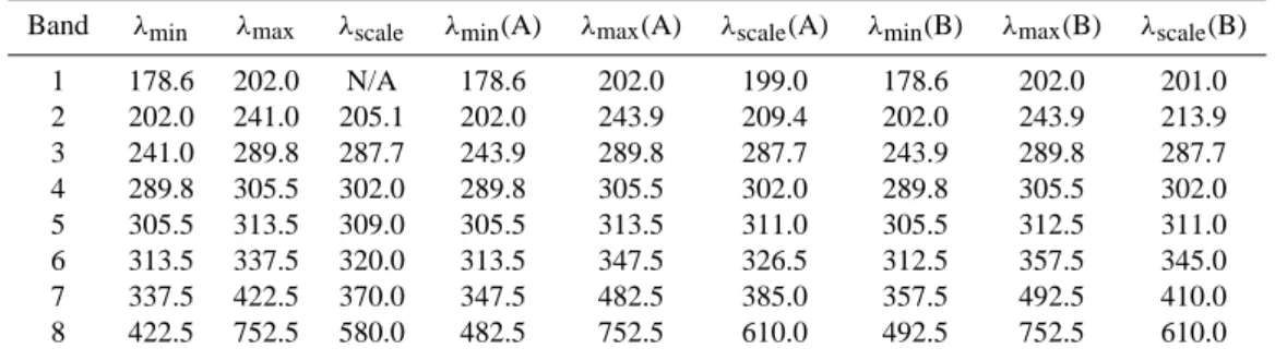
Table 1. Wavelengths chosen for the lower and upper band limits, and for the derivation of scaling ratios (δi)in the operational version of
the modified band approach. Values for θ <72◦are taken from Landgraf and Crutzen (1998) and those for θ =72–85◦(A) and θ =85–93◦(B) as derived in this study.
Band λmin λmax λscale λmin(A) λmax(A) λscale(A) λmin(B) λmax(B) λscale(B)
1 178.6 202.0 N/A 178.6 202.0 199.0 178.6 202.0 201.0 2 202.0 241.0 205.1 202.0 243.9 209.4 202.0 243.9 213.9 3 241.0 289.8 287.7 243.9 289.8 287.7 243.9 289.8 287.7 4 289.8 305.5 302.0 289.8 305.5 302.0 289.8 305.5 302.0 5 305.5 313.5 309.0 305.5 313.5 311.0 305.5 312.5 311.0 6 313.5 337.5 320.0 313.5 347.5 326.5 312.5 357.5 345.0 7 337.5 422.5 370.0 347.5 482.5 385.0 357.5 492.5 410.0 8 422.5 752.5 580.0 482.5 752.5 610.0 492.5 752.5 610.0
the strong absorption by O2 in the spectral range λ=178.6–
202.0 nm, the contribution to Factby scattering in this
spec-tral range is assumed to be negligible for θ <72◦. However,
for λ≥202 nm, the scattering by gaseous molecules can make a significant contribution to Fact and, therefore, must be
ac-counted for. Moreover, for λ ≥300 nm the scattering con-tribution made by both aerosols and clouds must also be ac-counted for. Landgraf and Crutzen (1998) have shown that the J value for species X may be approximated by multiply-ing the Jabsvalue, calculated in a non-scattering atmosphere,
by a scaling ratio:
δi = Fact(λi) Fabs(λi)
(2) at a specific wavelength (λi)within the band limits for band
(i). Here Fact(λi)is the actual actinic flux at λiand Fabs(λi)
the actinic flux for a non-scattering atmosphere at λi. For
the accurate derivation of Fact in any chosen model
atmo-sphere both the single and multiple scattering components of the incident light have to be taken into account. For this purpose several numerical methods are currently available which provide an accurate solution to the radiative transfer problem, where many use a multiple-stream approximation of the diffuse intensity field (e.g. Lenoble, 1985). Although such methods are commonly employed for the simulation of accurate photolysis rates in lower scale models, their use in CTM’s is limited due to the numerical effort which is needed being rather expensive. For this reason the original band ap-proach of Landgraf and Crutzen (1998) is commonly used in conjunction with a two-stream RT solver using a plane parallel geometry of the model atmosphere when applied for calculating photolysis rates (e.g. Lawrence et al., 1999).
Equation (3) describes Fabs (λ), which is calculated for
each individual wavelength bin assuming the transmission of light adheres to Lambert-Beer’s law. Therefore, it is depen-dent on the slant column depth due to both absorbance by O3
and O2(τslant(λ)), with F0(λ) being the spectral solar
irra-diance at the top of the atmosphere. The absorption due to other trace gases (e.g. NO2), aerosols and clouds is assumed
to be negligible compared to that of O2and O3and is
there-fore ignored.
Fabs(λ) = F0(λ)e−τslant(λ) (3)
For a plane parallel geometry the slant optical depth (τslant
(λ)) can be calculated using the density profile ρO2 and ρO3
of oxygen and ozone and their associated absorption cross-sections σO2 and σO3: τslant(λ) = 1 µo X x=O3,O2 zTOA Z o ρxσ (λ)xdz (4)
where µ0 is the cosine of the solar zenith angle and TOA is the top of the atmosphere. This resulting Fabs(λ) is then used
for the calculation of Jabs, whose cumulative sum within a
band (i) is subsequently scaled by δi for the determination
of Ji. The scaling ratio (δi)need only be calculated for one
specific wavelength bin in each of the bands 2–8 and, thus, the full solution of the radiative transfer equation only needs to be performed for a total of 7 distinct wavelength bins. This makes the approach very efficient, as the most computation-ally expensive step in the derivation of Factis the calculation
of the scattering component. The Jxvalue is then calculated
by summing all Ji values for species X for all bands:
Jx=J1,xabs+ 8
X i=2
Ji,Xabsδi (5)
The main assumption used in the band model is that the Fact
in each spectral band scales linearly with the correspond-ing flux for a non-scattercorrespond-ing atmosphere. The scalcorrespond-ing lengths are chosen such that the errors made at shorter wave-lengths cancel out with errors made at longer wavewave-lengths for a chosen band i.e. the cumulative integral of all errors within such a band interval is approximately zero. In addition bi-ases in the individual band contribution can cancel out due to the summation in Eq. (5). This approach works very well for
4140 J. E.Williams et al.: Online photolysis in Chemical Transport Models
3 The modified band approach
In order to extend the original band approach for low sun geometry four main modifications have been applied to the existing scheme, as follows: (1) the radiative transfer model has to be extended to account for the spherical shape of the model atmosphere. For this purpose we introduce a pseudo-spherical extension of a two-stream method, where the sphericity is only accounted for in the calculation of the direct light component. The diffuse component of the radia-tion field is still considered in plane parallel geometry. (2) A limit is applied to the scaling ratios (δi)for instances where Fabsfalls below a selected threshold value. (3) A scaling
ra-tio is introduced for the first band (λ≤202 nm) taking into account the scattering of radiation in the upper part of the model atmosphere. (4) Due to the increase of the slant optical depth (τslant)in instances of low sun, the maximum amount
of radiation per band interval is shifted towards wavelengths of weaker absorption. Therefore, for high incident angles the selection of the scaling wavelengths (λi)and band limits
have been further optimized.
3.1 The model atmosphere and spectroscopic data
The development and testing of the modified band approach was performed using a standard one-dimensional column model atmosphere. The vertical grid consisted of 80 equidis-tant layers of 1km depth from the ground level to the top of the atmosphere. The pressure, temperature, relative hu-midity and O3concentrations were taken directly from the
U.S. standard atmosphere (NOAA, 1976) and interpolated onto the vertical grid. The total ozone column is scaled to 300 DU to allow direct comparisons with the results pre-sented in Landgraf and Crutzen (1998). The slant column for each layer/level combination is calculated in a similar manner to that documented by Madronich (1987) and is im-perative for the correct Fabsvalues in the lowest layers (and
thus scaling ratios). The ground was treated as a Lambertian reflector using fixed albedo values of 5% unless stated oth-erwise, with the value of the albedo being fixed across the entire spectral range.
Table 2 provides a comprehensive list of all of the pho-todissociation rates which have been examined during the testing phase. The characteristic absorption co-efficients (σx)and quantum yields (φx)for each chemical species (X) were taken from the latest recommendations (e.g. Sander et al., 2003; Atkinson et al., 2004) and subsequently interpo-lated onto the working spectral grid of Br¨uhl and Crutzen (1988), where 142 spectral bins are used between 178.6– 752.5 nm (of varying resolution). The number of photolysis rates added for stratospheric species has been significantly increased compared to the original treatise of Landgraf and Crutzen (1998) meaning that the performance of the both the original and modified band method is being tested for such compounds for the first time (e.g. BrO).
To avoid an exhaustive analysis involving all 38 photoly-sis reactions for which the approach was tested, we define two smaller subsets of the species with each subset being photolytically relevant to either the stratosphere or the tropo-sphere, as defined in Table 3. One of the conditions involved in the selection of these two chemical subsets was that the ab-sorption behavior was sufficiently diverse enough to be able to test the modified band method across the entire spectral range.
For molecular O2the absorption in the Lyman-Alpha and
Schumann-Runge regions of the spectrum are accounted for using the parameterizations of Chabrillat and Kockarts (1997) and Koppers and Murtagh (1996), respectively. For the photolysis of NO, which occurs in the far UV, the param-eterization of Allen and Frederick (1982) is implemented. Temperature dependencies of σ values are included for 18 of the chosen chemical species (see Table 2). Moreover, a temperature dependency for the φ related to O1D production from the photolysis of O3was also included as recommended
by Matsumi et al. (2002). For the calculation of the Rayleigh scattering cross-sections the empirical approach of Nicolet (1984) is used. To treat aerosols in the model atmosphere we use the optical properties described by Shettle and Fenn (1979) for a rural, urban, maritime and a tropospheric back-ground aerosol. The vertical distribution is adopted from Mc-Clatchey et al. (1972). The contribution of both absorption and scattering introduced by cloud layers is calculated using the parameterization of Slingo (1979). The model also al-lows one to take partial cloud coverage into account in the radiative transfer calculations using the approach of Geleyn and Hollingsworth (1979).
3.2 Spherical radiative transfer
To solve the spherical radiative transfer problem we consider a planetary atmosphere composed of homogeneous spheri-cal shells. The atmosphere is illuminated symmetrispheri-cally by parallel solar beams. Ignoring thermal emission and refract ional effects of radiation, the scalar RT equation is given by Eq. (6), (Chandrasekar, 1960; Goody and Yung, 1989):
dI
ds = −βextI + Jscat(I ) (6)
where the spectral intensity I is a function of position r and direction . βextrepresents the extinction coefficient, which
due to the symmetry of the model atmosphere depends only on the radius |r|. Furthermore the scattering source func-tion Jscat depends itself on the intensity field I . dsd is the
derivative along the pathlength s in the direction . Given the solution I , the actinic flux can be calculated by the solid angle integration:
Fact(r) =
Z
4π
dI (r, ), (7)
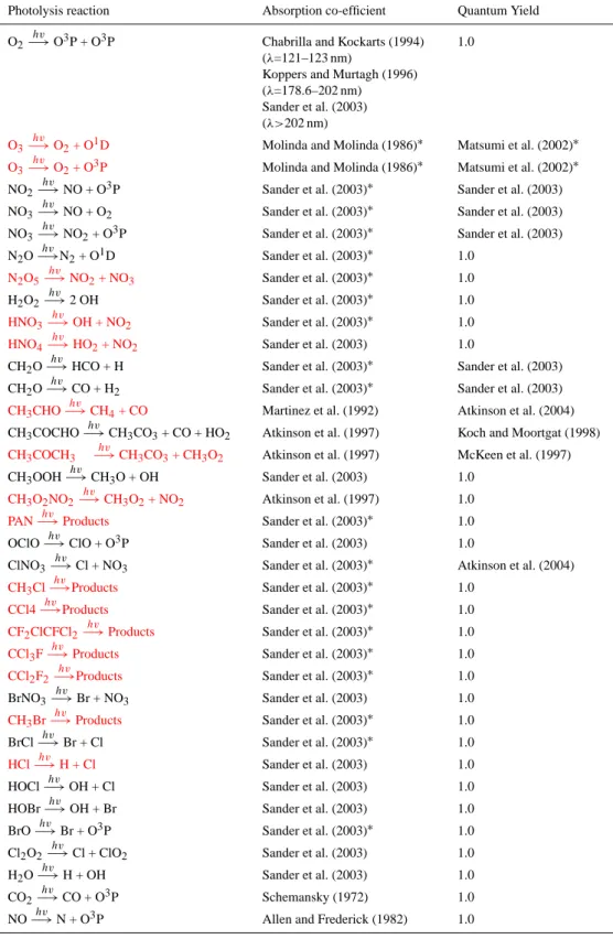
Table 2. Details concerning the literature values adopted for the characteristic absorption co-efficients and quantum yields for all photolyt-ically active chemical species evaluated in this study, where (*) denotes temperature dependent absorption parameters. A value of unity is assumed for the quantum yields of species where there is a lack of laboratory data. Reactions highlighted in red are those for which limits are applied to the δ ratios for band intervals 2 and 4 once θ >81◦. For θ >85◦limits are applied to all chemical species in order to avoid problems in the middle atmosphere.
Photolysis reaction Absorption co-efficient Quantum Yield
O2
hv
−→O3P + O3P Chabrilla and Kockarts (1994) (λ=121–123 nm)
Koppers and Murtagh (1996) (λ=178.6–202 nm) Sander et al. (2003) (λ>202 nm) 1.0 O3 hv
−→O2+ O1D Molinda and Molinda (1986)∗ Matsumi et al. (2002)∗
O3
hv
−→O2+ O3P Molinda and Molinda (1986)∗ Matsumi et al. (2002)∗
NO2
hv
−→NO + O3P Sander et al. (2003)∗ Sander et al. (2003) NO3
hv
−→NO + O2 Sander et al. (2003)∗ Sander et al. (2003)
NO3
hv
−→NO2+ O3P Sander et al. (2003)∗ Sander et al. (2003)
N2O hv −→N2+ O1D Sander et al. (2003)∗ 1.0 N2O5−→hv NO2+ NO3 Sander et al. (2003)∗ 1.0 H2O2−→hv 2 OH Sander et al. (2003)∗ 1.0 HNO3 hv −→OH + NO2 Sander et al. (2003)∗ 1.0 HNO4 hv −→HO2+ NO2 Sander et al. (2003) 1.0 CH2O hv
−→HCO + H Sander et al. (2003)∗ Sander et al. (2003) CH2O
hv
−→CO + H2 Sander et al. (2003)∗ Sander et al. (2003) CH3CHO
hv
−→CH4+ CO Martinez et al. (1992) Atkinson et al. (2004)
CH3COCHO
hv
−→CH3CO3+ CO + HO2 Atkinson et al. (1997) Koch and Moortgat (1998) CH3COCH3
hv
−→CH3CO3+ CH3O2 Atkinson et al. (1997) McKeen et al. (1997)
CH3OOH
hv
−→CH3O + OH Sander et al. (2003) 1.0 CH3O2NO2−→hv CH3O2+ NO2 Atkinson et al. (1997) 1.0
PAN−→hv Products Sander et al. (2003)∗ 1.0
OClO−→hv ClO + O3P Sander et al. (2003) 1.0 ClNO3
hv
−→Cl + NO3 Sander et al. (2003)∗ Atkinson et al. (2004) CH3Cl
hv
−→Products Sander et al. (2003)∗ 1.0
CCl4−→hvProducts Sander et al. (2003)∗ 1.0
CF2ClCFCl2
hv
−→Products Sander et al. (2003)∗ 1.0
CCl3F
hv
−→Products Sander et al. (2003)∗ 1.0
CCl2F2
hv
−→Products Sander et al. (2003)∗ 1.0
BrNO3
hv
−→Br + NO3 Sander et al. (2003) 1.0
CH3Br−→hv Products Sander et al. (2003)∗ 1.0
BrCl−→hv Br + Cl Sander et al. (2003)∗ 1.0
HCl−→hv H + Cl Sander et al. (2003) 1.0
HOCl−→hv OH + Cl Sander et al. (2003) 1.0 HOBr−→hv OH + Br Sander et al. (2003) 1.0 BrO−→hv Br + O3P Sander et al. (2003)∗ 1.0 Cl2O2
hv
−→Cl + ClO2 Sander et al. (2003) 1.0
H2O hv −→H + OH Sander et al. (2003) 1.0 CO2 hv −→CO + O3P Schemansky (1972) 1.0 NO−→hv N + O3P Allen and Frederick (1982) 1.0
4142 J. E.Williams et al.: Online photolysis in Chemical Transport Models
Table 3. Definitions of the tropospheric and stratospheric chemical subsets selected for the derivation of the low sun band settings and the analysis of the performance of the modified band approach. The spectral range indicates the spectral region over which each species exhibits absorption.
Troposphere Stratosphere
Photolysis reaction Spectral range [nm] Photolysis reaction Spectral range [nm] O3−→hv O2+ O1D 219.8–342.5 N2O−→hvN2+ O1D 178.6–241.0 NO2 hv −→NO + O3P 202.0–422.5 OClO−→hv ClO + O3P 259.7–477.5 N2O5 hv −→NO2+ NO3 178.6–382.5 Cl2O2 hv −→Cl + ClO2 178.6–452.5 HNO3−→hv OH + NO2 178.6–352.5 ClNO3−→hv Cl + NO3 196.1–422.5 HNO4 hv −→HO2+ NO2 178.6–327.9 BrNO3 hv −→Br + NO3 178.6–497.5 H2O2 hv −→2 OH 178.6–347.5 BrO−→hv Br + O3P 311.5–392.5 CH2O−→hv HCO + H 298.1–347.5 CCl2F2−→hv Products 178.6–241.0 CH2O hv −→CO + H2 298.1–357.5 BrCl hv −→Br + Cl 200.0-602.5
The spherical radiative transfer equation, as given in Eq. (6), represents a differential equation for three spatial pa-rameters. It can be solved by integration along a representa-tive set of the characteristic lines. In turn the intensity field (I) can be determined using a Picard iteration scheme. However, for the three-dimensional spatial problem a large number of characteristic lines are needed, which hampers any numeri-cal implementation. Here Rozanov et al. (2001) and Doicu et al. (2005) have shown that the number of characteristic lines can be reduced significantly using the symmetries of the model atmosphere and the solar illumination. In this study we utilize as a reference the model of Walter et al.1, which is based on this solution concept. The model has been veri-fied with comparisons made against Monte Carlo simulations for the reflected intensity field and has shown an agreement of better than 2% employing in total 2.4×10⁵characteristic lines. For the actinic flux within the atmosphere we expect a similar or even higher accuracy.
For the numerical implementation of an algorithm to cal-culate photolysis rates in a CTM we are heavily restricted by the computational burden which RT schemes introduce. For this reason we have chosen the RT solver called PIFM (Practical Improved Flux Method), which was originally de-rived by Zdunkowski et al. (1980) and uses a two-stream ap-proximation for calculating the diffuse components of Fact.
The generalized two-steam approximation of scalar radiative transfer, in its plane parallel geometry, may be expressed by Zdunkowski et al. (1980): 1 βext dF+ dz =α1F +− α2F−−α3Io (8)
1Walter, H.H., Landgraf, J., Spada, F., and Doicu, A., Lineariza-tion of a radiative transfer model in spherical geometry, J. Geophys. Res., submitted, 2006. 1 βext dF− dz =α2F +− α1F−+α4Io (9) µo βext dIo dz =Io (10)
Where F+and F−are the upward and downward fluxes and Io describes the direct solar intensity, z represents the
altitude, and the coefficients α1to α4are given by:
α1=U (1 − ω(1 − βo)) (11)
α2=Uβoω (12)
α3=ωβ(µo) (13)
α4=(1 − ω)β(µo). (14)
Here U is the diffusivity factor, ω is the single scattering albedo, βois the fractional mean backward scattering
coeffi-cient and β(µo)is the backward scattering coefficient of the direct solar beam. The values for the diffusivity factor and the backscattering coefficients depend on the particular two-stream approximation. The PIFM RT solver (Zdunkowski et al., 1980) utilizes the following parameters:
U =2 (15) βo= 3 − p1 8 (16) β(µo) = 1 2 − µo 4 p1 (17)
where p1is first coefficient of an expansion of the scattering
Equations (8–10) can be solved by using standard meth-ods for a vertically inhomogeneous atmosphere which is sub-divided into a number of homogenous layers. Using the solu-tion for F+, F−and Io, the actinic flux can be approximated
by:
Fact=U (F++F−) + Io. (18)
To take into account effects of the Earth sphericity on the ra-diative transfer one can use, as a first correction to the plane parallel approach, the air mass of a spherical model atmo-sphere for the attenuation of the direct beam. Therefore we modify the air mass factor (µ−o1)in Eq. (10) by a correspond-ing expression suggested by Kasten and Young (1989);
f (γ ) = 1
sin γ + a(γ + b)−c (19)
Where γ is the solar elevation angle and values for the em-pirical constants of a=0.5057, b=6.08◦, and c=1.636. We hereafter refer to this version of the solver as PIFM-KY.
A more sophisticated method of representing sphericity is the pseudo-spherical approximation (e.g. Caudill et al., 1997; Rozanov et al., 2000; Spur et al., 2001; Walter et al., 2004). Here the Lambert-Beers absorption law of the direct beam in Eq. (10) is replaced by a corresponding equation for spherical geometry:
dIo
ds = −βextIo (20)
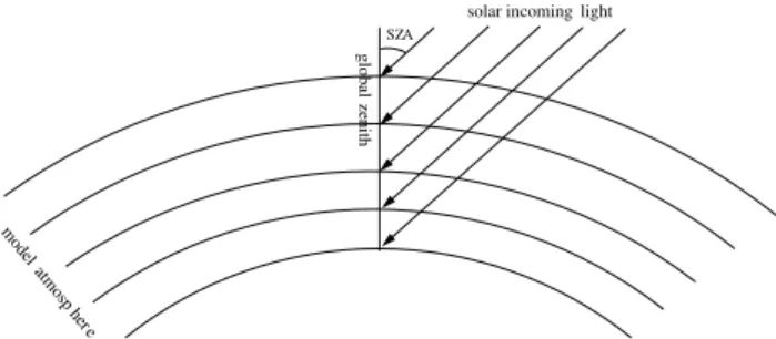
with s being the path length of the direct beam through a spherical atmosphere with respect to the global zenith angle. Figure 1 shows the slant path of the direct beam as it travels through such a spherical atmosphere. By solving this equa-tion, the direct light can be coupled into the flux equation of a plane parallel atmosphere via Eqs. (6) and (7). For θ >90◦, one has to bear in mind that the solar beam does not illu-minate the upper boundary of a particular atmospheric layer anymore but its lower boundary. In turn we have to modify the coefficients α3and α4in Eqs. (8) and (9), accordingly:
α3= [2(µo)ω + 2(−µo)(1 − ω)]β(µo) (21) α4= [2(−µo)(1 − ω) + 2(µo)ω]β(µo) (22)
where 2 is the Heaviside step function. These modified flux equations can subsequently be solved using the method de-scribed by Zdunkowski et al. (1980). We hereafter refer to this version of the solver as PIFM-PS.
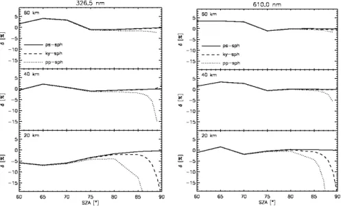
To give an estimate regarding the accuracy of both PIFM-KY and PIFM-PS, we have compared simulations of the actinic flux with those calculated using the spherical ref-erence model (hereafter referred to as refref-erence model A). Figures 2a and b show the percentage differences in
Fact obtained when comparing the plane parallel PIFM
model, PIFM-KY and PIFM-PS with reference model A at
λ=326.5 nm and λ=610 nm, respectively. For θ <70◦, the dif-ferent versions of PIFM provide almost identical results for
solar incoming light
global zenith SZA model atmosp her e
Fig. 1. Spherical geometry used for the pseudo spherical two-stream method. The solar radiation is calculated at the global zenith along its spherical light path through the atmosphere and then it is used as the source of solar light in a plane parallel atmosphere.
the chosen altitude levels, where differences compared with the reference model never exceed 5%. However, at θ >80◦ the simple plane-parallel model clearly deviates from the modified versions of PIFM, with the largest errors occurring at the lower altitudes (cf. 60 km with 20 km). Similar effects occur for θ >85◦using PIFM-KY. In contrast, these figures show that the pseudo spherical PIFM model provides very accurate estimates of the actinic flux up to θ =90◦. It should
be noted that PIFM-PS is much more computationally expen-sive than the PIFM-KY meaning that it’s application is only warranted when the increase in accuracy is significant (i.e.) above 85◦. Details relating to the computational expense of each version of the solver are discussed later in Sect. 5.
Figures 3 and 4 show the accuracy of PIFM-PS for θ =91– 95◦ as a function of altitude. At 326.5 nm the actinic flux decreases significantly between 20–60 km altitude due to the attenuation of the direct beam by Rayleigh scattering and ozone absorption. For this wavelength the actinic flux starts to decrease already at higher altitudes for higher incident an-gles, due to the longer path of the direct light through the atmosphere. At 610.0 nm the direct beam is much less atten-uated, which results in a less marked decrease in the Fact
with respect to altitude. For this wavelength the Fact
de-creases to very small values in the shadow of the Earth body, where only the diffuse component of the radiation is present. The PIFM PS solver can reproduce this feature very well and overall the corresponding errors are small. Only at altitudes where the contribution of the direct beam to Fact is
negligi-ble because of either the strong extinction which exists in the photon path or due to the shadow of the Earth body does the error increase to up to ±30%. However, due to the small values of Fact at these altitudes this large error is of minor
importance for our application. It should also be noted that an upper threshold of θ =93◦is used during the application of PIFM-PS following Lamago et al. (2003).
The subsequent error introduced into the final J values as a result of using PIFM to calculate Fact in Eq. (1) has
been studied by Landgraf and Crutzen (1998) and is, on av-erage, ∼5% for clear-sky conditions and ∼20% for cloudy
4144 J. E.Williams et al.: Online photolysis in Chemical Transport Models
Figure 2: Percentage differences (δ) in the actinic flux (Fact) calculated with different
model versions of PIFM versus a full spherical radiative transfer model as a function of the solar zenith angle (SZA). Differences in Fact are shown for comparisons between the
plane parallel PIFM version (pp), the version using the Kasten and Young correction for spherical air mass factors (ky) and the pseudo-spherical extension of PIFM (ps) versus reference model A (sph) at 20, 40 and 60 km altitude. The left panel shows differences for λ = 326.5 nm and the right panel for λ = 610.0 nm, which are pertinent to the scaling wavelengths chosen for grid A (see Table 1). The model atmosphere is adopted from the US standard atmosphere 1976, albedo = 0% and the total ozone column scaled to 300DU.
Fig. 2. Percentage differences (δ) in the actinic flux (Fact)calculated with different model versions of PIFM versus a full spherical radiative transfer model as a function of the solar zenith angle (SZA). Differences in Factare shown for comparisons between the plane parallel PIFM version (pp), the version using the Kasten and Young correction for spherical air mass factors (ky) and the pseudo-spherical extension of PIFM (ps) versus reference model A (sph) at 20, 40 and 60 km altitude. The left panel shows differences for λ=326.5 nm and the right panel for λ=610.0 nm, which are pertinent to the scaling wavelengths chosen for grid A (see Table 1). The model atmosphere is adopted from the US standard atmosphere 1976, albedo=0% and the total ozone column scaled to 300 DU.
Fig. 3. The Factat 326.5 nm as a function of altitude for θ =91–95◦ (left panel) and the associated error when comparing the PIFM-PS with reference model A (right panel). The model atmosphere is the same as in Fig. 2.
conditions for θ ≤60◦, as compared to the 32-stream discrete
ordinate code of Stamnes et al. (1988). The maximum errors occur in the middle troposphere where the contributions due to multiple scattering are the greatest.
For the PIFM-PS solver the subsequent error introduced into the final J values also needs to be quantified at high in-cident angles. Due the high computational effort involved in using reference A, the calculation of J value profiles using full spherical geometry was not possible within a reasonable
Fig. 4. Same as Fig. 3 but for 610.0 nm.
time. Therefore, in order to quantify the error in the resulting
Jvalues, we have interpolated the height resolved difference between actinic flux calculations performed using reference model A and PIFM-PS, which were calculated for the scaling wavelengths chosen for grid A (see Table 1), onto the work-ing grid of Br¨uhl and Crutzen (1988) for all 80 atmospheric layers. Subsequently we have scaled the PIFM-PS calcula-tions on the working grid of Br¨uhl and Crutzen (1988) with these error estimates to get a reliable estimate of the percent-age error introduced into Fact. In turn we are able to estimate
the corresponding errors in the J value profiles at any partic-ular zenith angle.
Fig. 5. Percentage errors associated with the J value profiles calculated using the PIFM-PS model as compared with reference model A at θ=90◦. For details regarding how the error was calculated the reader is referred to the text. Results are presented for (a) the stratospheric and (b) tropospheric chemical subsets, respectively. The model atmosphere is adopted from the US standard atmosphere 1976, albedo=0% and the total ozone column scaled to 300 DU.
Figures 5a and b, show the associated errors due to PIFM-PS at θ =90◦ for both the stratospheric and tropospheric chemical subsets, respectively. These figures show that the errors for the first 40 km of the column are generally of the order of ±2%. Below this height the error increases substan-tially for species such as N2O, although the actual J value
at this altitude is extremely small. For the other tropospheric species the errors down to 25 km are below ±5%, after which negative errors exist for all species. Fortuitously, the J val-ues become rather irrelevant at such high zenith angles in the lower portion of the column meaning that the effect on the overall performance of the PIFM-PS is minimal.
Figure 6 shows the corresponding errors for the worst case scenario of θ =93◦. Again, the associated errors in the J val-ues for the top 40km due to PIFM-PS were ±2%, except for
JN2O. Below this height there is so little direct flux (Fabs)
be-low 320 nm which penetrates through to the be-lower levels that the Fact for this spectral region is determined almost purely
by scattering. Therefore, the contributions by bands 1 to 4 subsequently decrease, resulting in lower errors in the J val-ues for the lowest 20km of the column compared to θ =90◦.
It should be noted that the effects of atmospheric refrac-tion of the solar beam were not included in either reference model A or the PIFM-PS solver. To do so would involve a significant update to the reference code which is beyond the focus of this paper. Moreover, an iterative scheme would need to be introduced into the PIFM-PS solver for the deriva-tion of a modified solar zenith angle for each respective level, which would significantly increase the computational burden of the solver. Although the effects on certain free radical species can be significant between 40–50 km when
integrat-ing over a period of 7 days, the overall effect on O3is thought
to be relatively small (Balluch and Lary, 1997). Therefore, we feel that the error introduced into the calculation of height resolved Fact is not dominant compared to the other
uncer-tainties in (e.g.) the absorption characteristics for important chemical species such as Cl2O2(Sander et al., 2003).
In summary, the modification to the two-stream approxi-mation reduces the error introduced by using the two-stream approximation significantly, especially at the altitudes impor-tant during instances of very low sun (θ >90◦).
3.3 The scaling ratios (δi)
The most important assumption made in the band approach is that the Factscales with its direct component (Fabs)within
a specific wavelength band at any altitude, where the scal-ing ratio is assumed to be wavelength independent within a spectral band. This assumption has enhanced importance when the amount of incident radiation varies strongly within a spectral band (e.g. band 4). For such instances the approach only holds for situations where the diffuse radiation is gov-erned by the direct component due to the single scattering contribution of solar light at the same altitude. In instances where the diffuse component is scattered from other parts of the atmosphere this approximation breaks down. Such conditions are encountered for low sun at wavelengths which exhibit strong to moderate O3absorption (<305 nm),
result-ing in a direct flux in the lower atmosphere which is very small. For such a case the diffuse radiation mainly originates from scattering which occurs at higher altitude levels. Thus it would be more appropriate to use the scaling ratio calcu-lated at higher altitudes for the lower levels. However, for the
4146 J. E.Williams et al.: Online photolysis in Chemical Transport Models
Fig. 6. As for Fig. 5 except the θ =93◦.
Table 4. The flux thresholds adopted for Fabsduring the calculation of the scaling ratios for bands 2 through to 4 at θ >81◦. The ratio for Fabs/F0is given using photons nm−1s−1for the original fluxes. These ratios hold for the scaling wavelengths given in Table 1.
Band θ: 81–85◦ θ: >85◦ 2 1.2×10⁻⁴ 1.2×10⁻⁴ 3 No limit 4.5×10⁻¹² 4 2.7×10⁻⁵ 1.35×10⁻⁶
numerical implementation we apply a limit on the resulting scaling ratios whenever Fabsfalls below a selected threshold
value, which effectively means using a δi value calculated
for higher altitudes. The diagnostic used for the derivation of these Fabsthresholds was the occurrence of large associated
errors on the most sensitive J values accompanied by cor-respondingly high δi values. In general, it was found that δi values greater than 10 resulted in an overestimation of
the resulting band contribution to the final J values. For species which exhibit strong absorption characteristics for
λ<320 nm (e.g. O3, HNO3)it was found that such limits
are needed for θ >81◦ in order to reduce the associated
er-ror budgets. These were applied to bands 2 and 4 for the species highlighted in red in Table 2. Once the θ >85◦such
limits were applied for band intervals 2 through to 4 for all chemical species, using the (Fabs/Fo)ratios given in Table 4.
It should be noted that the ratios for these limits change for certain bands for incident angles above and below θ =85◦as a consequence of using PIFM-PS at θ >85◦, which modifies the Fabscomponent. No limits were applied to bands 1 or 5
through to 8 under any circumstances. For bands 6 through to
8 a sufficient amount of direct light penetrates through to the lower layers so as to ensure that the main assumption used in the band model never fails, even at high zenith angles.
A further modification to the band approach is the intro-duction of a scaling ratio for the first band. An assumption is made in the original band approach that absorption dom-inates for λ≤202 nm. This assumption only holds when the single scattering contribution to Fact can be neglected
com-pared to Fabs. Here the single scattering contribution from
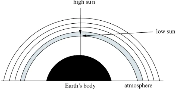
a certain model layer scales with the transmission of the at-mosphere located above that layer and the amount of radi-ation deposed in the model layer. Furthermore, the single scattering contribution is proportional to the single scattering albedo. However, this term does not depend on solar geome-try. For θ <70◦the single scattering contribution is insignifi-cant because the fraction of radiation deposed in the specific model layer is small and, in combination with the low single scattering albedo higher up in the atmosphere, results in the scattering of light being relatively unimportant. For lower sun, the path length of the solar beam through a model layer increases markedly which enhances the fraction of radiation deposed in each atmospheric layer. Figure 7 highlights this by showing the relative distance over which a photon must travel (the slant path) to an atmospheric layer which has been chosen in the model atmosphere for two different incident zenith angles. Therefore, for large slant paths, the scattering contribution becomes a significant part of the total flux in the upper part of the atmosphere. For this reason, it is necessary to use a scaling ratio for θ >72◦ for the first spectral band which accounts for this behaviour.
low sun high su n
Earth’s body atmosphere
Fig. 7. The variation in the slant path over which a photon has to travel to reach a particular layer (highlighted in grey) in the model atmosphere. For high sun a large amount of radiation can reach the top of this model layer. However, due to the relatively short pathlength of the solar beam through the layer, there is no signifi-cant contribution of singly scattered light in this model layer. For low sun the amount of direct light illuminating the top of the high-lighted layer is less as a consequence of the longer light path. How-ever it can be still sufficient to cause a significant contribution of singly scattered light in the model layer below in conjunction with the relatively large pathlength through the grey model layer for this geometry.
3.4 Selection of the band limits
Due to the shift of the amount of radiation towards longer wavelengths in instances of low sun, the band settings of Landgraf and Crutzen (1998) have to be modified for the band approach to maintain optimal performance at high in-cident zenith angles. Figure 8 shows the relative actinic flux
t (λ) = Fact(λ)/Fo(λ)at 10 km altitude between 300–320 nm,
normalized to the corresponding value at 310 nm, across a range of solar zenith angles. Here the actinic flux below 310 nm decreases relative to the centre wavelength with re-spect to solar zenith angle, whilst increases occur for wave-lengths above 310 nm. In other words, the relative amount of radiation is shifted towards longer wavelengths for larger solar zenith angles due to the longer path length of the di-rect beam through the atmosphere. This effect holds at this particular altitude until a θ =80◦, after which the shift in ra-diation towards longer wavelengths becomes weaker. This can be explained by the presence of the stratospheric ozone layer in combination with the spherical shape of the atmo-sphere. This behaviour is not seen for layers above the ozone layer or when adopting the plane parallel approximation of the model. In turn, the band limits and δi values of the
band model become non-optimal, which subsequently results in errors of between 10–30% which generally occur in the lowest 10km of the atmosphere for important tropospheric species (e.g. JH2O2)when the θ >80
◦.
An optimalization of the band settings for low sun is lim-ited by the requirements that the scheme should calculate height resolved J values for a diverse range of species over
Fig. 8. Relative actinic flux t (λ)=Fact(λ)/Fo(λ) between 300–
320 nm, normalized to the corresponding value at 310 nm, as a func-tion of solar zenith angle at 10 km altitude. For details regarding the model atmosphere the reader is referred to Sect. 3.1. Calculations were performed using the original band settings in conjunction with the original input parameters for the temperature dependent σ and
φof O3. The total ozone column was scaled to 300 DU and the ground albedo=5%.
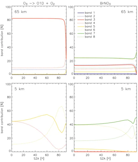
the entire model atmosphere. Moreover, the percentage con-tribution by each band to each J value is also dependent on height for many chemical species. Figure 9 shows an exam-ple of this effect, where the variation in the percentage con-tributions made by each spectral band to JO3(→O
1D) and
JBrNO3 is shown with respect to the zenith angle, for clear
sky conditions at two model layers situated at 65 and 5 km. These contributions are derived using the original band set-tings as given in Table 1. For the layer at 65 km it can be seen that JO3(→O
1D) is principally determined by contributions
originating from band 3, which contains the absorption max-imum for O3. In contrast, due to the overhead O3column
being relatively low at this altitude and the broad absorption characteristics of BrNO3, contributions are made to JBrNO3
across the entire spectral range i.e. bands 1 to 8. Moreover, the contribution made by each band to JBrNO3 only changes
marginally as the zenith angle increases until θ ≈90◦. How-ever, nearer the ground the percentage contributions made by each band change considerably as a consequence of the effective screening of the far UV by molecular O2 and O3.
This screening results in the contributions made by bands 1 through to 3 to be extremely small in the lower layers, result-ing in a decrease in the J values with respect to height. As the value of JO3(→O
1D) in the lower layers decreases with
increasing zenith angle (not shown), the percentage contri-bution made by band 4 also decreases (with an associated increase in the percentage contribution made by band 6) un-til θ =80◦. For θ >80◦the contribution made by band 4 at this particular altitude starts to increase again due to the spheric-ity of the Earth’s atmosphere. At these geometries the path length of the direct beam through the ozone layer decreases
4148 J. E.Williams et al.: Online photolysis in Chemical Transport Models
Fig. 9. The percentage contributions made by each spectral band for the calculation of JO3→O 1D and J
BrNO3at 5 and 65 km using the band
method. These contributions were determined using the original band settings taken from Landgraf and Crutzen (1998). The total ozone column was scaled to 300 DU and a ground albedo=5%.
with an increasing solar zenith angle. In turn, the relative amount of radiation is shifted towards shorter wavelengths, which increases the contributions made by bands 4 and 5. As a result, there is a corresponding decrease in the percent-age contribution made by band 6 to JO3 (→O
1D). The
ac-tual percentage contributions are weighted by the absorption characteristics of molecular O3. For JBrNO3 a similar effect
is observed near ground level, where the contributions from bands 1 through to 5 are screened out meaning that JBrNO3
is principally determined by the contributions from bands 6 through to 8. The optimialization of the band limits is ham-pered by such height dependent contributions from different bands, meaning that large associated errors maybe easily in-troduced into the J values in either the stratosphere or tropo-sphere if one does not assess the error throughout the entire column.
For the determination of the band parameters for θ >72◦ various combinations of λ(i)min, λ(i) and λ(i)max were
tested and the resulting errors in the J values assessed to discern whether any significant reduction in errors occurred compared to the original band settings. A limitation was found to exist in the choice of band limits for band 4 due to many of the species in the tropospheric subset exhibit-ing strong absorption in the spectral range covered by this band. Therefore, the resulting errors for such species were very sensitive to where the limits for this band were placed on the spectral grid. For bands 5 to 8 it was found that the ac-curacy of the method was increased by shifting the band lim-its and λ(i) towards the visible end of the spectrum, although
λ(8)maxremained unchanged. This procedure was performed
for the zenith angle ranges θ =72–85◦and θ =85–93◦, result-ing in parameter grids A and B, respectively (see Table 1). A criterion used for the selection of the optimal band settings was that the errors introduced by the band approach should not be greater than ±10% for the majority of the chemical species. Additionally, the errors should decrease compared
to those obtained using the original band settings for almost all of the chemical species. These grids were used for the cal-culation of all J values listed in Table 3, with the exception of
JNO, for the specified ranges of θ . For JN Ocontributions are
only made for a few of the wavelength bins in band interval 1 (Allen and Frederick, 1982) which were summed explicitly outside of the band limits
4 Assessment of the performance of the modified band approach
In this section we assess the performance of the band ap-proach using the optimalized band settings (grid A and B in Table 1) and compare the resulting errors with those calcu-lated using the original band settings. A range of atmospheric conditions have been chosen which are thought to cover the most important cases found in a CTM. The chemical subsets defined in Table 3 are used for this purpose. Moreover, for further brevity we limit the discussion below to the errors introduced when using a “final working version” of the mod-ified band approach. This “final working version” was the re-sult of several upgrades made to the fully explicit code driven by the need to remove the most computationally expensive interpolation steps. Therefore, a look-up table for the tem-perature dependent absorption parameters (namely σ and φ values) was produced using a resolution of 5◦C over the tem-perature range 180–340◦C and indexed using the temperature of each atmospheric layer. Various look-up tables with dif-fering resolutions between 1–10◦C were tested (not shown) and the 5◦C resolution found to be both accurate and
con-cise. Comparisons are made versus a version of the model which calculates Fact explicitly for each wavelength bin of
the working spectral grid of Br¨uhl and Crutzen (1988), with-out the use of a look-up table for the temperature dependent absorption parameters (hereafter referred to as reference B). It should be noted that both the “final working version” and reference B both use either PIFM-KY or PIFM-PS to cal-culate Fact values for ranges of θ above and below θ =85◦,
respectively. As a result, the following comparison pertains to the cumulative error introduced by both the modified band method and by the use of offline look-up tables for the σ and
φparameters.
4.1 Clear-sky and aerosol free conditions 4.1.1 Errors for θ =72–85◦
In this section we investigate the performance of the modified band approach under clear sky conditions over the range of
θ=72–85◦using grid A and present errors for certain species chosen from both the stratospheric and tropospheric subsets of chemical species.
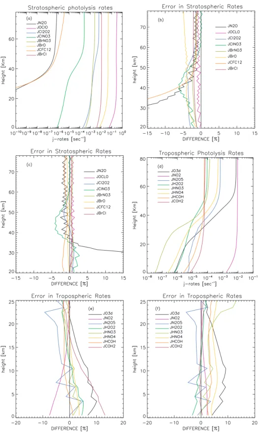
Figures 10a and d show the typical variation in J values, with respect to height, for both the stratospheric and tropo-spheric chemical subsets, respectively, under clear sky
condi-tions at θ =80◦and assuming an albedo of 5%. These profiles
were calculated using the “final working version” of the pho-tolysis scheme in conjunction with the original band settings (cf. Table 1). Figures 10b and e show the resulting errors as for the stratospheric and tropospheric chemical subsets com-pared with reference model B, respectively. The saw-tooth feature, which is evident in the error diagrams for certain species, is due to the use of the look-up table for the tem-perature dependent σ values (cf. the smooth error profiles which exist for species that have no temperature dependen-cies). The corresponding errors when using grid A are shown in Figs. 10c and f, respectively. By comparing the appropri-ate figures it can be seen that the application of grid A leads to substantially lower errors for both chemical subsets, espe-cially for BrO, CFC12, HCHO and H2O2, where the error is
approximately halved. It should be noted that the increase in the associated error for both JN2O and JCFC12 below 40km
relates to J values that are very small which tends to amplify the error introduced by small differences.
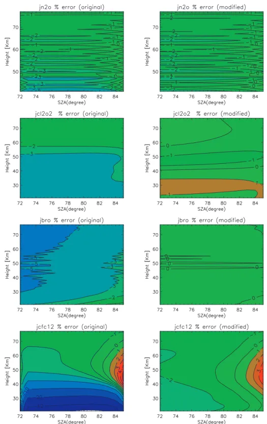
Figures 11a–h show the resulting contour plots for the variation in the error budgets with respect to incident zenith angle when using both the original and modified band ap-proaches. The corresponding contour plots for the tropo-spheric chemical subsets are shown in Figs. 12a–p, respec-tively. To aid comparison the results obtained using both band settings are placed side-by-side. By comparing these figures it can be seen that there are substantial reductions in the errors obtained using the modified version of the band approach for both of the chemical subsets. For the strato-spheric subset only a small selection of the chemical species are shown, with the other species having associated errors of ±3% for both the original and modified version of the approach (although a reduction in error is always observed using grid A). For those included in Fig. 11 all errors are be-low 10% for the first 50 km of the column across the entire range of incident θ , with the exception of JCFC12. For this
case the error drops substantially in the middle atmosphere due the use of the scaling ratio for band 1 (the band limits are identical for band1 between the original grid and grid A – see Table 1). It is also interesting to note that for the origi-nal band settings as the incident zenith angle increases some chemical species exhibit a reduction in the associated error as the contributions by each band to the total J value change (e.g. JBrO, Fig. 11e).
For the tropospheric subset the resulting errors are larger for the bottom 25 km of the column, especially for the orig-inal band settings. The zenith angle at which the associated errors show a significant increase is θ =82◦, with the
excep-tion of JNO2 (Fig. 12c). This is due to an over-estimation of
the band contribution made by band 4 to the final J value when using the original method, as a consequence of a large
δi value (i.e. low Fabs, see Sect. 3.3) in conjunction with the
use of non-optimal band parameters. The most dramatic re-duction in the associated errors occurs due to the applica-tion of limits on the δi values as can be seen for O3 when
4150 J. E.Williams et al.: Online photolysis in Chemical Transport Models
Fig. 10. Typical J value profiles calculated for (a) the stratospheric and (d) the tropospheric subsets of chemical species at θ =80◦using a ground albedo=5%. The associated errors introduced by using the “final working version” of the code are also shown for the stratospheric subset when adopting (b) the original band settings as taken from Landgraf and Crutzen (1998) and (c) Grid A. All comparisons are made against reference model B. Plates (e) and (f) show the corresponding information for the tropospheric subset.
Fig. 11. The variation in the error budgets associated with the J values calculated using both the original and modified band approaches for (a) N2O, (b) Cl2O2, (c) BrO and (d) CFC12, with respect to the incident θ . Comparisons are made against reference B. Plots are shown for a clear-sky scenario, where the total ozone column was scaled to 300DU and a ground albedo=5% adopted.
comparing Figs. 12a and b (i.e. the reduction in error due to the use of grid A alone is limited to ±10%). Although some error is still introduced by applying such limits
(be-tween ±10–20% for the lowest 10 km, see Fig. 12b) the maximum error drops by an order of magnitude. A simi-lar reduction in the error budgets is also observed for HNO3
4152 J. E.Williams et al.: Online photolysis in Chemical Transport Models
Fig. 12. The variation in the error budgets associated with the J values calculated using both the original and modified band approaches for (a) O3→O1D, (b) NO2, (c) N2O5and (d) H2O2, with respect to the incident θ . Comparisons are made against reference B. Conditions are identical to those described for Fig 11.
and HNO4. However, the application of the limits across all
species results in a decrease in the accuracy of the modified
band method for species such as H2O2due to the
Fig. 12. Continued. The variation in the errors associated with the J values calculated using both the original and modified band approaches for (a) HNO3, (b) HNO4, (c) HCHO→HCO+H and (d) HCHO→CO+H2, with respect to the incident θ . Comparisons are made against reference B. Conditions are identical to those described for Fig. 11.
(not shown). Therefore, for θ ≤85◦, the use of such lim-its should be selective and tests made for each particular species included within the photolysis scheme. The species
for which a significant reduction in errors is observed due to the application of such limits are highlighted in red in the comprehensive list of photolysis reactions given in Table 2.
4154 J. E.Williams et al.: Online photolysis in Chemical Transport Models
Fig. 13. The variation in the errors budgets associated with J values for (a) OClO, (b) Cl2O2, (c) ClNO3, and (d) BrNO3with respect to incident θ for a clear-sky scenario using grid B. Comparisons are made against reference B. Results are shown for the range θ =85–93◦using the PIFM-PS solver. Conditions are identical to those described for Fig. 11.
The sensitivity of the band method to the values of σ and
φ can be elucidated by comparing Fig. 12a with Fig. 5 in Landgraf and Crutzen (1998). Here, the associated errors calculated for JO3 (→O
1D) are approximately double those
shown in the original investigation using the original band settings when no limits are applied to the scaling ratio. This arises from updating the method in which φ is determined (where the temperature dependent σ values originate from Molina and Molina (1986) in both cases). The original quan-tum yield was taken from the study of Talukdar et al. (1998), whereas the one adopted here was based on the recommenda-tion of Matsumi et al. (2002), which is a critical synthesis of many independent studies. This update leads to substantial differences especially in the contribution made by the fourth band to JO3 (→O
1D) and, more importantly, the
contribu-tion to the total J value made by each wavelength bin (not shown). From this it maybe concluded that the errors asso-ciated with the band method are critically dependent on the input parameters used to determine the individual photolysis
rates. Therefore, it should be noted that any future updates may affect the absolute values of the associated errors pre-sented here.
The effect of ground albedo on the resulting errors was tested for those photolysis rates which are most important near to the ground, as this is where the largest perturbation of the radiative flux occurs due to enhanced reflection. For all instances the surface was assumed to behave as a Lam-bertian Reflector. It was found that the performance of the modified band approach is fairly robust across the range of ground albedos from 0.01 through to theoretical maximum of 1.0, and, in general, the errors remain rather constant for the chemical species contained in the tropospheric subset. Therefore, it can be concluded that the modified band ap-proach can be used with confidence over a diverse range of reflecting surfaces.
Finally, as a means of testing the sensitivity of the band method to the variation in the total overhead O3column (i.e.
Fig. 14. The variation in the error budgets associated with the J values calculated using the modified band approach with grid A in the presence of tropospheric aerosol for (a) O3→O1D (b) HNO3(c) HNO4and (d) HCOH with respect to the incident θ . Comparisons are made against reference B. The contouring used is identical to Fig. 12 to aid comparison. All other conditions are identical to those described in Sect. 4.2.
various scaling factors of between 250–400 DU (not shown). No significant change in the distribution of the associated er-rors compared to those shown for 300 DU were observed, indicating that the performance of the band method is robust over a range of atmospheric conditions.
4.1.2 Errors for θ =85–93◦
For solar zenith angles >85◦, the magnitude of the F
act
val-ues in the middle and lower layers of the atmosphere (be-low 50 km) are essentially governed by the diffuse radiation i.e. the Fabs contribution becomes very small. As with
so-lar zenith angles <85◦, this has unwanted numerical conse-quences in terms of large values for the δi ratios calculated
for bands 2 through to 4, which results in unrealistically large
J values. Therefore, a limit for the scaling ratios was again applied to the bands 2 through to 4 between θ =85–93◦. Due to differences in the radiation field as a result of using
PIFM-PS (i.e. an increase in Fabs), a further set of limits for the
δi ratios are defined for θ >85◦as given in Table 4. For the
tropospheric subset of species, the values for Fact become
so small near the surface that the resulting J values become rather unimportant when considering the diurnally integrated rates. Thus, we limit the following discussion to the errors associated with the stratospheric subset of chemical species calculated when using grid B, in conjunction with the PIFM-PS solver. Figures 13a–d show the resulting errors calcu-lated for J values over the range θ =85–93◦for a select num-ber of species from the stratospheric chemical subset thought to be the most important for polar chemical ozone deple-tion at such high incident angles (Lamago et al., 2003). For the range θ =85–90◦a resolution of 1◦ is used, after which
a finer resolution of 0.5◦ is adopted to provide more infor-mation between θ =90–93◦. The associated error budgets are generally below 10% above 30 km altitude, except where the
4156 J. E.Williams et al.: Online photolysis in Chemical Transport Models shadowing effect of the earth begins to reduce the Fabs
com-ponent to such an extent that the application of limits to the scaling ratio is needed. This subsequently introduces larger errors of between 10–30% at 20–30 km. Moreover, the ap-plication of grid B leads to a substantial reduction in the as-sociated errors compared to J values calculated with both the original grid and grid A (not shown). Although it is pos-sible to calculate J values with PIFM-PS up to an incident zenith angle of 95◦(see Sect. 3.2), the small values of both
Factand Fabsresult in large errors being introduced at angles
above θ =93◦for similar reasons to those discussed above. In fact, a significant degradation in the performance can be seen for θ >92.5◦, suggesting this limit should be applied online. Moreover, many of the J values become so small under such conditions that the computational expense of performing the calculation is often not warranted.
4.2 Clear-sky with tropospheric aerosol
In global CTMs clear-sky conditions almost never exist due to the ubiquitous presence of aerosols, liquid water clouds and ice water clouds (with the cloud fraction, liquid water content and ice water content usually being defined by the meteorological input data). The effect of both clouds and aerosol on atmospheric processes via the perturbation of the radiation field has been extensively discussed in the litera-ture (e.g. He and Carmichael, 1999; Haywood and Boucher, 2000; Tie et al., 2004). Here we investigate the effects that aerosol particles have on the error budgets associated with the J values calculated with the modified band approach. For brevity we only present the results calculated using grid A for a few species selected from the tropospheric subset, which are thought to be the most sensitive. The simulations are performed using rural aerosol for the lowest 4km and ‘back-ground’ aerosol for the rest of the model atmosphere. The particle number density of each layer was scaled such that the integrated optical depth due to the aerosol column was 0.32 at 550 nm, in line with the settings chosen in Landgraf and Crutzen (1998). Figure 14 shows the effect of aerosol loading on the error budgets associated with the J value pro-files calculated for O3→O1D, (b) HNO3, (c) HNO4and (d)
HCOH. For this purpose comparisons are made against J value profiles calculated using reference model B. Compar-ing these contour plots with the correspondCompar-ing plots given in Fig. 12 shows that the contouring is approximately the same for these chemical species. Therefore, the additional absorp-tion and scattering introduced by tropospheric aerosol does not result in any significant degradation in the performance of the modified band approach.
For the “urban” aerosol, as defined by Shettle and Fenn (1979), which exhibits a higher absorption component than the “rural” aerosol, there is a larger reduction in the J val-ues for the bottom layers compared to those obtained using “rural” aerosol (not shown). However, the effect on the error
budgets is again minimal, meaning that no significant differ-ences exist compared to the error contours shown in Fig. 14. 4.3 Cloudy atmosphere
The final analysis presented in this paper focuses on effects of cloud on the error budget of the modified band approach. For this purpose we consider a model atmosphere with two cloud layers each having 100% cloud coverage at 1–2 km and 7–8 km with optical densities of 24.9 and 38.3, respec-tively. The aerosol loading is prescribed as in Sect. 4.2 but we assume that the relative humidity within the cloud layers is near saturation (98%). Due to the increase in relative hu-midity in the cloud layer the aerosol optical depth increases to 0.52 at 550 nm. Such conditions pertain to the type of scenarios commonly encountered in a CTM. For the tropo-spheric species the effect of cloud on the J values is similar to that shown in Landgraf and Crutzen (1998), and is briefly summarized here. The attenuation of light directly above the highest cloud layer (at 7–8 km) causes a substantial increase in the magnitude of the J values at the cloud top (∼50%). This amplification gradually disappears with altitude until the J values are approximately equal to clear sky conditions at ∼20 km altitude. There is a corresponding decrease di-rectly below the cloud layer (∼20%), which again gradually disappears at altitudes of 2–3 km. The lower cloud layer ef-fectively screens the lowest layers resulting in decreases in the certain J values of upto ∼80%. Those species which absorb below λ<320 nm are the most affected due to the im-portance of enhanced scattering in the UV spectral region.
Figure 15 shows the effect both cloud and aerosol has on the error budgets associated with the J values calculated for the chemical species shown in Fig. 14. Although there is a re-distribution and, in some instances, a change in the asso-ciated error budgets for a few of the species shown the result-ing errors are generally still within ±10% in the lower 10 km, even though the optical density of the column increases sig-nificantly. Moreover, it should be noted that this result per-tains to a worst-case scenario of 100% cloud coverage. In a CTM the majority of grid cells have smaller cloud fractions and thus, smaller changes in the associated errors compared to the full-cloud scenario. It should be noted that for θ >85◦ clear-sky conditions are assumed in PIFM-PS during the RT calculations due to the numerical instability introduced in the lower layers for combinations of long slant paths and layers with high optical depths due to abnormally high τslantvalues.
Figure 16 shows the corresponding results for the strato-spheric species included in Fig. 11. Comparison of these plots shows that the effect of the increase in upwelling ra-diation is rather insignificant. However, it should be noted that the J values for more sensitive species (e.g. NO2)can
be altered by this effect (not shown).
In summary, no significant degradation in the accuracy of the band method occurs for cloudy conditions for chemical