An improved matrix-based endovascular guidewire position simulation using fusiform ternary tree

HAL Id: hal-02887427

https://hal.archives-ouvertes.fr/hal-02887427

Submitted on 16 Jul 2020

HAL is a multi-disciplinary open access

archive for the deposit and dissemination of sci-entific research documents, whether they are pub-lished or not. The documents may come from teaching and research institutions in France or abroad, or from public or private research centers.

L’archive ouverte pluridisciplinaire HAL, est destinée au dépôt et à la diffusion de documents scientifiques de niveau recherche, publiés ou non, émanant des établissements d’enseignement et de recherche français ou étrangers, des laboratoires publics ou privés.

An improved matrix-based endovascular guidewire

position simulation using fusiform ternary tree

Jianpeng Qiu, Jianxiao Yang, Yang Chen, Shoujun Zhou, Liudong Xing

To cite this version:

Jianpeng Qiu, Jianxiao Yang, Yang Chen, Shoujun Zhou, Liudong Xing. An improved matrix-based endovascular guidewire position simulation using fusiform ternary tree. The International Journal of Medical Robotics and Computer Assisted Surgery, John Wiley & Sons, Inc., 2020, 16 (6), pp.1-11. �10.1002/rcs.2137�. �hal-02887427�

An improved matrix-based endovascular guidewire position simulation using

fusiform ternary tree

Jianpeng Qiu1,3#_{, Jian Yang}2#_{, Yang Chen}1,4,5,6_{, (SENIOR MEMBER, IEEE), Shoujun Zhou}3_{, Liudong} Xing7

1 _{Laboratory of Image Science and Technology, School of Computer Science and Engineering, Southeast University,}

Nanjing 210096, China

2 _{Beijing Engineering Research Center of Mixed Reality and Advanced Display, School of Optics and Photonics, Beijing}

Institute of Technology, Beijing 100081, China

3 _{Shenzhen Institutes of Advanced Technology, Chinese Academy of Sciences, Shenzhen 518055, China} 4 _{Centre de Recherche en Information Biomedicale Sino-Francais (LIA CRIBs), Rennes, F-35000 France}

5 _{Key Laboratory of Computer Network and Information Integration (Southeast University), Ministry of Education,}

Nanjing 210096, China

6 _{School of Cyber Science and Engineering, Southeast University, Nanjing 210096, China}

7 _{Electrical and Computer Engineering Department, University of Massachusetts, Dartmouth, MA 02747, USA}

#_{these authors contributed equally to this work and should be considered co-first authors.}

Corresponding Author: [Yang Chen]

[School of Computer Science and Engineering, Southeast University, Nanjing, China] [chenyang.list@seu.edu.cn]

[+86 18651623205] [Shoujun Zhou]

[Shenzhen Institutes of Advanced Technology, Chinese Academy of Sciences, Shenzhen, China] [sj.zhou@siat.ac.cn]

[+86 13924607927]

Keywords Guidewire simulation, Endovascular interventions, Fusiform ternary tree, Optimal path Abstract

In this paper, a new matrix-based method is proposed to real-time determine the guidewire position inside an arterial system. The guidewire path is obtained by the optimal path method, particularly, the fusiform ternary tree method according to the principle of minimum output value of root node. An adaptive sampling strategy, and an optimization strategy based on proximal end and distal end of the guidewire are proposed to change the guidewire position for obtaining an ideal guidewire path. Compared to the existing methods, the proposed method can achieve 74%, 64% and 70% improvements in accuracy for phantoms 1, 2, and 3 investigated in this work.

1 Introduction

Cardio-cerebrovascular disease is a common disease, which is characterized by high complications, high recurrence rate, high mortality, and high morbidity. Although the most advanced medical equipment and treatment methods, more than 50% of cardio-cerebrovascular accidents survivors are still unable to live independently. Interventional radiology [5], also known as interventional angiography, is a marginal discipline developed rapidly since late 1970s. It has been widely used to treat various cardiovascular and cerebrovascular diseases, such as arteriovenous malformation, malignant tumour, liver cancer and etc. A guidewire is usually a thin, soft metal wire, which can be implanted into a tortuous or narrow vessel to serve as a guide for subsequent implantation of a catheter or other devices. In a vessel phantom that simulates the real environment of human blood vessels, a guidewire is first inserted slowly into a predefined target position, a guidewire/surgicalpath is then obtained by manual or algorithmic extraction from the CT angiography, this guidewire/surgical path is finally reproduced (using a guidewire simulation algorithm) in clinical operation to better guide physicians, the above process is termed static guidewire simulation. Conversely, dynamic guidewire simulation refers to the process of slowly inserting the guidewire into the surgical simulator [2, 6, 8, 21] to reproduce the medical surgical path in a virtual environment, where this dynamic simulation process must contains a collision detection and a collision response. Besides, the static guidewire simulation tends to surgical path planning, while the dynamic guidewire simulation tends to core skills training for training surgeons. Therefore, it is very valuable to simulate the guidewire path for surgical path planning and core skills training.

Regarding dynamic guidewire simulation, many domestic and foreign scientific research institutions and commercial companies have made a lot of research results. For example, Xu et al. [31] presented a (1+ε)-approximate algorithm with theoretical guarantee to model the guidewire behavior, which was not suitable for simulating the complex guidewire behavior in 3D space. Zienkewickz et al. [36] proposed the finite element methods (FEM) to address interactions between interventional devices and the vascular system. In [7], a linear model based on the finite beam elements and the substructure decomposition was presented. Based on the method of [7], Lenoir et al. [16] developed a simulator to better model interactions between the guidewire and catheters. Konings et al. [1, 3, 13, 17] presented the connected beam element methods according to theoretical mechanics and Hooke’s law in 2003. Cardoso et al. [10] reported a novel method to simulate and to predict the guidewire and catheter path inside a blood vessel based on equilibrium of a new set of forces, which leads to the minimum energy configuration. Next, based on previous research results, Sharei et al. [11] performed a systematic mapping study on the guidewire models and other information in 2018, which was the first more complete literature review.

Regarding static guidewire simulation, some research works have also been done. For example, Schafer et al. [26, 27, 32] proposed a beam-like method [8, 20, 30] according to the FEM and the connected beam element methods. Additionally, some improved beam-like approaches have been used to some medical simulators, e.g., [2, 6, 8, 21]. Shen et al. [24] presented a regularized open snake model to extract a centerline of tubular object in the noisy image data. Besides, this model has been used in the surgical path planning of medical robots [25] and centerline extraction [28]. In [22], an iterative refinement algorithm was proposed to further obtain an ideal running time according to the ideas and methods of Chen et al. [14, 15, 34, 35].

All of the above-mentioned methods involve high computational cost and cannot achieve an ideal guidewire path within an acceptable running time. In [23], Qiu et al. can achieve an ideal guidewire path within an ideal running time. However, this approach failed to plan a surgical path well on proximal end and distal end of the guidewire. Meanwhile, the simulation result is poor in the place where the vessel curvature is large. To overcome these disadvantages, we presented a matrix-based method to simulate guidewire path. The main difference between the proposed method and Qiu et al. [23] is the different iterative refinement methods: in [23], the parameter

δ

(iterative refinement termination condition) tends to be assigned to a smaller threshold (e.g., 4), the merging small edge strategy of adaptive sampling is then used, while the proposed method tends to assign a bigger threshold to

δ

(e.g., 31), and then uses splitting big edge strategy of adaptive sampling.

behavior inside an arterial system. Compared with the previous method [22], the proposed method improves the iterative refinement procedure (i.e., cancel the parameter

α

(the number of maximum curvature points) and adopt an adaptive sampling strategy), and adopts the fusiform ternary tree approach as well as an optimization strategy based on proximal end and distal end of the guidewire by using a multi-thread technique to improve both running time and accuracy in simulations.

The remainder of this study is organized as follows: Section 2 presents the proposed model. Section 3 presents experiment evaluation and compares the proposed method with the previous methods. Section 4 discusses the experiment results. Section 5 gives conclusion and indicates research directions for future work.

2 Proposed Method

A matrix-based method is presented for simulating the behavior of a guidewire inside the artery, which contains the following main tasks. An iterative refinement process with an adaptive sampling strategy is firstly presented, where some ordered centerline points are achieved using the maximum curvature, and used in constructing the matrix. The adaptive sampling strategy is more precise to express the guidewire behavior. We then define an energy function to assign a value to each element of the matrix. Next, we will discuss how to construct some fusiform ternary trees to determine the optimal path. Finally, the multi-thread optimization strategy is described to optimize simulation results.

2.1 Iterative refinement algorithm

We denote the 3D guidewire centerline points by an ordered set

L

=

{

L

0,

...

,

L

|L|−1

}

, and represent the i-th point of the centerline by

L

i, where i is the centerline index (|L| is the size ofL, 0 ≤ i ≤ |L| − 1). Meanwhile, these centerline points are

used as the data input.

In [22], an iterative refinement approach was proposed but failed to accurately screen out some maximum curvature points. In this subsection, to remedy this disadvantage, we improve the approach by canceling the parameter

α

used in [22] and by adopting an adaptive sampling strategy. During an iterative refinement, a maximum curvature point between centerline pointsL1and

L

|L|−2is first identified, which is denoted by

L

musing the following function (1) [31].

(

5 5

)

1

cos

− −

⋅

+

=

i i i i L

L

L

L

L

C

i (1)

The maximum curvature points between

L

mandL1, and between

L

mand

L

|L|−2 are then identified, and so on. The

iteration continues until the distance of centerline indexes of any two adjacent points identified is less than a given threshold

δ

(iterative refinement termination condition). The indexes of the maximum curvature points generated during the iteration process constitute an ordered set B. Then, several maximum curvature points are identified from set B based on the adaptive sampling strategy (split big edges), which is defined in Section 2.2. Finally, we put centerline indexes of the maximum curvature points into this ordered set B.

The above iteration method can be described as follows: Step 1: Centerline index values of L1and

L

|L|−2are put into set B;

Step 2: A maximum curvature point is identified (represent by

L

m) betweenL1and

L

|L|−2 using (1), and put this

centerline index m into set B. Then, sort unordered set B using the bubble sort method, where index values of these points is the increasing order;

Step 3: In sorted set B, regarding any two points with continuous indexes (e.g.,

L

B[k]and

L

B[k+1]), if the distance

between

L

B[k]and

L

B[k+1]is more than a given constant

δ

(e.g., 30), then we screen out a maximum curvature

point (represent by

L

h) between them using (1). The index h is put into unordered set B. Then, sort the set B using

the bubble sort algorithm, where index values of these points are the increasing order. Repeat Step 3 until the interval of index values of any two continuous points in ordered set B is less than

δ

;

Step 4: Get another maximum curvature point between

L

B[k]and

L

B[k+1] by using (1) if the interval of

L

B[k]and 1]

k

B[ +

L

is more than a predefined constant

δ

'

(

δ

'

<

δ

), where B[k]+5 ≤ i ≤ B[k+1]-5, k=0...|B|-2. This point’s index

is then put into the ordered set B. Repeat Step 4 until the interval of index values of any two continuous points in ordered set B is less than a predefined constant

δ

'

(e.g., 15);

Step 5: Sort unordered set B using the bubble sort method; Step 6: Acquire |B| ordered 3D centerline points.

Illustrative programming Example:

Data input set L = {L0, …, L31}, and predefined parameter

δ

= 10 and

δ

'

= 8.

Step 1: Put 1 and 30 into initial set B;

Step 2: Calculate a maximum curvature point

L

23 between L1and

L

30. Then, put 23 into set B. After sorting, B = {1, 23,

30};

Step 3: Calculate one maximum curvature point

L

16 between

L

23 and L1. Then, calculate the other maximum

curvature point

L

11 between

L

16and L1. Finally, put 16 and 11 into unordered set B. After sorting, B = {1, 11, 16,

23, 30};

Step 4: Calculate a maximum curvature point

L

6betweenL1and

L

11since the distance between them is more than the

predefined constant

δ

'

. Then, put 6 into set B. After sorting, B = {1, 6, 11, 16, 23, 30}.

After the ordered set B is obtained using the above iterative method, we construct |B| meshes with each centerline point

L

B[k], where these meshes are described in detail in [32]. The vectorLB[k]−1LB[k]is denoted by centerline points

L

B[k]-1and

L

B[k]. Then, the meshMLB[k]perpendicular to LB[k]−1LB[k]is constructed according to this vector. Every meshMLB[k] comprises four circles, where m sampled points (e.g., 43) are evenly spaced across these circles. We denote

each sampled point as

m

i, LB[k], where i is index of each sampled point, and LB[k] is the index per mesh.

Next, this spatial representation is represented as a matrix, i.e., |B| meshes are denoted by a matrix

A

m|B|with m rows

and |B| columns. The serial number of columns in

A

m|B|corresponds to the centerline index of |B| ordered centerline points,

the element

A

(i,k)of each column corresponds to sampled pointmi,kon the corresponding meshMLB[k]. For each element

of

A

m|B|, i.e., each sampled pointmi,LB[k]∈MLB[k], its value is defined as an energy functionE , which is described in section

2.3.

2.2 Adaptive sampling

Local and global vascular structure maybe extremely complex. A predefined constant interval

δ

between any two adjacent maximum curvature points may lead to unreasonable running time or less accurate simulation due to the different curvatures of centerline points. To seek a balance between real-time simulation and an accurate simulation, we propose an adaptive sampling strategy that continuously obtains several maximum curvature points according to the adaptive sampling strategy [18].

After the iterative optimization process, the larger edges are split into smaller ones using the adaptive sampling method when the distance between any two adjacent maximum curvature points is more than a given threshold

'

δ

(

δ

'

<

δ

). Conversely, to real-time simulation, the small edges are merged into larger ones when the distance between any two adjacent maximum curvature points is less than a given threshold

δ

'

(

δ

'

>

δ

).

Although the adaptive sampling is used in both the proposed method and [23], adaptive sampling used in the proposed method is very different from one used in [23]. More specifically, in [23], some smaller edges are first obtained through the above iterative refinement algorithm (i.e., use a very small predefined threshold

δ

), several or a few smaller edges are then merged into a bigger edge. However, the proposed method firstly get some bigger edges through the above iterative refinement algorithm (i.e., use a very big predefined threshold

δ

), and then splits each bigger edge into some smaller edges.

2.3 Energy function

Two types of energy are considered as shown in (2) to accurately express the guidewire’s energy function.

p e

E

E

E

=

+

(2)

e

E refers to the elastic energy, which comes from the bending energy. Bernoulli first introduced it in 1738. Euler [9] then conducted extensive and in-depth research on the situation of planar curves. In this study, the bending energy defined as in [22] is adopted. For any two successive spatial points mr,LB[k−1] and mi, LB[k] , if

)

cos(

2 ) (cos 2 1 ) ( i e E = θ (3)

Besides,

E

p refers to the potential energy, owing to the distance between sampled point mi, LB[k] and sampled point B[k]

0, L

m . It is calculated by Hooke’s law [33] as follows:

|| || 2 1 B[k] , 0 B[k] ,L L p m m E =

κ

⋅ i − ,

(4)

where ||mi,LB[k]−m0,LB[k]||is the distance frommi, LB[k]to m0, LB[k] and

κ

is the curvature [12] of mi, LB[k]. 2.4 Fusiform ternary tree construction

Once the energy value of each element of

A

m|B|is defined using (2), the fusiform ternary tree is constructed, which is along

the direction of the row according to the calculation rule

R

, as shown in Figure 1. The fusiform ternary tree with the minimum accumulative value is identified from all fusiform ternary trees by using the following steps.

1 1 1 3 3 3 2 2 2 4 4 4 5 5 5 5 5 6 6 6 3 3 3 7 7 7 7 1 1 4 4 4 2 2 2 6 6 2 4 4 3 3 3 6 6 11 3 6 8 X1 = 3 X2 = 2 X3 = 4 Θ = 4 6 = 4 +2 =Θ + Min(xi) = R 3 0 4+

Backtracking process( search the optimal path)

1 ) (2,1 A 1 2 1 3 2 3 1 0 4 1 2 5 3 1 1 1 3 5 9 7 1 4 2 6 3 2 4 ) (2,2 A ) (2,4 A ) (2,3 A ) (3,1 A ) (3,2 A ) (3,5 A ) (4,5 A ) (4,1 A ) (|L|-4,5 A ) (|L|-5,1 A ) 2 , 5 -(|L| A ) (|L|-5,4 A ) (|L|-3,5 A ) (|L|-3,1 A A(|L|-2,1) ) (|L|-2,5 A

Calculate output value of each node

) (1,1 A ) (1,2 A ) (1,4 A ) (1,3 A 0 L L|L|-1 ) (1,5 A A(2,5) ) (|L|-2,4 A ) (|L|-2,2 A ) (|L|-5,5 A X1 = 5 X2 = 6 X3 = 3 Θ = 0 3 = Min(xi) = calculation rule R backtracking rule Θ = 1

Fig.1 Fusiform ternary tree constructed by calculation rule

R

, where the virtual green box denotes calculation rule

R

( i.e.,

the output value of each node is the sum of the following two parts: (1) minimum value of all input sides on this node, and (2) element value of this node)

Step 1: The nodes

A

(i,1)and

A

(i,|B|)are considered as the leaf and root nodes respectively, and 1 ≤ i ≤ m;

Step 2: Calculate element value of every node using the energy function Eq. (2);

Step 3: Calculate the output value of each node from the leaf node to the root node by the calculation rule

R

; Step 4: Put the output value of this root node into a predefined set C. Then, i += 1. If i ≤ m, then go to step 1;

Step 5: Sort the set C with m output values in the increasing order. Then, the root node with the minimum output value is regarded as the first key node;

Step 6: Start at this root node, backtrack layer by layer to the leaf node according to the backtracking rule (i.e., the minimum input node in all child nodes of the key node is the key node). Then, save all key nodes;

Step 7: Obtain |B| key nodes on this optimal path.

2.5 Optimization based on two ends of the guidewire

After the fusiform ternary tree process is over, we obtain |B| key nodes. The intervention may fail due to the position and direction of the implant point change arbitrarily. Therefore, to reduce or avoid the adverse impact, an optimization strategy is performed, which is based on proximal end and distal end of the guidewire by using a multi-thread technique. The proximal end optimization is considered as an example to explain the optimization strategy as follows:

Step 1: Calculate the maximum curvature pointLi between the point LB[0]+1and point LB[1]−2 by using (1);

point

m

i, LB[0] andLi, respectively. Then, compute the average distanceDLB[0]between simulation guidewire GLB[0]

and reference guidewire, and compute the average distanceDLibetween simulation guidewireGLiand the reference guidewire;

Step 3: Put the pointLiinto set C if DLi<DLB[0], otherwise do nothing. Then, calculate another maximum curvature

pointLi using (1), if i+1< B[1]-2, then go to step 2, else go to step 4;

Step 4: Filter the closest pointLiin set C toLB[1] if set C is not empty, replaceLB[1]withLi, otherwise do nothing. Then, the linear equationLine is calculated by using (5).

1 2 1 2 2 1 1 2 1 z z z z y y y y x x x x − − = − − = − − , (5)

where (x1, y1, z1) denotes coordinates of the sampled pointmi, LB[0], and (x2, y2, z2) denotes coordinates of the

centerline pointLB[1];

Step 5: Obtain a maximum curvature pointLκusing (1)between the points LB[0]+1 and LB[1]−1;

Step 6: If

m

i, LB[0]is on the first circle, the mesh is constructed byLκ, where it contains 10 circles. Otherwise, the mesh is

constructed byLκ, where it contains 16 circles. Then, an insertion point from this mesh is filtered by using the minimum vertical distance to the linear equationLine.

Finally, the simulation path is calculated using cubic spline interpolation algorithm according to |B| key nodes obtained in section 2.4 and two insertion points obtained in this subsection.

3 Experimental

Some experiments are conducted to compare the simulation guidewire with the reference guidewire in three plastic phantoms. The phantom is wrapped by Sylgard. The vessel wall is a polyethylene tube, where its inner diameter is equal to 3.65mm. During the experiment, a reference guidewire is inserted into a plastic phantom and pushed to a target position. A 3D guidewire reconstruction was obtained inside the phantom from CT scans of the phantom, where the size of each voxel is 0.288 mm. The determined centerline is average value of the experimental results repeated for several times. Besides, to test the proposed method more comprehensively, we also adopt some manually annotated coronary artery centerlines, i.e., first eight Rotterdam coronary CTA datasets, which are download from coronary artery evaluation website (http://coronary.bigr.nl/), where each cardiac CTA dataset contains one right coronary artery and three left coronary arteries.

For an overall comparison of simulation accuracy between the proposed model and the existing models in [22], we define the root mean square (RMS) distance between the reference guidewire

G

rand simulation one

G

sas the following

formula:

∑

=

N i rs rs

d

i

N

RMS

1

(

(

))

2 , (6)

where drs(i) is defined as (7) for every centerline point i onGr.

)) ( ) ( min( ) (i G i G j drs = r − s (7)

For a local comparison of simulation accuracy between the proposed model and the existing models in [22] and [23], we adopt the four metrics in [29, 35] and defined as the following four formulas:

R R B

N

N

N 

=

TP

, R R B R

N

N

N

N

−



=

FN

, R R B B

N

N

N

N

−



=

FP

, R B R B

N

N

N

N

+

⋅

=

2



OM

, (8)

where TP, FN, and FP denote true positive metric, false negative metric, and false positive metric [29], respectively; OM denotes an overlap metric and is defined as the Dice similarity coefficient in [4]. N_Rdenotes the number of the local reference guidewire, andN_Bdenotes the number of the local simulation guidewire.

To further test clinical significance of the proposed model, we adopt the definition of OV (overlap), OF (overlap until first error), OT (overlap with the clinically relevant part of the vessel), and AI (average inside) in [19]. OV, OF, and OT are

defined as the following formulas, respectively: || FP || || FN || || TPR || || TPM || || TPR || || TPM || OV ov ov ov ov ov ov + + + + = , || FN || || TPR || || TPR || OF of of of + = , || FP || || FN || || TPR || || TPM || || TPR || || TPM || OT ot ot ot ot ot ot + + + + = , (9)

where TPM and FN refers to a true positive point and false negative point on the reference centerline, respectively. TPR and FP refers to a true positive point and false positive point, respectively. ||⋅|| refers to the number of a set of points.

3.1 Performance comparison

Table 1 shows results using the proposed simulation method with parameter

δ

being 27 and every mesh containing 43 discrete points. The given threshold

δ

'

is equal to 11. The implanted pointL1and target pointL|L|−2are kept fixed.

Compared to [22] (using parameter

α

=10, denoting the number of points with maximum curvature), we can achieve 74%, 64% and 70% improvements for the three phantoms under the same conditions. Besides, compared to [23] (using parameter

δ

= 5), we can achieve 19%, 29% and 30% improvements for the three phantoms under the same conditions.

Table 1 A set of experimental data for three phantoms

3.2 Effects of parameter

δ

The same parameters are used for calculating results in Table 1, while the parameter

δ

value is changed (i.e., 9 ≤

δ

≤ 27). In Figure 2, using the proposed method, the RMS value has a very small change in the 19 simulation experiments for phantoms 1 and 3, respectively. However, using the model of [22], the RMS value is high and has a very large change for phantoms 1 and 3, respectively. Besides, the maximum value of RMS using this proposed method is smaller than the minimum value of RMS using the model of [22] for phantoms 1 and 3, respectively.

1.6 0.1 0.2 0.3 0.4 0.5 0.6 0.7 0.8 0.9 1.0 1.1 1.2 1.3 1.4 1.5 0 _{9 11 13 14 16 17 20 22 24 25} RMS(mm ) phantom 3 [22]phantom 3 phantom 1 [22]phantom 1 10 12 15 18 19 21 23 26 27

Iterative refinement termination condition

Fig. 2 RMS versus iterative refinement termination condition

δ

3.3 Effects of the number of sampled points

We use phantom 3 to study the impact of the number of sampled points on accuracy of the proposed model. The same parameters used for calculating results in Table 1 are used in this study. Figure 3 shows the RMS values using different

Phantom number

RMS (mm) Mesh number

L Length(points) Vessel radius(mm)

Proposed Method in [22] Proposed Method in [22]

1 0.3484 1.3545 56 42 563 6

2 0.3206 0.8934 52 42 498 8

numbers of sampled points. Under the proposed method, the RMS value is always a constant (0.3070) in the 41 simulation experiments. However, under the method of [22], the RMS value is very high and has a very large change (1.0330 ≤ RMS ≤ 2.0678). 1.6 0.1 0.2 0.3 0.4 0.5 0.6 0.7 0.8 0.9 1.0 1.1 1.2 1.3 1.4 1.5 0 5 10 15 20 25 30 35 45 0 40 RMS(mm ) phantom 3 [22]phantom 3 1.7 1.8 1.9 2.0

Number of sampled points

Fig. 3 RMS versus number of sampled points located in every mesh

M

L{B[k]}

3.4 Effects of implanted and target points

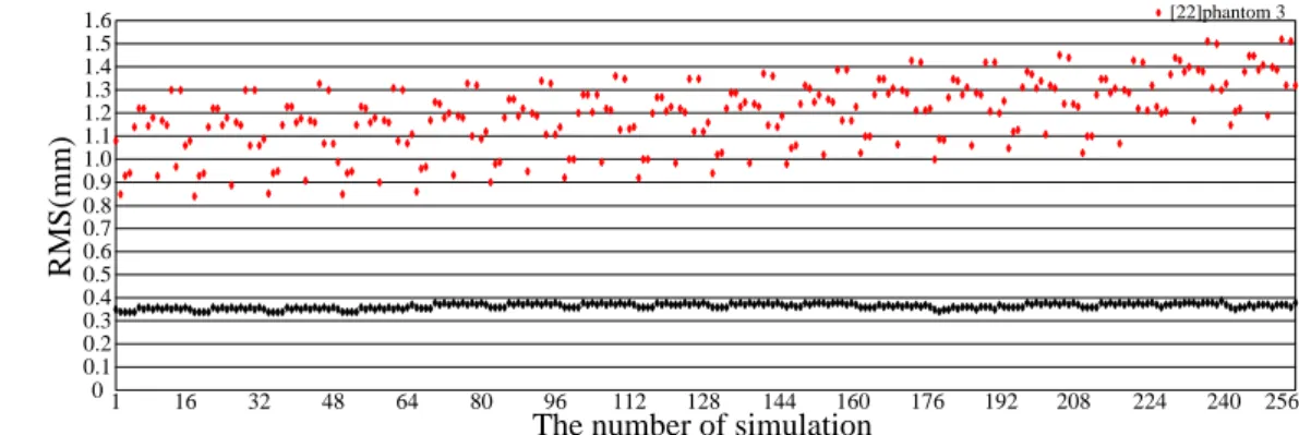
For this test, the same parameters are used for calculating results in Table 1, while the implanted and target points are changed. Specifically, the 16 implanted and target points are obtained from the meshesM1andM|B| respectively. In Figure 4, Experiment data show our RMS value is all less than 0.4 mm and have little change in the 256 simulation experiments. However, using the model of [22], the RMS values are higher and dynamic.

1.6 0.1 0.2 0.3 0.4 0.5 0.6 0.7 0.8 0.9 1.0 1.1 1.2 1.3 1.4 1.5 0 _{1 16 32 48 64 80 96 112 128 144} RMS(mm ) phantom 3 [22]phantom 3 160 176 192 208 224 240 256

The number of simulation

Fig. 4 RMS versus 256 test experiments for possible combinations of implanted and target points in phantom 3

3.5 Local performance comparison

To further evaluate the optimization strategy in Section 2.5, i.e., whether our method can well plan a surgical path at two ends of the guidewire, the same parameters are used for calculating results in Table 1, while the implanted point is changed. Figure 5 shows the effect by our optimization strategy for the phantom 1 and dataset 1 (first Rotterdam cardiac CTA dataset), where the virtual yellow-blue boxes shows the proposed method has a better local accuracy in comparing with the poor one in [22] and [23].

(b) (b1) (b2) (b3)

Fig. 5 Comparison of original guidewire and simulation ones on the phantom 1 and dataset 1. (a) and (b) are the original

guidewires, (a1) and (b1) are the simulated ones obtained by the method of [22], (a2) and (b2) are the simulated ones obtained by the method of [23], (a3) and (b3) are the simulated ones obtained by our method. The small pictures located in the virtual green or blue boxes show the enlarged curve segments, namely, the ones of interesting in each image with corresponding box color.

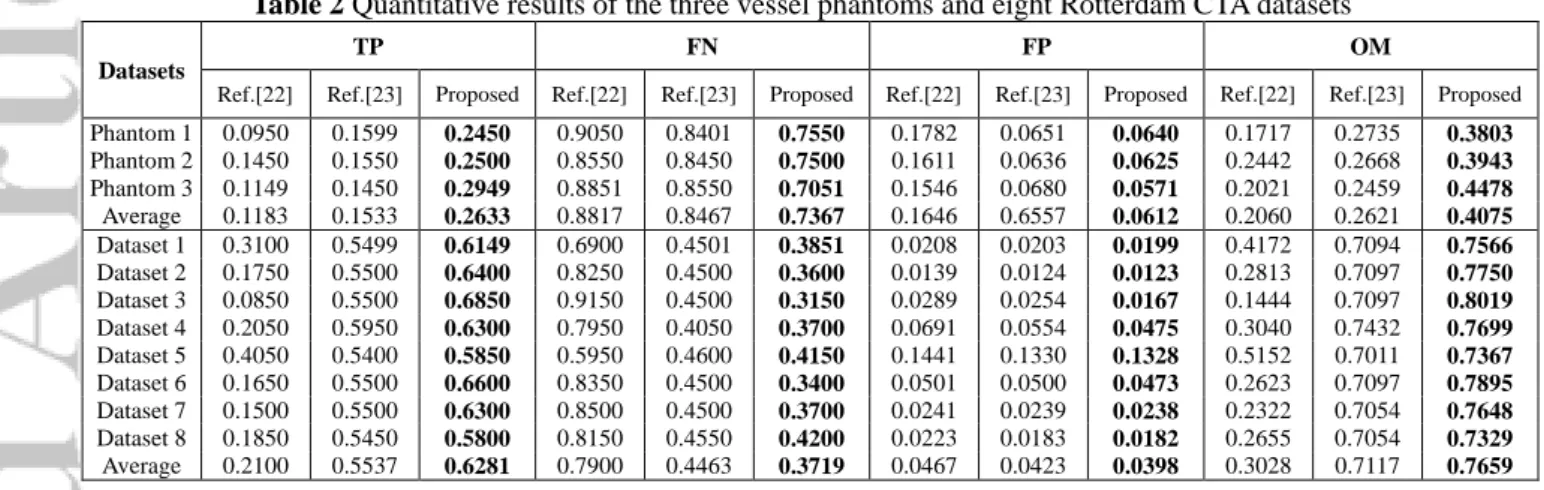
To further evaluate the local simulation accuracy, we manually divided each reference centerline into 10 parts, each part contains a 3D centerline with 20 points. The TP, FN, FP, and OM are then calculated in each part using (8). Finally, the average values of this four metrics are calculated, respectively. Table 2 shows TP, FN, FP, and OM, where the best results of this four metrics are shown in bold.

Table 2 Quantitative results of the three vessel phantoms and eight Rotterdam CTA datasets Datasets

TP FN FP OM

Ref.[22] Ref.[23] Proposed Ref.[22] Ref.[23] Proposed Ref.[22] Ref.[23] Proposed Ref.[22] Ref.[23] Proposed Phantom 1 0.0950 0.1599 0.2450 0.9050 0.8401 0.7550 0.1782 0.0651 0.0640 0.1717 0.2735 0.3803 Phantom 2 0.1450 0.1550 0.2500 0.8550 0.8450 0.7500 0.1611 0.0636 0.0625 0.2442 0.2668 0.3943 Phantom 3 0.1149 0.1450 0.2949 0.8851 0.8550 0.7051 0.1546 0.0680 0.0571 0.2021 0.2459 0.4478 Average 0.1183 0.1533 0.2633 0.8817 0.8467 0.7367 0.1646 0.6557 0.0612 0.2060 0.2621 0.4075 Dataset 1 0.3100 0.5499 0.6149 0.6900 0.4501 0.3851 0.0208 0.0203 0.0199 0.4172 0.7094 0.7566 Dataset 2 0.1750 0.5500 0.6400 0.8250 0.4500 0.3600 0.0139 0.0124 0.0123 0.2813 0.7097 0.7750 Dataset 3 0.0850 0.5500 0.6850 0.9150 0.4500 0.3150 0.0289 0.0254 0.0167 0.1444 0.7097 0.8019 Dataset 4 0.2050 0.5950 0.6300 0.7950 0.4050 0.3700 0.0691 0.0554 0.0475 0.3040 0.7432 0.7699 Dataset 5 0.4050 0.5400 0.5850 0.5950 0.4600 0.4150 0.1441 0.1330 0.1328 0.5152 0.7011 0.7367 Dataset 6 0.1650 0.5500 0.6600 0.8350 0.4500 0.3400 0.0501 0.0500 0.0473 0.2623 0.7097 0.7895 Dataset 7 0.1500 0.5500 0.6300 0.8500 0.4500 0.3700 0.0241 0.0239 0.0238 0.2322 0.7054 0.7648 Dataset 8 0.1850 0.5450 0.5800 0.8150 0.4550 0.4200 0.0223 0.0183 0.0182 0.2655 0.7054 0.7329 Average 0.2100 0.5537 0.6281 0.7900 0.4463 0.3719 0.0467 0.0423 0.0398 0.3028 0.7117 0.7659

3.6 Clinical metrics analysis

To further analyze the potential clinical application value of the proposed model, we consider the same parameters used for calculating results in Table 1 and then calculate the values of four metrics (OV, OF, OT, AI) respectively using (9). Finally, the average values of this four metrics are also calculated, respectively. Meanwhile, the best results are shown in bold. Due to OV, OF, OT, and their average value are all equal to 1 in [22], [23] and the proposed method, Table 3 only lists the AI metrics and AI average value, where the best results of this AI metrics are shown in bold. Although the metrics values of OV, OF, and OT are the same as [22] and [23], the proposed model has a minimum AI value and AI average value for the eight Rotterdam CTA datasets.

Table 3 Evaluation reports of the eight Rotterdam CTA datasets

Datasets Dataset 1 _(mm) Dataset 2 _(mm) Dataset 3 _(mm) Dataset 4 _(mm) Dataset 5 _(mm) Dataset 6 _(mm) Dataset 7 _(mm) Dataset 8 _(mm)

Averaged results of the eight datasets AI Ref.[22] 0.0332 0.0341 0.0322 0.0331 0.0331 0.0339 0.0321 0.0322 0.0330 Ref.[23] 0.0139 0.0137 0.0138 0.0138 0.0139 0.0138 0.0138 0.0138 0.0138 Proposed 0.0121 0.0125 0.0124 0.0124 0.0123 0.0123 0.0124 0.0126 0.0124 3.7 Running time

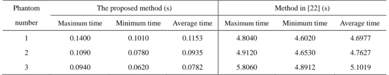
minimum running time, and average running time respectively for three phantoms. Statistical data are shown in Table 4. In addition, the system running time of proposed method is also shorter than that of [23] under the same conditions.

Table 4 system running times for three phantoms

Phantom number

The proposed method (s) Method in [22] (s)

Maximum time Minimum time Average time Maximum time Minimum time Average time 1 0.1400 0.1010 0.1153 4.8040 4.6020 4.6977 2 0.1090 0.0780 0.0935 4.9120 4.6530 4.7627 3 0.0940 0.0620 0.0782 5.8060 4.8912 5.1019

4 Discussion

In this study, we present a new matrix-based method to simulate the guidewire behavior inside an arterial system. Compared with previous method [22], our method improves previous iterative refinement procedure (i.e., cancel the parameter

α

and adopt an adaptive sampling strategy), and adopts the fusiform ternary tree approach as well as an optimization strategy based on proximal end and distal end of the guidewire. Meanwhile, a multi-thread technique is used to speed up aforementioned process. The experimental results show our method is more accurate and computationally more efficient than the existing method of [22].

The statistical data collected in Section 3.2 using different values of

δ

show that the range of the RMS value obtained by the proposed method is no more than 0.0939 mm and 0.0634 mm for phantoms 1 and 3, respectively. Whereas the range obtained by the method of [22] is no more than 0.9703 mm for phantom 1 and 0.5898 mm for phantom 3. Besides, the range of the RMS values obtained by the proposed method is no more than 0.0770 mm for phantom 2, while the range obtained by the method of [22] is no more than 0.7852 mm for phantom 2. Therefore, the proposed method is little influenced by parameter

δ

selection.

The statistical data collected in Section 3.3 using different numbers of sample points show that the RMS value obtained by the proposed method is a constant 0.3070 for phantom 3 (i.e., our method is insensitive to the number of sample points), whereas the range of the RMS value obtained by the method of [22] is 1.0347 mm for phantom 3. Besides, the RMS values obtained by the proposed method are still a constant for phantoms 1 and 2 respectively, while the range of the RMS values obtained by the method of [22] are 0.7581 mm and 0.8863 for phantoms 1 and 2, respectively. These results imply that the proposed method has a better robustness, i.e., it is insensitive to the number of sampled points, while the model of [22] can perform poorly when different numbers of sample points are used.

The study on the implanted point and target point in Section 3.4 (Figure 4) shows the range of the RMS values is 0.0387 mm by the proposed method. However, it is 0.6772 mm for phantom 3, under the method of [22]. Regarding the position modification of implanted point and target point, analogous comparison results can also be observed for phantoms 1 and 2. Hence, the proposed method has a better robustness on the location and direction of the implanted and target points.

The study on the implanted point in Section 3.5 (Figure 5) shows our optimization strategy given in Section 2.5 is more robust with better local accuracy. Under our optimization strategy, similar comparison results are obtained for phantoms 1 and 2, and the remaining seven Rotterdam datasets. The statistical data collected in Section 3.3 (Table 2) using TP, FN, FP and OM show our method has a better local simulation accuracy than that of [22] and [23] for three phantoms and eight Rotterdam datasets. Hence, the proposed method has a better robustness on the local performance for guidewire and its two ends.

The statistical data collected in Section 3.6 using OV, OF, OT, and AI (see Table 3) show that the metric AI value and AI average value obtained by the proposed model is smaller than that by the models of [22] and [23] for eight Rotterdam datasets. Therefore, the proposed method has a better clinical application potential.

5 Conclusion and future work

In this paper, a new matrix-based method has been presented to determine the guidewire position used in surgical operations. The proposed method improves the iterative refinement procedure of the existing method [22] and [23], and adopts the adaptive sampling strategy. The optimal path is obtained based on the fusiform ternary tree method and an optimization strategy with multi-thread technique. The empirical studies using three phantoms and eight Rotterdam

datasets reveal the proposed method has higher accuracy and more efficiency than the existing methods of [22] and [23]. We are interested in incorporating the physical properties of the guidewire into the proposed model for future work. Acknowledgements This work was supported in part by the National Key R&D Program of China (2018YFA0704102, 2017YFA0104302, Grant 2017YFC0109202 and 2017YFC0107900), in part by the National Natural Science Foundation (81827805, 61801003, 61871117), in part by the Fundamental Research Funds for the Central Universities, and in part by the Joint Research Project of Southeast University and Nanjing Medical University, in part by the technical product research project of Joint logistic support force of Chinese PLA (No. CLB18C050), and in part by the R&D Projects in Key Technology Areas of Guangdong Province (No. 2018B030333001).

References

1. Alderliesten T, Bosman PA, and Niessen WJ (2007) Towards a real-time minimally-invasive vascular intervention simulation system. IEEE Trans Med Imaging 26(1):128-132.

2. Alderliesten T, Konings MK, and Niessen WJ (2004) Simulation of minimally invasive vascular interventions for training purposes. Comput Aided Surg 9(1-2):3-15.

3. Alderliesten T, Konings MK, and Niessen WJ (2007) Modeling friction, intrinsic curvature, and rotation of guide wires for simulation of minimally invasive vascular interventions. IEEE Trans Biomed Eng 54:29-38.

4. A. Zijdenbos, B. Dawant, R. Margolin, A. Palmer (1994) Morphometric analysis of white matter lesions in MR images: Methods and validation. IEEE Transactions Image Processing 13(4): 716-724.

5. Bloom A, Gordon R, Vascular interventional radiology. Smith's general urology, 112, 2004.

6. Cai Y, Chui C, Ye X, Wang Y, and Anderson JH (2003) VR simulated training for less invasive vascular intervention. Comput Graph 27:215-221. 7. Cotin S, Duriez C, Lenoir J, Neumann P, Dawson S. 2005. New approaches to catheter navigation for interventional radiology simulation. In: Proceedings of medical image computing and computer-assisted intervention. 2005 Oct 26-30, Palm Springs (USA), MICCAI; p. 534-542.

8. Dawson SL, Cotin S, Meglan D, Shaffer DW, and Ferrell MA (2000) Designing a Computer-Based Simulator for Interventional Cardiology Training. Catheter Cardiovasc 51(4):522-527.

9. Euler L and Carathéodory C (1952) Methodus inveniendi lineas curvas maximi minimive proprietate gaudentes sive solution problematis isoperimetrici latissimo sensu accepti. Bousquet, Lausannae et Genevae, E65A. O.O. SER. I, Vol 24, 1744.

10. Fernando M. Cardoso, and Sergio S. Furuie. 2016. Guidewire path determination for intravascular applications. Computer Methods in Biomechanics and Biomedical Engineering. 19, 6 (2016), 628-638.

11. Hoda Sharei, Tanja Alderliesten, John J. van den Dobbelsteen, Jenny Dankelman. 2018. Navigation of guidewires and catheters in the body during intervention procedures: a review of computer-based models. Journal of Medical Imaging. 5, 1 (2018), 010902-1-010902-8.

12. J. Thorpe, Elementary Topic in Differential Geometry, Springer-Verlag, 1979.

13. Konings M, Van de Kraats E, Alderliesten T, and Niessen W (2003) Analytical guide wire motion algorithm for simulation of endovascular interventions. Med Biol Eng Comput 41(6):689-700.

14. Liu J, Hu Y, Yang J, Chen Y, Shu HZ, Luo LM, Feng QJ, Gui ZG, Coatrieux G (2018) 3D Feature Constrained Reconstruction for Low Dose CT Imaging. IEEE Transactions on Circuits and Systems for Video Technology 28(5): 1232-1247.

15. Liu J, Ma JH, Zhang Y, Chen Y (2017) Discriminative Feature Representation to Improve Projection Data Inconsistency for Low Dose CT Imaging. IEEE Transactions on Medical Imaging 36(12): 2499-2509.

16. Lenoir J, Cotin S, Duriez C, Neumann P. 2006. Interactive physically-based simulation of catheter and guidewire. Comput Graph. 30(3):416-422. 17. Landwehr P, Schindler R, Heinrich U, Dölken W, Krahe T, and Lackner K (1991) Quantification of vascular stenosis with color Doppler flow imaging: in vitro investigations. Radiology 178:701-704.

18. Luo MS, Xie HZ, Xie L, Cai P, Gu LX (2014) A robust and real-time vascular intervention simulation based on Kirchhoff elastic rod. Computerized Medical Imaging and Graphics. 38(8): 735-743.

19. Michiel Schaap, Coert T. Metz, Theo van Walsum, Alina G. van der Giessen, Annick C. Weustink (2009) Standardized evaluation methodology and reference database for evaluating coronary artery centerline extraction algorithms. Medical Image Analysis 13(5): 701-714.

20. Nowinski WL and Chui C-K (2001) Simulation of interventional neuroradiology procedures. Medical Imaging and Augmented Reality, 2001. Proceedings. International Workshop on, pp 87-94.

21. Przemyslaw Korzeniowski, Ruth J. White, Fernando Bello (2018) VCSim3: a VR simulator for cardiovascular interventions. International Journal of Computer Assisted Radiology and Surgery. 13(1): 135-149.

22. Qiu JP, Qu ZY, Qiu HQ, Zhang XM (2016) An improved real-time endovascular guidewire position simulation using shortest path algorithm. Med Biol Eng Comput 54(9):1375-1382.

23. Qiu JP, Zhang LB, Yang GY, Chen Y, Zhou SJ (2019) An improved real-time endovascular guidewire position simulation using activity on edge network. IEEE Access 6(7): 126618-126624.

24. Shen H, Wang C, Xie L, Zhou SJ, Gu LX, Xie HZ (2019) A novel robotic system for vascular intervention: principles, performances, and applications. International Journal of Computer Assisted Radiology and Surgery 14(4): 671–683.

25. Shen H, Wang C, Xie L, Zhou SJ (2018) A novel remote-controlled robotic system for cerebrovascular intervention [J]. The International Journal of Medical Robotics and Computer Assisted Surgery 14(6): 1943-1951.

26. Schafer S, Singh V, Hoffmann KR, Noël PB, and Xu J (2007) Planning image-guided endovascular interventions: guidewire simulation using shortest path algorithms. In: Medical Imaging, vol 6509, pp 65092C-1-65092C-10.

27. Schafer S, Singh V, Noël PB, Walczak AM, Xu J, and Hoffmann KR (2009) Real-time endovascular guidewire position simulation using shortest path algorithms. Int J Comput Assist Radiol Surg 4(6):597-608.

28. Shoujun Zhou, Baolin Li, Yuanquan Wang, Cheng Wang, Tiexiang Wen, Na Li (2018) The line- and block-like structures extraction via ingenious snake. Pattern Recognition Letters 112 (9): 324-331.

30. Wang YP, Chui CK, Cai YY, and Mak KH (1997) Topology sorted finite element method analysis of catheter/guidewire navigation in reconstructed coronary arteries. Comput Cardiol 24:529–532.

31. Xu J, Xu L, and Xie Y, (2010) Approximating minimum bending energy path in a simple corridor. In: Cheong O, Chwa K-Y, Park K(eds) Algorithms and Computation, vol 6506. Spring Berlin, Heidelberg, pp 328-339.

32. Xu L, Tian Y, Jin X, Chen J, Schafer S, Hoffmann K, and Xu J (2012) An improved endovascular guidewire position simulation algorithm. 9th IEEE International Symposium on Biomedical Imaging, pp 1196-1199.

33. Yu T and Zhang L (1996) Plastic bending: theory and applications. World Scientific, Singapore, pp 541-566.

34. Yang Chen, Jian Yang, Yudong Zhang, Huazhong Shu, Limin Luo, Coatrieux Jean-Louis Qjianjing Feng (2018) Structure-adaptive Fuzzy Estimation for Random-Valued Impulse Noise Suppression. IEEE Transactions on Circuits and Systems for Video Technology 28(2): 414-427.

35. Yang Chen, Yudong Zhang, Jian Yang, Qing Cao, Guanyu Yang, Jian Chen, Huazhong Shu, Limin Luo, Jean-Louis Coatrieux, Qianjian Feng (2016) Curve-like Structure Extraction Using Minimal Path Propagation with Backtracking. IEEE Transactions on Image Processing 25(2): 988-1003. 36. Zienkewickz O, Taylor R. The Finite Element Method. New York: McGraw-Hill, 1987.

Jianpeng Qiu received the M.S. degree from Lanzhou University in 2016. He is currently a doctor

student studying biomedical engineering at Southeast University. His research interests include biomedical engineering, multimedia information processing, and medical image processing.

Jian Yang received the Ph.D. degree in optical engineering from the Beijing Institute of

Technology in 2007. He is currently a Professor with the School of Optics and Photonics, Beijing Institute of Technology, Beijing, China. His research interests include medical image processing, augmented reality, and machine learning.

Yang Chen received the M.S. and Ph.D. degrees in biomedical engineering from First Military

Medical University, China, in 2004 and 2007, respectively. Since 2008, he has been a Faculty Member with the Department of Computer Science and Engineering, Southeast University, China. His recent work concentrates on the medical image reconstruction, image analysis, pattern recognition, and computerized-aid diagnosis.

Shoujun Zhou received the M.S. and Ph.D. degrees in school of information in Lanzhou University and biomedical engineering from First Military Medical University, China, in 2001 and 2004, respectively. Since 2010, he has been a Faculty Member with the Shenzhen institutes of advanced technology, Chinese academy of sciences, China. His recent work concentrates on the medical image analysis, pattern recognition, and computerized-aid diagnosis and therapy.

Liudong Xing received her Ph.D. degree in electrical engineering from the University of Virginia in 2002. She is currently

a professor with the Department of Electrical and Computer Engineering, University of Massachusetts (UMass) Dartmouth, USA. Her current research interests include reliability modeling, analysis and optimization of complex systems and networks. She is an Associate Editor or Editorial Board member of multiple journals including Reliability Engineering &