Calibration, feature extraction and classification of water contaminants using a differential mobility spectrometer

Calibration, Feature Extraction and Classification

of Water Contaminants Using a Differential

Mobility Spectrometer

by

Bobby Ren

Submitted to the Department of Electrical Engineering and Computer

Science

in partial fulfillment of the requirements for the degree of

Master of Engineering in Electrical Engineering and Computer Science

at the

MASSACHUSETTS INSTITUTE OF TECHNOLOGY

May 2006

@

Bobby Ren, MMVI. All rights reserved.

The author hereby grants to MIT permission to reproduce and

distribute publicly paper and electronic copies of this thesis document

MASSACHUSETTS INSTIFTE

in whole or in part. OF TECHNOLOGY

JUL 2 0

2009

LIBRARIES

A uthor

...

Department of Electrical Engineering and Computer Science

'

/ May 26, 2006

C ertified by

...

...

Nirmal Keshava

Head of Technical Staff

Thesis Supervisor

Certified by..

Dennis Freeman

Associate Professor

.- Thesis Supervisor

Accepted by

...

Arthur C. Smith

Chairman, Department Committee on Graduate Students

Calibration, Feature Extraction and Classification of Water

Contaminants Using a Differential Mobility Spectrometer

by

Bobby Ren

Submitted to the Department of Electrical Engineering and Computer Science on May 26, 2006, in partial fulfillment of the

requirements for the degree of

Master of Engineering in Electrical Engineering and Computer Science

Abstract

High-Field Asymmetric Waveform Ion Mobility Spectrometry (FAIMS) is a chemical sensor that separates ions in the gaseous phase based on their mobility in high electric fields. A threefold approach was developed for both chemical type classification and concentration classification of water contaminants for FAIMS signals. The three steps in this approach are calibration, feature extraction, and classification. Calibration was carried out to remove baseline fluctation and other variations in FAIMS data sets. Four feature extraction algorithms were used to extract subsets of the signal that had high separation potential between two classes of signals. Finally, support vector machines were used for binary classification. The success of classification was measured both by using separability metrics to evaluate the separability of extracted features, and by the percent of correct classification (Pcc) in each task.

Thesis Supervisor: Nirmal Keshava Title: Head of Technical Staff Thesis Supervisor: Dennis Freeman Title: Associate Professor

Acknowledgments

I would like to thank Nirmal Keshava, my Draper Advisor, for his guidance in the research and feedback on the manuscript, and Heidi Perry for her support. I would

like to acknowledge the members of the Bioengineering Group at Draper, including Melissa Krebs and Angela Zapata, for technical insights into FAIMS and help with data collection. Also, thanks to Dennis Freeman, my MIT Faculty Advisor, for giving feedback on the manuscript.

Contents

3 FAIMS Overview and Data Collection 19 3.1 Apparatus Setup . .... ... ... . . 20

3.2 Data Collection ... .... ... . 22

3.2.1 Acquisition . ... . 22

3.2.2 Chemical Basis ... ... 23

4 Methodology 25 4.0.3 Two Classification Tasks ... .... . . . 25

4.1 Step 1: Calibration ... ... . . 27

4.1.1 Preprocessing ... ... ... . . . . 27

4.1.2 Calibration ... ... . 29

4.1.3 Alternative Calibration Techniques ... .. ... . . . . 31

4.2 Step 2: Feature Extraction ... .. . 32

4.2.1 Pixel Domain vs. Wavelet Transform . ... 32 7

4.2.2 4.2.3 4.2.4 4.3 Step 3 4.3.1 4.3.2 4.3.3 4.3.4 Feature Prescreening . . . . Feature Extraction Algorithms . Quantifying Degree of Separation

Classification . ... Motivation ...

Classifier Formulation . . . . Kernel Selection . ...

Evaluation of Classification . . . 5 Results and Discussion

5.1 Calibration ...

5.2 Classification Results . . . .. 5.2.1 Classification Tasks . . . . . 5.3 Feature Set Score Metrics . . . . . 5.3.1 Normalized Univariate Class 5.3.2 SVM Margin Score . . . . . .. . . 34 .. . . . . . . . 35 . . . . . . . . . 4 0 .. . . . . 41 .. . . . 42 .. . . . 42 .. . . 44 .. . . . . . . 45 47 .. . . . . . 47 .. . . . 53 .. . . . . 55 .. . . . 69 Separability . ... 69 .. . . . . 71 6 Conclusion 6.1 Summary A Pcc Results

List of Figures

3-1 Ion movement due to asymmetric field mobility. . ... . 21

3-2 Unprocessed FAIMS signal. ... .... . 22

4-1 Removal of nitrogen and ammonium artifacts in FAIMS signals. . . . 28

4-2 Marginal FAIMS spectra before calibration. . ... 29

4-3 Boxplot of FAIMS intensities before calibration. . ... 30

4-4 Features measured for background intensity in boxplot. . ... 30

4-5 Peak to noise ratio for benzene 250ppm runs before baseline calibration. 30 4-6 The Haar mother wavelet. ... ... 33

4-7 Coefficients from 2-level wavelet decomposition. . ... 34

4-8 Wrapper feature extraction vs. filter feature extraction ... 36

4-9 SVM Mapping to a higher dimension . ... 45

4-10 k-Nearest Neighbors in 2-D space, k=3 . ... 46

5-1 Mean FAIMS Spectrum for benzene 125ppm. . ... 48

5-2 Mean FAIMS Spectrum for benzene 250ppm. . ... 48

5-3 Mean FAIMS Spectrum for benzene 500ppm. . ... . . 49

5-4 Mean FAIMS Spectrum for DCM 125ppm. . ... 49

5-5 Mean FAIMS Spectrum for DCM 250ppm. . ... 50

5-6 Mean FAIMS Spectrum for DCM 500ppm. . ... 50

5-7 Mean FAIMS Spectrum for water. ... . . . 51

5-8 Benzene 125ppm and 500ppm signal comparison. . ... . . 51

5-9 Marginal FAIMS spectra before and after calibration. . ... 52

5-11 Peak to variance ratio in benzene 250ppm before and after calibration. 53

5-12 Pcc for benzene 250ppm vs DCM 250ppm in the pixel domain. ... 55

5-13 Pcc for benzene 500ppm vs DCM 500ppm in the pixel domain. ... 57

5-14 Features selected for benzene 250ppm and DCM 250ppm in the pixel domain. ... ... ... ... 58

5-15 Features selected for benzene 500ppm and DCM 500ppm in the pixel domain . ... 59

5-16 Pcc for benzene 125ppm vs benzene 500ppm in the pixel domain. . . 60

5-17 Features selected for benzene 125ppm and benzene 500ppm in the pixel dom ain. .. . . ... .. . . . ... . . . ... .. . . . . .. 61

5-18 Pcc for DCM 250ppm vs DCM 500ppm in the pixel domain. ... 62

5-19 Features selected for DCM 250ppm and DCM 500ppm in the pixel domain . ... .... ... 63

5-20 Pcc for benzene 125ppm vs DCM 125ppm in the wavelet domain. .. 64

5-21 Reconstruction of benzene 125ppm and DCM 125ppm with wavelet features . . . . . ... . . 65

5-22 Pcc for DCM 125ppm vs DCM 500ppm in the wavelet domain. . . . 66

5-23 Reconstruction of DCM 125ppm and DCM 500ppm with wavelet fea-tures selected by RFS. ... ... ... 67

5-24 Mean FAIMS Spectrum for DCM 500ppm . ... 68

5-25 NUCS score vs Pcc for all feature sets in the pixel domain... . 70

5-26 NUCS score vs Pcc for all feature sets in the wavelet domain .... 70

5-27 SVM margin vs Pcc for all feature sets in the pixel domain. ... 71

5-28 SVM margin vs Pcc for all feature sets in the wavelet domain. .... 71

A-1 Pcc for benzene 125ppm dcm 125ppm, pixel domain. . ... 78

A-2 Pcc for benzene 250ppm dcm 250ppm, pixel domain. . ... 78

A-3 Pcc for benzene 500ppm dcm 500ppm, pixel domain. ... 79

A-4 Pcc for benzene 125ppm benzene 250ppm, pixel domain. ... . 79

A-6 Pcc for benzene 250ppm benzene 500ppm, pixel domain. ... 80

A-7 Pcc for dcm 125ppm dcm 250ppm, pixel domain. . ... . . 81

A-8 Pcc for dcm 125ppm dcm 500ppm, pixel domain. . ... . . 81

A-9 Pcc for dcm 250ppm dcm 500ppm, pixel domain. . ... . . 82

A-10 Pcc for benzene 125ppm dcm 125ppm, wavelet domain. ... 82

A-11 Pcc for benzene 250ppm dcm 250ppm, wavelet domain ... 83

A-12 Pcc for benzene 500ppm dcm 500ppm, wavelet domain ... .. 83

A-13 Pcc for benzene 125ppm benzene 250ppm, wavelet domain. ... 84

A-14 Pcc for benzene 125ppm benzene 500ppm, wavelet domain. ... 84

A-15 Pcc for benzene 250ppm benzene 500ppm, wavelet domain. ... 85

A-16 Pcc for dcm 125ppm dcm 250ppm, wavelet domain. . ... . 85

A-17 Pcc for dcm 125ppm dcm 500ppm, wavelet domain. . ... . 86

List of Tables

3.1 Benzene and Dichloromethane. ... .. 23

3.2 Available data samples by class ... .. 23

5.1 Classification tasks performed. ... ... 54

5.2 Feature scores for benzene 250ppm vs. DCM 250ppm, pixel domain . 56 5.3 Feature scores for benzene 500ppm vs. DCM 500ppm, pixel domain . 56 5.4 Feature scores for benzene 125ppm vs. benzene 500ppm, pixel domain 61 5.5 Feature scores for DCM 250ppm vs. DCM 500ppm, pixel domain . . 61 5.6 Feature scores for benzene 125ppm vs. DCM 125ppm, wavelet domain 66 5.7 Feature scores for DCM 125ppm vs. DCM 500ppm, wavelet domain . 68

Chapter 1

Introduction

1.1

Motivation

High-Field Asymmetric Waveform Ion Mobility Spectrometry (FAIMS) is a recently developed differential mobility spectrometer that separates ions in the gaseous phase based on their mobility in high electric fields. Traditional ion mobility spectrometry (IMS) is useful for separating ions based on size-to-charge at low field strengths. However, at low field strengths, ion mobility does not serve as a highly differentiating characteristic, whereas at high field conditions ion mobility can be used to characterize different chemicals[17]. Typical mass spectrometers, are also expensive and relatively large, and require operation at low pressures that cannot be easily reproduced in the field[10]. FAIMS, which operates at atmospheric pressure, is designed to separate ions based on differences in ion mobility in a high asymmetric radio-frequency electric field. With the right algorithms and software techniques, it is a tool that may pave the way for handheld tools that can be used in a wide variety of clinical and environmental applications.

1.2

Previous Work

Much previous work has been done to explore the utility of FAIMS. FAIMS was first developed at the Charles Stark Draper Laboratories in 1998 as a smaller, portable

tool for mass spectroscopy without compromising sensitivity or performance [6]. It has since been used in many applications, ranging from monitoring water quality to classifying potential biological weapons for homeland security[10]. This thesis is a logical extension of previous work of applying statistical algorithms toward the detection of impurities in water[3]. We emphasize classification between different contaminants rather than detection of a single contaminant in an otherwise clean background.

1.3

Project Goal

The goal of this thesis is the classification of FAIMS spectra involving two chemicals, benzene and dichloromethane. A three step algorithm will be developed: calibration, feature extraction, and classification. Calibration is a preanalysis step necessary because of observations of sensor drift. Feature extraction, on both pixel intensities and wavelet transform coefficients, will involve filter and wrapper methods to capture the most distinguishing features from the FAIMS spectra. Finally, classification will be performed with support vector machines (SVMs), a popular classification technique for bioinformatics. We also prefer SVMs because it is nonparametric and thus does not require class statistics to be effective. This threefold approach for classifying simple compounds may one day be extended to solving more complex classification problems with the FAIMS apparatus.

Chapter 2

Project Overview

2.1

Motivation

The FAIMS sensor is an alternative tool to traditional mass spectroscopy, and has potential for field and clinical applications because of its size and low cost. However, techniques for field applications of FAIMS sensors are not perfect. Furthermore, sensor drift and other variations of the instrument over time can make the FAIMS output difficult to interpret. We seek a method to extract reliable features from FAIMS spectra for classification that will still be robust to day to day changes in instrument sensitivity and field conditions.

The development of a general algorithm for performing classification with FAIMS data involves a threefold approach: calibration, feature extraction, and classifica-tion. This research will focus on the development of such a method for classifying between two chemical contaminants, benzene and dichloromethane. The process may be extended for other pairs of chemicals, and may be adapted to a large range of applications in the field.

2.2

Threefold Approach

First, the collection and processing of raw FAIMS data involves an investigation into calibration methods for the FAIMS sensor. The goal of calibration is to prepare

raw FAIMS data for the classification process by removing artifacts resulting from sensor drift, excessive noise, and FAIMS operational noise that may negatively affect the training of a robust classifier. There have been no literature on calibrating the

FAIMS sensor for classifying chemicals, but initial experiments show that calibration is needed in order to accurately train classifiers.

Second, feature extraction using various algorithms is applied to extract features that can be submitted to a classifier. These features should be robust subsets of the spectra that distinguish between two classes of signals. We will explore both filter and wrapper algorithms. Filter algorithms produce features that have no specificity to a particular classification technique, whereas wrapper algorithms use the results of classification algorithm to improve on the feature selection process. Features will either come from raw pixel data of the FAIMS spectra or from wavelet coefficients (the transform domain). Thus, feature extraction will also involve exploring the wavelet decomposition of FAIMS data and how that contributes to the feature set.

The third step of the threefold approach is to be able to classify contaminants using FAIMS spectra. We focus on support vector machine classification between two chemical contaminants. SVMs are a popular classification tool in the bioinfor-matics field and have been used at Draper Labs to classify stem cell images[8]. This nonparametric approach allows for flexibility of input data; SVMs do not assume specific distribution of data, and are also powerful in dealing with both linearly and nonlinea.rly separable data.

Finally, the performance of the three step algorithm will be measured by its per-centage of correct classification (Pcc). The Pcc is the perper-centage of a test data set that is correctly classified by the SVM classifier. The effectiveness of the feature extraction algorithms will also be evaluated using various measures of distance.

Chapter 3

FAIMS Overview and Data

Collection

FAIMS first emerged in the 1990s as a new tool for mass spectrometry. It is a relatively new development in a field that has sought instruments capable of sep-arating compounds into their components based on chemical properties. In classic mass spectrometry, a mass spectrometer is coupled with gas chromatography to pro-duce chemical fingerprints for compounds that can be matched in a library. In the search for better mass spectrometry instruments, ion mobility spectrometry (IMS) was developed in the 1970s by combining radioactive ionization with drift tube ion separation[18]. Successful applications of IMS include hand held chemical agent mon-itors (CAM) used for detection of chemical warfare agents[13].

However, at low field strengths, ion mobility does not serve as a highly differ-entiating characteristic, whereas at high field conditions ion mobility can be used to characterize different chemicals. Typical mass spectrometers are also expensive and relatively large, and require operation at low pressures that cannot be easily re-produced in the field. Extensions of IMS include the addition of high electric fields produced between two parallel plates[2]. A cylindrical configuration, named the Field Ion Spectrometer (FIS), was introduced by the Mine Safety Appliances Company[6]. Finally, in 1998 the FIS was combined with a mass spectrometer, capable of atmo-spheric ion separation[17], and became the FAIMS. FAIMS has the advantages of

being more portable, inexpensive and faster in operation than traditional tools of mass spectrometry.

Miniaturization of IMS has been a long time goal in the mass spectrometry field be-cause of the potential to develop handheld, field-applicable tools. In 1998 researchers at Draper studied FAIMS, also called the differential mobility spectrometer, as a portable tool for chemical detection, and developed a micromachined (MEMS) ver-sion of the parallel plate FAIMS[13, 14]. This miniaturized technology is currently being used in the Draper laboratory for a wide variety of applications. Using pyrolysis to prepare and introduce biological agents, signature biomarkers for chemical weapon agents such as anthrax spores were studied[10]. To facilitate FAIMS applications in the field, methods for statistical detection of contaminants using FAIMS outputs were explored in 2005[3].

3.1

Apparatus Setup

The FAIMS apparatus at Draper Labs used in this research consists of headspace sampling, gas-chromatography, ionization with Ni-63, and a MEMS differential mo-bility sensor (DMS), which is capable of detection at the part-per-trillion scale[10].

First, a sample of water with contaminants is heated and vapor from the headspace of each sample is injected into the gas chromatography column. Temporal separation results from how long the chemical sample takes, relative to water vapor that enters with the chemical, to pass through the column.

Analytes exiting the column are ionized by a radioactive nickel source before entering the DMS, where a pair of parallel plates apply an asymmetric waveform of alternating high and low electric fields perpendicular to the flow of the carrier gas. This field causes the analyte ions to drift perpendicular to the direction of the carrier gas.

As seen in Figure 3-1, the electric field is applied with an asymmetric high and low waveform. The net electric field over time is zero. An ion's mobility can be approximated by K(E) = K0(1 + a(E)) where K0 equals the low field mobility[14].

Caniergas

AY

direction

1E

Fl. F -.. time

Figure 3-1:. Ion movement due to asymmetric field mobility.

When E is large, the ion mobility will change depending on the factor a(s). Because of this unequal mobility in the alternating high and low electric fields, an ion will have a nonzero net drift toward one of the plates. Its movement in the direction of the electric field is AY = K(E)Et. Because Eltlo = Ehithi, the amount of drift depends

on the low and high field mobilities for that ion. Figure 3-1 shows the direction of drift for two ion species that have different mobilities.

For a certain average field strength, some compounds will flow right through the channel, while other compounds will be absorbed into the plates. By applying a range of compensation DC fields, all ions can be made to either drift through to the sensor or into the parallel plates. Thus, FAIMS is capable of detecting and visualizing, at high temporal and spatial resolutions, ion intensities for samples that may have very low chemical concentrations.

Figure 3-2 shows a sample FAIMS spectrum. Time is on the X axis, and t = 0 is located where the main cluster for the ammonium artifact ends. The 100 values of compensation voltage are on the Y axis. The figure shows a raw FAIMS sample before processing (see Section 4.1.1).

Benzene 125ppm before preprocessing 8 5 3 0 -2 -5 -7 P -10 -12 o -25 -27 -30 -32 -35 -37 -40 0 50 99 149 198 248 298 347 397 446 496 546 time (s)

Figure 3-2: Unprocessed FAIMS signal.

3.2

Data Collection

3.2.1

Acquisition

Data samples were gathered by Melissa Krebs of Draper Labs from November 3, 2005 through November 15, 2005. All samples were taken with the same machine parame-ters. The headspace sampler, where the vials of liquid are stored and sampled, is in an oven at 60 degrees C. Samples of headspace are injected into the gas chromatography oven at 40 degrees C and held at that temperature for 30 seconds. The oven is then ramped up to 100 degrees C at 10 degrees/minute. Nitrogen is used as the carrier gas, at 1.5 ml/min through the GC column, and 300 ml/min in the main FAIMS flow. Each run spanned 100 compensation voltage values that ranged from -40V to 10V, for approximately 500 scans over approximately 10 minutes. The radio frequency of the alternating field is 1200 Hz.

Chemical Benzene DCM H

Structure H

Molecular weight 78.1134 84.9328

Water solubility 0.18 g/100 mL 1.32 g/100 mL

EPA Maximum Contaminant Level 5 ppb 5 ppb

Table 3.1: Benzene and Dichloromethane.

Benzene _{DCM Water (control)}

125 ppm 99 100

250 ppm 101 100

500 ppm 100 100

-0 ppm (control) - - 30

Table 3.2: Available data samples by class

3.2.2

Chemical Basis

Benzene and dichloromethane (DCM) are government regulated solvents that have a health risk if found at high levels in drinking water[4, 5]. Table 3.1 shows the chemical structure and various characteristics about each chemical.

It was found empirically that the chemicals were difficult to detect below concen-trations of 50 ppm, and that 1000 ppm was too large to produce clean data. Thus, the three concentrations used were 125, 250, and 500 ppm for both chemicals. The data were gathered over a period of two weeks using the batch collection ability of the FAIMS setup. A total of 15 datasets were taken, with roughly 44 samples in each set consisting of about 21 benzene at various concentrations, 21 DCM at various concen-trations, and 2 of pure water. In each set, the order of chemicals and concentrations was randomized so that drift and machine error would not bias the data; see Section 4.1 for more insight into the effects of FAIMS sensor drift. After data collection, carried out by Krebs, the datasets were consolidated into 7 data sets, consisting of benzene at 125 ppm, 250 ppm, and 500 ppm, DCM at 125 ppm, 250 ppm, and 500 ppm, and water as a control. Table 3.2 shows the number of samples available in these sets.

Chapter 4

Methodology

4.0.3

Two Classification Tasks

In our threefold approach, we seek to develop a binary classifier that can classify two classes of FAIMS data. The data is composed of two chemicals at three different concentrations each. This creates two classification tasks that will be examined. In the first task, we are classifying two different chemical contaminants that are at the same concentration. In the second task, we classify two concentrations of the same contaminant. Thus, the two tasks are:

1. Chemical Classification: chemical A vs chemical B, both at concentration a. 2. Concentration Classification: chemical A at concentration a vs chemical A at

concentration 3p.

In developing a algorithm to classify between two classes of FAIMS data, we consider a signal model based around a binary hypothesis test:

H1 : r(Vc, t) = s (V,, t) + ni(V,, t) (4.1)

H2 : r(V, t) = S2(Vc, t) + n2 (V, t) (4.2)

In every classification task we assume that the output of the FAIMS sensor r (V, t) consists of the signal si(V, t) corresponding to a class of contaminant added to a

background of noise ni(V, t). This model can be further simplified by assuming that the noise is statistically identical in both cases, but this is not rigorously proven. Given a set of training samples, a classifier must be able to make a decision on whether an unknown test sample runknown fits hypothesis H1 or H2. The threefold

approach that has been developed for calibration contains the following three steps: 1. Calibration

2. Feature Extraction 3. Classification

Chemical Classification

First, we want to classify between the two types of chemical contaminants. The sup-port vector machine will be trained on a set of benzene at concentration a and a set of DCM at the same concentration a. The goal is to then be able to distinguish what type of chemical contaminant is in a sample of unknown chemical at that same concentration. We want to determine whether a classification algorithm can be de-veloped that will classify between the datasets, and whether concentration affects the ability to classify.

Classifying between benzene and DCM at the same concentration may be very straightforward. First, each contaminant is pure; both are single symmetricx molecules that do not have isomers -left or right handed configurations that can behave differ-ently. In biomarker detection, FAIMS inputs consist of more complex molecules and mixtures that produce multiple-peaked signatures[10]. Benzene and DCM should both only produce one peak each, and will be detected by the FAIMS at different temporal (t) or spatial (V) locations, thus their signature spectra s(V, t) should be easy to identify and distinguish.

Concentration classification

The second classification task we consider is to distinguish between samples of the same chemical contaminant at different concentrations. A set of samples at

con-centration a and a set of samples of the same chemical at concon-centration 3 will be used as training data for the concentration classifier. We want to determine whether it is possible to classify between the same chemical at different concentrations, and whether the type of chemical or the relative concentrations of that chemical affect classification outcome.

Despite being the same chemical, FAIMS spectra of two classes at different con-centrations may have features that are different in both temporal-spatial location and intensity. Depending on whether the FAIMS sensor responds linearly to concentra-tion, concentration classification may involve both intensity and location. There is evidence that the FAIMS output for many chemicals does not vary linearly over large ranges of concentration[3].

4.1

Step 1: Calibration

As with many sensor instruments, the sensitivity and response of the FAIMS sensor can vary with time. No literature was found to discuss calibration techniques for FAIMS applications. For FAIMS spectra, we consider three sources of variation:

1. Temporal variation 2. V or spatial variation

3. Intensity or baseline variation

In our analysis of experimental data, we observed that readings from a FAIMS measurement can fluctuate from day to day, or even over the course of an hour. Because the collection occurred over the course of about two weeks, with each batch collection taking several hours, sometimes overnight, it is necessary to address the variations in the raw data before doing any further analysis.

4.1.1

Preprocessing

Before any calibration, feature extraction, or any other analysis was performed, the data was processed to remove nonessential spectra. Due to the carrier gas, there

Benen 125ppm before poproc ng Benzene 125ppm after preprocessing s 6 0.7 3 4 o 2 40.6 -2 -s 0.5 -- 4 , -129 I 0.4 1s 11 0.3 -2 19 0.2 -2722 1 -21 2 0 -20.1 -27 -2 -30o -310 -32-34 S-3 .0.1 -37 -39 0 140 1e 248 20 347 44 40 50 90 149 198 248 298 347 397 448 496 546 tm. (a) time (s)

Figure 4-1: Removal of nitrogen and ammonium artifacts in FAIMS signals.

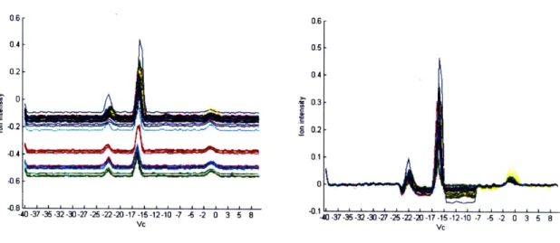
are several artifacts in the FAIMS spectra that would make feature extraction and calibration difficult. The nitrogen carrier gas produces a large, high intensity streak along the time axis at around compensation voltage Vc=-15V. The presence of this line can be used for spatial calibration by making sure it shows up in the same V position over all samples.

When the initial amount of water vapor emerges, the FAIMS signal will show an ammonium artifact in which the nitrogen line disappears and there is a "dip" at Vc=-21V. This dip is visually helpful in locating the start time of each sample, where t is set to 0. If locating the dip is accurate, using the ammonium artifact as a temporal reference point serves as a form of temporal calibration.

However, because the intensity of these two artifacts is so great, they are likely to completely outweigh any measured ion intensity from the contaminant. Thus, before calibration and feature extraction, the nitrogen line and ammonium dip are removed from the data. Figure 4-1 shows the spectra directly from the data, and after preprocessing, in which the signature of the measured chemical is much easier to see.

-02

840-37-35-32-30-27-25 -22- -17-15-12-10 -7 -5 -2 0 3 5 8 Vc

Figure 4-2: Marginals for benzene 250ppm before baseline calibration.

4.1.2

Calibration

Variation in baseline intensity occurs due to drift of baseline values in FAIMS sensi-tivity. In preliminary studies, test datasets that were taken on a different day than training sets of the same class were misinterpreted as a different class. Thus, this base-line fluctuation has a significant impact on the success of classification between classes and must be removed. Figure 4-2 shows fluctuation of baseline values throughout the collected data in the benzene 125ppm set as seen by the changes in their marginals. The marginal of a FAIMS sample is calculated by integrating the FAIMS signal over time (Eq. 4.3). Figure 4-3 shows a boxplot of the intensities of a small subset of

200 randomly chosen feature for each run in the benzene 125ppm dataset, in which samples 86-96 show significant differences in mean intensity. The features comprise mostly of background noise, as represented by the white pixels in Figure 4-4.

Rvc (Vc) =

Z

t

Another type of intensity variation is the change in signal to noise ratio (SNR). Baseline fluctuations do not simply add a constant value to the intensities in a signal. When the FAIMS sensitivity changes, it is possible that the strength of the measured signal changes, and thus the SNR will be different from sample to sample. This change may cause a classifier to wrongly distinguish subsets of data that belong to

1 6 11 16 21 26 31 36 41 46 51 56 61 Data run

66 71 76 81 86 91 96 101

Figure 4-3: Boxplot for benzene 250ppm intensities before baseline calibration.

14 1t time (s)

Figure 4-4: Features measured for background intensity in boxplot.

20 40 60

Data run

80 100 120

Figure 4-5: Peak to noise ratio for benzene 250ppm runs before baseline calibration.

0.2 0.1 0 I -0.3 --0.3 -06 ii ii 300 280 260 240 z 220 200 CL

the same class, simply because they have lower measured peaks. This effect can be seen in the difference between the size of the largest peaks in Figure 4-2. Since the nitrogen artifact should be independent of time and chemical type, the nitrogen peak

(Vc = -16V) should remain constant, but instead those runs with more negative

baseline values seem to have smaller nitrogen peaks. As seen in Figure 4-5, these smaller peaks result in a smaller signal to noise ratio. Calibration will also try to address the fluctuations in peak to noise ratio.

To calibrate all the data, the wavelet transform was used for baseline removal. The wavelet transform is capable of decomposing an image into approximation and detail levels at different scales. At a high scale (N=4), the approximation is close to the DC value, but may also include other low frequency artifacts. Thus wavelet calibration involves simply removing the level 4 approximation of each signal, and keeping the detail signal. Wavelets are discussed in more detail in Section 4.2.1.

Thus, in order to calibrate FAIMS, the following four steps are taken: 1. Temporal calibration in reference to ammonium dip

2. Spatial calibration in reference to nitrogen line 3. Removal of nitrogen and ammonium artifacts

4. Intensity calibration by wavelet transform baseline removal

4.1.3

Alternative Calibration Techniques

There are other possible calibration techniques that were not explored due to time constraints. There is an additional set of FAIMS spectra for diluted water with no chemical added. It is possible that these samples could have helped in determining some baseline level of noise for baseline calibration. However, this type of calibration reference may be more suitable for a detection algorithm in which there is need to quantify the background statistics.

The use of the ammonium dip as a temporal reference is not ideal, because the method of determining exactly when the dip starts and ends is not accurate. Dis-cussions at Draper brought up the use of an internal standard in the FAIMS. Such

standards would be well studied and known to be consistent in their emergence time. One such standard could be the chloride ion studied by Viehland, whose mobility was calculated using FAIMS to agree with well published drift tube mobility[19].

4.2

Step 2: Feature Extraction

Feature extraction seeks to isolate and extract features in FAIMS spectra for use in classification. A single FAIMS signal has up to 50,000 dimensions (500 temporal values, 100 Vc values). The goal of feature extraction is to reduce the dimensionality as much as possible while capturing as much of the discriminating features of the FAIMS signal as possible. This final feature set should create the largest "distance" possible between the two classes that are to be classified. There are several steps to feature extraction: wavelet domain transformation, filter prescreening, and finally, feature extraction in both the pixel and wavelet domains.

4.2.1

Pixel Domain vs. Wavelet Transform

The most important features in a set of data are not always obvious from the pixel representation. Single pixels are not adequate features if, for example, a chemical appears in the FAIMS spectrum over a large region, or if temporal variations remain after calibration. However, in the wavelet transform domain, it is possible to isolate and extract features that are larger than one pixel in size, and therefore more robust to system imperfections.

Wavelets[11] are compactly supported, time limited signals that can be dilated and translated to form a multiresolutional basis, which is then used to decompose the image in both the time and the frequency domains. The Haar wavelet, also known as the Daubechies wavelet dbl, is shown in Figure 4-6. It is a step function, the simplest of the mother wavelet functions[15].

Wavelet coefficients are produced by correlating the pixel image with scaled and translated versions of the mother wavelet:

I

t7777771-0 0.5 1

Figure 4-6: The Haar mother wavelet.

Wa,b = a2 ( (4.4)

Whereas in the pixel domain, features selected are single pixels with high differen-tiation potential, the wavelet transform coefficients correspond to areas of different sizes, matching up with the basis functions at different scales.

In image processing, the 2D discrete wavelet transform is used to filter an image both horizontally and vertically into an approximation signal A and three detail signals Dh, Dv and Dd. Dh corresponds to filtering for the high horizontal and low vertical frequencies of the image, Dv are the low horizontal and high vertical frequencies, and Dd are the high horizontal and vertical frequencies. In multiple level deconstructions, the approximation signal is then decomposed again to produce a smaller approximation signal and three corresponding detail signals. Figure 4-7 shows the pyramid structure of the deconstruction. The original image can be completely reconstructed using the highest level approximation plus every detail coefficient.

By using the wavelet transform to analyze the data, an alternate basis is provided from which to select features for classification. For each set of classification tasks, both pixel and wavelet data will be used for feature extraction and classification. Note that in this paper "data" and "features" will refer to either wavelet coefficients or pixel intensities if not specified, as an orthonormal wavelet decomposition yields the same number of transform domain coefficients as the pixel representation.

Dv

Ddl

Dv2

Dd2

Dhl

Dh2

Figure 4-7: Coefficients from 2-level wavelet decomposition.

4.2.2

Feature Prescreening

In both the pixel and wavelet domains, FAIMS spectra are still represented as 50,000 coefficients. We would like to screen out a large number of features that have no value for classification. If features that are unlikely to be distinguishing are first removed, the feature selection process will be much faster with little or no loss of performance. An initial stage of prescreening is done to select the top 1000 features that have the greatest distance between the two training classes and from which the final subset of features will be chosen. We use a simple metric for gauging the separability of two classes that is related to Fisher's Linear Discriminant (4.5):

S(_{PI - 22}

D(i)= (4.5)

We will refer to this separability measure as the normalized univariate class separabil-ity (NUCS). For the ith feature, pI1 and al are its mean and variance in class 1, and I2 and o2 are its mean and variance in class 2. This measure is applied to both the pixel

and wavelet coefficients and selects for features that have a large distance measure between the two classes. The remaining 1000 features provide a much smaller search space for the main feature extraction algorithms.

4.2.3

Feature Extraction Algorithms

Filters vs. Wrappers

Four feature extraction algorithms have been developed to extract features from train-ing data. In all feature selection algorithms, features are selected by evaluattrain-ing their effectiveness using various criterion functions. If the set of all features is X and the criterion function for a subset of features S is J(S), feature extraction algorithms will try to find the set S C X of length d to maximize its criterion value:

J(S) = maxsCx,tSl=dJ(S) (4.6)

The criterion used divides the algorithms into two classes: wrappers and filters. Wrap-pers are feature selection algorithms in which the induction algorithm, or the classifier, is used as part of the evaluation criterion for the features[9]. In training the classifier, the training data is divided into subsets that are used to crossvalidate the feature sets selected. The feature set with the highest classification score is selected. Filter algo-rithms, on the other hand, use a separability measure to select features independently of the classifier. They are independent of a specific classification algorithm and thus are very versatile, but wrappers can have better performance if they select features relevant to the classification algorithm[9]. Figure 4-8 shows the process in which features are extracted using a wrapper method, compared with the filter method.

The four feature extraction algorithms implemented are:

* Magnitude Signature

* Sequential Forward Selection (SFS)

* SVM-aided Recursive Feature Elimination (RFE) * SVM-aided Recursive Feature Selection (RFS)

The first feature extraction algorithm is a filter method called the magnitude signature filter. Its criterion function is simply the magnitude of the coefficients, and the largest coefficients are ranked higher. Sequential forward selection is a filter

Wrapper

Training

Classf er

Data

ection

coring

Filter

TrainingBest feature set

Training

Separability

Measure

Classifier

Data

Figure 4-8: Wrapper feature extraction vs. filter feature extraction.

method that was first proposed by Whitney [20]. We combine its forward selection algorithm with the divergence scoring metric (see Sec. 4.2.3). The last two methods, Recursive Feature Elimination and Recursive Feature Selection, are wrapper methods that use SVMs as the criterion. SVM-aided Recursive Feature Elimination (RFE), which eliminates the lowest ranked feature at each iteration has been used in gene expression feature selection[7]. SVM-aided Recursive Feature Selection (RFS) is a technique derived from RFE, and selects features in a forward manner similar to

SFS.

Magnitude Signature Filter

The magnitude signature feature extraction method assumes that in the absence of chemical contaminant, the noise signature consists of white noise of very low intensity. When a chemical contaminant does emerge, its signature can be identified by finding the features with the largest magnitude. However, the overall feature set of each training class X is selected among the sample runs x by finding the features that are selected the most often by each sample. For each class, half the total number of features are selected, then the features from both classes are combined. All features

are ranked individually, thus the criterion function (Eq. 4.8) is an individual score, and feature scores are not evaluated as a group.

For each data run, the top K features with the greatest squared magnitude are saved, represented by Features(X). Define a function SelectedBy(x) to equal 1 when a. feature i is one of the features selected by x:

Slt () 1 if i C Features(x)

SelectedBy(x) = - (4.7)

0 otherwise

To find the signature set for the class as a whole, the features are ranked by how many times they have been selected in that set, so the scoring function for each feature is:

J(i) = C SelectedBy(x) (4.8)

xCX

It follows that the higher the value of this criterion function, the more important the feature is for the set.

When selecting for N features to distinguish two classes, each class contributes half of the feature set, or N features. This way, features prominent in either class will be chosen as a distinguishing feature. It may be possible to adjust the number of features each class is allocated, if any knowledge exists about the density of features in each class. Other parameters that can be adjusted include the number K of top ranking features each run selects, which can affect the stringency of the feature selction process. In this thesis, K = 100. A lower number of features selected can result in a feature set that appeared in only a low percentage of runs, but a higher number may result in features that are not distinguishing being selected.

Sequential Forward Selection

The sequential forward selection algorithm (SFS), first put forward by Whitney in 1971, is a simple feature selection algorithm that uses the divergence criterion to score the effectiveness of a feature set. Divergence (Eq. 4.10) is a measure of the distance between two classes based on their mean and variances, and was first used by Marill

and Green[12] in 1963 for their sequential backward selection, a similar but slower algorithm.

SFS assumes that the classes of data are normal variables with unequal covariance. The divergence of two such classes, i with density Pi and

j

D(iS( Ejogi (S)

1()

J

If pi is normal with mean Ali _{and covariance matrix Ei, and pj is normal with}

mean Mi and covariance matrix Ey, the divergence can be calculated as:

1 1

Div(i,

jlS)

For SFS, the criterion function for a set is the divergence, but features are added based on their incremental score. The incremental score of a feature i is the difference between the score of the existing feature set S and the new feature set including the new feature, S' = SU i:

AJ(i) = J(S') - J(S) (4.11)

To find the best feature set, SFS starts with an empty feature set S. In each itera-tion, it finds the one feature that has the greatest incremental score from the set of unselected features, and adds it to the existing feature set. The process is repeated with the new feature set until either the desired number of features is reached or the score can no longer increase.

The number of features is limited to the size of the training set, because the crite-rion function, divergence, requires invertible covariance matrices. Sequential forward selection is also a suboptimal algorithm because once a feature is selected, it cannot be removed. The optimal feature set of size 5, using the divergence criterion, may not include all the features that are in the optimal feature set of size 4. but SFS does

not provide a way to reevaluate features once they are selected, and thus may get stuck in local maxima. Pudil[16] has proposed a floating method that will reevaluate features to find better subsets, but the algorithm is beyond the scope of this thesis.

SVM-aided Recursive Feature Elimination

RFE, first proposed by Guyon et al.[7], uses the weights of a support vector machine classifier trained on the two sets to be classified. This is a wrapper method that includes the classifier as feedback for iteratively selecting the feature set. A SVM-aided feature selection algorithm is ideal because the classification step of the threefold algorithm will also utilize SVMs. For a set of features, the RFE criterion function is

J(S) =

|7

AJ(i) = wi2 (4.12)

In SVM classification, the vector W' is a weight vector from the linear combination of the training data that corresponds to the weight that each feature should have in the decision function. See section 4.3 for a detailed review of SVMs.

The set criterion function J(S) is related to the size of the margin between the two classes as calculated by their support vectors. The contribution of each feature to this distance is simply the square value of the weight vector for that feature. The selection process for recursive feature elimination is to start with the full feature set, find the feature that has the lowest incremental criterion score, and eliminate it by removing it from the feature set. When the desired number of features is reached, the set consists of features that should have the greatest weight on classification.

SVM-aided Recursive Feature Selection

Recursive feature selection was developed to demonstrate a forward selection version of the RFE algorithm. RFS is similar to the elimination algorithm except feature selection is performed in a forward manner. Thus, after each iteration, the highest weighted feature is added to the feature list, and the criterion function is evaluated

again on the set of unselected features.

This method differs from RFE in several ways. First, elimination of a low ranked feature in RFE ensures that the remaining feature set is optimal as a feature sub-set. These features are not individually most relevant, but only relevant because the feature that was removed was the least weighted. RFS selects features more individ-ually, selecting the highest weighted feature from a group that does not include the features already selected. Thus, individually each feature is significant, but whether the features are a distinguishing as a set is unknown.

However, there are advantages to RFS. First, it is much faster. Even with pre-screening, there are still a thousand individual features left to select from; RFE would rank every one before it selects the top 50. Empirical results also show that features selected by RFS perform better in some cases than RFE.

4.2.4

Quantifying Degree of Separation

The success of the calibration, feature extraction and classification can be evaluated by the percent of correct classification (Pcc). However, it is also possible to quan-titatively score the features selected before submitting them to the SVM classifier. Good feature selection algorithms will pick features that enable a classifier to easily distinguish between two classes. Without specifying any particular classifier, good features maximize the distance between the two classes, and this distance can be measured by various objective functions.

Normalized Univariate Class Separability

One way to measure separation is to use the normalized univariate class separability (NUCS), described under section 4.2.2. Equation 4.5, repeated below, was used to screen features before feature extraction. It can be used again to measure the distance between extracted features:

()1 _{(i) =} - 2) 2

2 _(4.13)

For a feature i, Eq. 4.13 measures the separation between the two classes based on the signal to noise ratio for each particular feature. NUCS assumes normal distributions with means pl and P2 and variances a2 and o2 for these variables. This measure can also be applied to the set of features by summing the individual distances for each feature, but it is important to noitice that this technique does not use a covariance for the feature set, and hence does not account for correlation among features.

SVM Margin Distance

In a support vector machine trained on two datasets, there exists a natural measure of distance between the two classes that is derived from the greatest distance between its support vectors:

1

D (S) = (4.14)

= a . .-x (4.15)

xCX

In equation 4.14, the distance is the inverse of the magnitude of w', which is a weighted summation of the training samples in training set X. Each sample has a weight ca

associated with it, and a category in the vector y' {-1, +1}. The margin between the hyperplanes that separate the two classes is i [1] so the measure of SVM distance is a measure of the maximum separation between the two classes. The support vector machine classifier is discussed in more detail in section 4.3.

4.3

Step 3: Classification

The third step and final goal of this thesis is to provide a classification tool that will distinguish between two sets of contaminants based on the features selected from the calibrated FAIMS data. The previous section outlined algorithms that are able to extract a set of features that distinguish one class from another as much as possible. These features are now submitted to the support vector machine (SVM) classifier for

training, and subsequently, for classification with test data.

4.3.1

Motivation

SVMs were a powerful development in machine learning that was invented by Vladimir Vapnik in the late 1970s. They are commonly used in pattern recognition applica-tions, and have been used for face detection, object recognition, and even stem cell culture classification[8]. Unlike classic Bayesian classifiers, SVMs are effective on non-parametric data, in which no data model or distribution is assumed. Furthermore, a trained support vector machine will be able to classify data only based on its support vectors, training data that fall on the optimal hyperplane boundaries (see following section), so its speed scales with the training data, not the dimensionality of the data. Thus, it is also possible to use various kernels to map the data to higher dimensions, which assists in classification and gives SVMs a large amount of flexibility and power.

4.3.2

Classifier Formulation

Given the samples from two classes, represented as vectors i C , and their cor-responding class labels yi C {-1, +1}, the support vector machine will find the hyperplane with normal vector W that will linearly separate the samples in the two classes. Namely, the normal W' is found so that:

x . t + b > +1 for yi = +1 _(4.16)

>i • V+ b < -1 for yi = -1 or

y(x.i + b) - 1 > 0 for all i (4.17) The detector output of an SVM classifier is a class label for each test data sample, generated from the sign of its dot product with the discriminating hyperplane:

h(i) = -x + b (4.18) (4.18)

f(V) = sign(h('))

There also exist two hyperplanes that contain the training points such that the equal-ity in 4.17 holds. These two hyperplanes are parallel on either side to the discrim-inating hyperplane, and no training points fall between them. The points X that lie on either of the planes are called the support vectors of the machine. The SVM classifier is found so that the distance between these two planes is maximized. This is the margin of the SVM, given by the difference in their perpendicular distance from the origin[ 1]:

d+ -b (4.19)

d- 1-1-bi (4.20)

d = d+ - d= (4.21)

Maximizing 4.21 is the same as minimizing f'2 .11 This corresponds with using J(S) =

12 as the ranking criterion for features. In RFE, by removing features that have the lowest incremental score, the feature set is being reduced while maintaining as much of the original hyperplane as possible, which has been optimized for margin. In RFS, selecting features that have a large score attempts to attain the optimized hyperplane at each iteration.

Finding the optimal hyperplane is an optimization problem that can be solved using the Lagrange formulation of the problem[1]. The Lagrange multipliers ai give the following condition for the hyperplane:

W - O yiXi (4.22)

eaiyi = 0 (4.23)

h(Y) =

Z

f (7) = sign(h(7))

(4.24) (4.25)

4.3.3

Kernel Selection

Eq. 4.25 assumes that all training points are linearly separable in their original space, and thus a hyperplane may be found by the linear combination of training data. However, if the data is not separable, that is, a decision function that is a linear function of the data does not exist, SVM kernels can be used to map the data into a higher dimension. If there is a mapping such that[l]:

( : R I ) H (4.26)

( , ) = 4( ).4 ( ) (4.27)

then a discriminating hyperplane may be found in the new higher dimensional space

H. For example, if a set of points in 2D space are not separable, but are mapped

to a sphere in 3D space, then the plane may be found that will cleanly separate the points. The kernel used for the mapping R2 ) 3 in the example in Figure 4-9 is:

(4.28)

v/2 - Z2 _ y2

Because of the kernel mapping, SVMs are very becomes the sign of the kernel-mapped data (Eq. support vectors of the SVM.

versatile. The output function 4.29) where the set X are the

f(V) = aiyiK(K , 7) (4.29)

iCX

O 0 0 0 C O

0 0, C

.11 _{-1 -0.8}

1 1o0,

-0.

Figure 4-9: SVM Mapping to a higher dimension

each classification task, all three kernels are used. The kernels are the linear kernel (Eq. 4.30), polynomial kernel (Eq. 4.31), and gaussian radial basis function kernel (Eq. 4.32). For the polynomial kernel, the default order for parameter p is 3.

(4.30) K(, ) = i K _K(A)= =

(Z

4.3.4

Evaluation of Classification

The success of the classifier is measured by the percent of correct classification (Pcc), which is a ratio of correctly classified test samples to total test samples. In order to provide training and test datasets, each classification task is carried out using 3-fold crossvalidation. For each trial, one third of the available data in each set are set aside as "unknown" test data, and the other two thirds are kept for feature extraction and classifier training. For each crossvalidation trial, the Pcc is calculated for the test data by finding the ratio of correctly classified test data to the size of the test data.

0 O 0

0 o

0 0

O O

xx

0

x 0

Figure 4-10: k-Nearest Neighbors in 2 dimensional space, using three nearest neigh-bors for class identification.

For each classification task, the three crossvalidation trials are averaged to produce the overall percent of correct classification.

A k-Nearest Neighbors (kNN) classifier was also used as a comparison for the classifier. The kNN classifier is a very simple, nonparametric classifier, in which the k neighbors with the smallest distance from a sample data are used to determine that sample's identity. kNN is simple and quick, and requires neither a signal model for a dataset, nor feature extraction algorithms to lower the dimension. We use a kNN classifier which has k=3, and uses the Euclidean distance metric, to act as a baseline for classification.

In a 2-dimensional classification task, the kNN algorithm can be visualized as locating the k neighbors that are closest to a test data point, then deciding the identity of the test point based on the class of the majority. The kNN algorithm uses Euclidean distance as the distance metric, and no feature extraction is performed, so all 50,000 or so points are used. Figure 4-10 shows the decision making process in which three neighbors are being used to identify the class of a test point (the square).

Chapter 5

Results and Discussion

We wish to evaluate the effectiveness of each step in the threefold approach. First the effectiveness of calibration will be discussed. Then, both chemical and concentration classification will be discussed, and the ability for classification in both pixel and wavelet domains will be examined. Because feature extraction algorithms can also be measured by feature set scores using the NUCS Score and SVM margin, we will also compare Pcc values to feature set scores to see if any correlation can be found.

5.1

Calibration

Figures 5-1 to 5-6 show the mean spectra for each class of chemical after calibration: benzene 125ppm, benzene 250ppm, benzene 500ppm, DCM 125ppm, DCM 250ppm, and DCM 500ppm. The mean plot for pure water is also shown (Figure 5-7). For the first five classes, the chemical signal is visibly different from the pure water plot. Furthermore, in benzene, it seems that with increased concentration, the region of ion intensity becomes less uniform. Figure 5-8 shows two samples, one from benzene 125ppm, and one from benzene 500ppm, in which the signal seems to have changed or split in the more concentrated sample. Thus, benzene at lower concentrations seems to have a stronger or more consistent signal than at higher concentrations.

A similar change with concentration occurs in the DCM samples. In the 125ppm set (Figure 5-4), the mean signal is solid around Vc = -15, but at 250ppm, the

Benzene 125 ppm b -3.06 4 03 1 D.05 -1 -4 .m -29 -31 .01 -34 .02 -39 0 50 99 149 198 248 298 347 time (s)

Figure 5-1: Mean FAIMS Spectrum for benzene 125ppm.

Benzene 250 ppm U 5 99 14V 19 24 2 U 3471 time (s) 0.06 0.05 0.04 0.03 0.02 0.01 0 -0.01 -0.02

Benzene 500 ppm 149 198 time (s) 0D.06 0.05 0.04 0.03 0.02 0.01 0 -0.01 -0.02

Figure 5-3: Mean FAIMS Spectrum for benzene 500ppm.

DCM 125 Dom

149 198

time (s)

DCM 250 ppm

0 50 99 149 198 248 298 347

time (s)

Figure 5-5: Mean FAIMS Spectrum for DCM 250ppm.

DCM 500 ppm 0.06 .05 .04 .03 .02 .01 .01 .02 time (s)

Water

U 50U 99 149 19b 24i 2b 3441

time (s)

Figure 5-7: Mean FAIMS Spectrum for water.

Benzene 125ppm -31 -34 -36 0 50 99 149 198 time (s) Benzene 500ppm 248 298 347 U 1I4 t e 1s time (s) d24: 28 3M4f 70.6