HAL Id: hal-01579184
https://hal.archives-ouvertes.fr/hal-01579184
Submitted on 30 Aug 2017
HAL is a multi-disciplinary open access
archive for the deposit and dissemination of sci-entific research documents, whether they are pub-lished or not. The documents may come from teaching and research institutions in France or abroad, or from public or private research centers.
L’archive ouverte pluridisciplinaire HAL, est destinée au dépôt et à la diffusion de documents scientifiques de niveau recherche, publiés ou non, émanant des établissements d’enseignement et de recherche français ou étrangers, des laboratoires publics ou privés.
application to the assessment of dam performance
A. Talon, C. Curt
To cite this version:
A. Talon, C. Curt. Selection of appropriate defuzzification methods: application to the
assess-ment of dam performance. Expert Systems with Applications, Elsevier, 2017, 70, pp.160-174.
Selection of appropriate defuzzification methods: application to the
assessment of dam performance
Aurélie TALON
1, Corinne CURT
21 Blaise Pascal University – Pascal Institute – UMR 6602 – 2 avenue Blaise Pascal - TSA 60206 - CS
60026 - 63178 AUBIERE Cedex – France
[email protected] - tel: +33 (0)4 73 40 75 27 (Corresponding author)
2 Irstea – RECOVER Research Unit – 3275 route de Cézanne – CS 40061 – 13182 Aix-en-Provence
Cedex 5 – France
[email protected] – tel: +33 (0)4 42 66 99 38
ABSTRACT
The performance assessment of dams is of major importance for optimizing maintenance management. A methodology is provided here to assess the risk of dam failure using data collected during in-situ inspections and from the design and follow-up files. This assessment takes into account uncertainty associated with the data and the assessment process. The result of this assessment is introduced in a fuzzy frame. This paper presents the approach taken to choose defuzzification methods that allow extracting the information necessary from this possibility distribution so that dam experts can both rank dam maintenance actions and communicate the results of this assessment.
This paper first presents the process used to assess dam performance after which it presents the defuzzification methods available. A sensitivity analysis is then performed to select the methods most relevant for our case study. The last part presents the development of a tool useful for the application of defuzzification methods to our problematic and describes a real case study in which the selected defuzzification methods are used.
HIGHLIGHTS
We propose an approach for selecting appropriate defuzzification methods that fulfills the requirements of a group of experts.
We propose a sensitivity analysis of defuzzification methods. We apply this approach to the assessment of dam performance.
Methods were chosen in relation to the objectives (decision-support and communication) defined by a group of dam experts.
The approach is applied to a real case.
KEYWORDS
1. Introduction
Hundreds of thousands of dams are now in use throughout the world and some of them have been operating for several centuries. Dams are facilities that represent important economic stakes due to the numerous roles they fulfill: storing water for irrigation, producing hydroelectricity, supplying water to towns and businesses, etc. In 1997, the ICOLD (International Committee of Large Dams) counted 150,000 dams from 10 to 30 m high. However, dams can be sources of hazards for their environment and the surrounding population: annually, the average number of failures worldwide is from 1 to 2, and 160 cases of dam failures are well-documented. In addition to casualties, both natural and economic environments are affected by dam failures, with possible domino effects if the wave caused by the failure reaches sensitive structures such as chemical or nuclear plants. In addition to these dramatic events, the deterioration of dam components due to accelerated aging can lead to economic losses caused by repairs, excessive water losses or the need to maintain the water at levels lower than normal reservoir level. Consequently, it is very important to assess the performance of dams. Performance is defined as the capability of an infrastructure or a component to perform the functions for which it was designed.
Different methods are available in the literature for assessing dam safety: physical models, records of failures and accidents (Foster et al., 2000a; Foster et al., 2000b; Kreuzer, 2000), systemic methods (Peyras et al.,2000; Serre et al., 2007), and knowledge-based methods (Andersen et al., 2001; Chou et al., 2001; Curt et al., 2010). At present, all over the world the assessment of dam performance and safety and their diagnoses are carried out and proposals for corrective actions are made by expert engineers during dam reviews. These assessments rely on multiple, heterogeneous inputs: visual observations, instrument data, and outputs of mathematical models. That is why knowledge-based systems are relevant for the assessment of dam performance as they are especially well-adapted to cases where information is provided by multiple, heterogeneous sources with different levels of granularity, and to the representation of expert knowledge.
The input data of assessment models are frequently concerned with imperfections: uncertainty, imprecision, incompleteness (Ben Armor and Martel, 2004; Bouchon-Meunier, 1999). It is essential to represent and propagate these imperfect data in the performance assessment model in order to better represent reality. More specifically, in the domain of civil engineering, several approaches have been used in imprecise and uncertain situations in order to better model the behavior of civil engineering works through time and then deduce their levels of performance. These are probability approaches, statistical approaches, approaches based on evidence and possibility theories. This article deals with the possibility theory that allows representing uncertainty and imprecision for all types of data frames and thus taking into account all the available data, whatever their frame or geometrical scale (Talon et al., 2014). A possibility approach is usually composed of three steps: fuzzification, which allows expressing the data as possibility distributions, the propagation of possibility distributions in the assessment model, and finally defuzzification to provide usable output forms (graphs, linguistic variables, crisp values, etc.). Zeleznikov and Nolan (2001) claimed that soft computing techniques such as fuzzy reasoning can be integrated with symbolic techniques to provide efficient decision-making in knowledge-based systems. We have developed such a method for the assessment of dam performance (Curt et al. 2011, Curt and Talon 2013; Curt and Gervais, 2014).
This article is dedicated to the defuzzification step. It presents the approach used to select the appropriate defuzzification methods for our application. Indeed, numerous defuzzification methods have been described in the literature (Roychowdhury and Pedrycz, 2001; Leekwijck and Kerre, 1999). However, applications usually rely on standard methods, centroids or means of maxima (Runkler, 1997; Wang 2009; Rouhparvar and Panahi 2015) but very few works deal with the problem of choosing defuzzification methods. For example, an analysis of several defuzzification methods is proposed for the automatic control of temperature and flow in heat exchangers (Amaya et al., 2009), for route selection for public bus routing (Nurcahyo et al., 2003), and to assess the quality of fuzzy control of a nuclear reactor (Zeleznikow and Nolan, 2001). The question of defuzzification method is raised in the case of dam performance assessment with two intentions: that of proposing corrective
actions and that of communicating the results to those responsible for safety, namely the dam owner or reservoir operator.
The article is organized as follows: Section 2 presents the model developed for the assessment of dam performance, the representation of imperfections and propagation. This section aims at describing the whole model used to assess dam performance and the space reserved for the defuzzification method. Indeed, this paper focuses on the selection of the relevant defuzzification method to be employed for the whole model. Section 3 is dedicated to the approach taken to select defuzzification methods based on steps in interaction with the future users. In brief, the approach taken consists in studying all the defuzzification methods available and, step by step (collecting expert requirements, pre-selection, sensitivity analysis of pre-selected methods), selecting the relevant methods and validating this choice in real case studies. In Section 4, this approach is applied to the assessment of dam performance: the interpretation of expert requirements, study of the main defuzzification methods relevant for the problematic, the selection of methods adapted to the requirements, and the development of a calculus tool. This section is dedicated to the sensitivity analysis of defuzzification methods: methods providing real value, methods providing a real interval, methods allowing the ranking or comparison of possibility distributions and dispersion assessment methods. The justification for the selection of relevant dam performance assessment methods is also provided. Section 5 focuses on the application of the approach on a real dam. This section presents an example of how the defuzzification step is used in the whole model of dam performance assessment to propose relevant maintenance actions. The main contribution of this study is, finally, to select relevant defuzzification methods for operational requirements in the context of dam performance assessments, by performing an analysis of all defuzzification methods and a sensitivity analysis of those short-listed.
2. Assessment of dam performance
2.1.The issue of dam performance assessment
Performance assessment is a difficult task, in particular for dams; the loss of dam performance is the result of a succession of phenomena stemming from miscellaneous and complex sources that lead to as many miscellaneous and complex consequences, ranging from the deterioration of one or more functions to complete dam failure. To perform dam reviews, experts handle multiple heterogeneous data: visual observations, instrumental data and computations from mathematical models. These data usually present imperfect features: imprecision, uncertainty and incompleteness. We combined the knowledge-based method and possibility theory for assessing dam performance (Curt, 2013; Curt and Gervais, 2014). The system developed is capable of modeling, aggregating heterogeneous imperfect information, and representing expert knowledge.
2.2.Model description
The formalizations and models were built during elicitation sessions carried out with a panel of 6 experienced engineers from Irstea (National Research Institute of Science and Technology for Environment and Agriculture). More details can be found in (Curt, 2013; Curt et al., 2010).
The model inputs are the data handled by experts during reviews: visual observations, data from monitoring devices and outputs of mathematical models. They are formalized in a format that allows obtaining the information necessary to correctly use these data: repeatability and reproducibility must be achieved. We propose a formal description (grid) in the form of “indicators” (
I
i) (Curt et al., 2010).The grid is made up of a definition, a measurement scale and anchorage points on the scale (photographs, diagrams and linguistic descriptions), spatial characteristics (sampling, measurement location) and time characteristics (measurement frequency, analysis frequency, etc.). The fields of the grid are justified in (Curt et al., 2010). A measurement scale was formulated by the experts: it comprises six scores ranging from “excellent” (0) to “unacceptable” (10), through “good” (1-2), “passable” (3-4), “poor” (5-6), “bad” (7-8-9). Table 1 presents various types of indicator.
Indicator Type Indicator examples
Visual Detection of leakagePresence of sinkhole Visual state of drain outlet Monitoring PiezometryFlow
Crack measurements Calculated Hydraulic gradient Seismic resistance Spillway capacity Sliding index
Table 1. Examples of indicators for dam performance assessment Table 2 gives the description for the indicator “Leakage on the downstream embankment”.
Name Leakage on the downstream embankment
Definition Water flow through the downstream embankment revealing a deterioration of the drainage system
Scale (0-10) and references 0-2: absence of leakage – the embankment is dry 5: presence of a leakage halfway up the embankment 10: presence of a leakage at the normal operating level Location Downstream embankment
Time characteristic Assessment carried out during visual inspection
Table 2. Description of the indicator “Leakage on the downstream embankment”
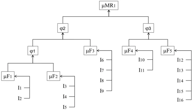
The model relies on THEN rules and arithmetic operators (maximum, weighted sum). The IF-THEN rules are the formalization of expert knowledge. For example, the infiltration phenomenon depends on the watertightness function and drainage function. Thus, if the value of the watertightness function is from 0 to 2, then the infiltration phenomenon takes this value; however, it in fact takes the value of the drainage function. It is a hierarchical model: a global assessment of dam safety deterioration related to different failure modes (denoted
μ
MRk) along with assessments of theperformance of the different technical functions such as sealing, drainage, internal erosion protection and sliding protection (denoted
μ
Fj) are obtained (cf. Figure 1). Intermediate assessments are calledPhenomenon. A model was developed for each deterioration mode. For instance, 9 models were produced for embankment dams. They are related to: Internal Erosion through the Embankment (IEE), Internal Erosion initiated around or near the Spillway (IES), Internal Erosion initiated around or near the Gallery (IEG), Shoulder Sliding (ShS), Overtopping (Ov), Foundation Settlement (FS), Internal Erosion through the Foundation (IEF), Sliding of Embankment and Foundation (SEF), Foundation Plane Sliding (FPS).
Figure 1. Performance assessment using the hierarchical model - Simplistic representation –Ii indicator i –μFj= Performance of Function j –μMRk= Performance related to failure mode MRk – φp= phenomenon
Experts use performance assessment to monitor dam safety and recommend corrective actions if necessary. Corrective actions are of various types and concern both the technical components of the dam and the measurement system (Curt and Talon, 2013; Curt and Gervais, 2014): emergency action (partial or complete emptying of the reservoir), major reconstruction, rehabilitation or safety projects, maintenance actions (scraping of the dowstream slope, drain outlet cleaning, renewal of monitoring equipment and so forth), upgrading dam performance monitoring (increasing measurement frequency, performing laboratory tests and so forth). The objective is twofold: to improve the measurement system (for instance, the scraping of the downstream shoulder allows better visual observations, the renewal of an monitoring device allows obtaining reliable data, etc.) and to guarantee that the performance criteria are satisfied (for instance, the construction of a toe weight allows lengthening water flow and improving performance relative to internal erosion).
2.3.Representation and propagation of imperfections – Expression of outputs
Taking imperfections into account in the assessment procedure is crucial as it leads to better perception than a precise numerical value would do. Indeed, obliging experts to provide precise scores in the case of uncertainty can lead them to give a very bad score in order to conform to the principle of caution. Consequently, corrective actions may be more drastic than they should be.
Three stages are necessary to cope with imperfections: the representation of input imperfections (fuzzification), the propagation in the performance assessment models, and the expression of the outputs (defuzzification).
In the approach developed, the model inputs are indicators. These data are frequently “imperfect”. They contain uncertainty, imprecision, and incompleteness. The fuzzification stage corresponds to the representation of the indicator score and its imperfections as a possibility distribution (cf. Figure 2). A possibility distribution is equivalent to a normalized fuzzy subset (Dubois and Prade, 1988; Zadeh, 1978). The possibility distribution is expressed by the core Cor() and the support Supp(). They
Cor
(
π
I)
=
{
x
∈ X
|
π
I(x )=1
}
(0)Supp
(
π
I)
=
{
x
∈ X
|
π
I( x)> 0
}
(0)For instance, in Figure 2, the core of the trapezoidal distribution is the interval (4; 5) and the support the interval (2; 7).
The distributions are declared by experts on the basis of the indicator grid and photos, in-situ measurement, monitoring curves, etc.
Figure 2. Example of possibility distribution – Most usual frame in the domain of dams
The propagation of possibility distributions via operation f obeys Zadeh’s extension principle (Zadeh, 1978):
π
F(
S
F)
=
¿
(S1,… Sn)|f(S1,… Sn)=SF(
min
(
π
I 1(
S
1)
,… , π
¿(
S
n))
)
(0)with S1,…,Sn being the degradation indicator score and SF, the technical function degradation score. A
model was described for each failure mode (internal erosion through the embankment, shoulder sliding, etc.). At the end of the assessment process, there are as many possibility distributions as there are failure modes.
Figure 3. Example of imperfection propagation in a global dam assessment model – case of internal erosion through the embankment for a homogeneous embankment
The defuzzification phase ends the process. It involves the extraction of a concise and relevant result from the outputs of the performance assessment model. These could be possibility distributions like those presented in Figure 3. As these methods can lead to different results, it is important to make the relevant choice by integrating the future use of the results. Indeed, the final decision is made on the basis of the results obtained.
In our case, the results obtained at the end of imperfection propagation are useful for communication and decision-making concerning dam safety. Experts have to communicate results concerning dam safety to other actors involved in safety, for instance, the dam owner or reservoir operator. They also use these results in view to decision-making: corrective actions must be proposed to restore the dam to standard operating conditions. Consequently, it is essential to properly define the defuzzification method that will be used.
Now that the whole model of dam performance assessment has been described, the next section will focus on the approach taken to develop the last step of this model: defuzzification limited to defining maintenance actions on dams.
3. Approach for the selection of appropriate defuzzification methods
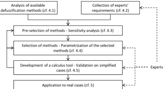
The selection of the most relevant defuzzification methods for application to dams was done with a group of dam experts and an observer responsible for the elicitation and proposal of defuzzification methods. The approach relies on the five phases described in Figure 4; the stages that involve the experts are indicated. They can be iterative:
- Analysis of available defuzzification methods. The first stage aims at identifying the various types of defuzzification approaches (associated with the mean, minimum value, etc.) presented in the literature;
- Collection of the experts’ requirements. A collective session was organized. During this session, the various defuzzification types and methods were presented. The experts broadly expressed their needs and requirements. To refine these proposals, each expert was then invited individually to graphically represent the value that best expresses their requirements for the various possibility distributions proposed;
- Pre-selection of methods on the basis of the two previous stages and, if several methods are candidates, performing a sensitivity analysis for each of them. The objective of the sensitivity analysis is to conserve the most discriminative methods, i.e. the methods that allow the greatest difference between two possibility distributions. The sensitivity analysis considers different experimental possibility distributions that are defuzzified using the pre-selected methods. An experimental design is set up with different values assigned to the parameters of the pre-selected methods if necessary. Finally, an analysis of the dispersion of the results produced by the different methods is performed. Firstly, the effect of the parametrization (when necessary) is determined, which leads to choosing the most discriminative set of parameters for each method. Secondly, the methods can be classified regarding their discriminative ability;
- The proposal of methods in a plenary session, on the basis of the two previous stages. Finally, the appropriate defuzzification methods are selected and the parameters of the methods chosen are determined;
- Development of a calculus tool; validation on simplified cases. The method can then be used on real cases.
Figure 4. Main stages of the approach – Stages involving experts are indicated – Reference of sections dedicated to the explanation of each stage are done
It is noteworthy that the approach can be used for other applications. The following paragraphs describe the various phases of the approach for the assessment of dam performance.
4. Application of the approach to the performance assessment
4.1.Analysis of available defuzzification methods
This stage is totally generic and can be used for other applications. Defuzzification methods can be ranked into four categories: providing a real value, providing a real interval, allowing the ranking of possibility distributions, and methods that assess dispersion.
4.1.1. Methods providing a real value
The purpose of these methods is to extract one relevant value from a fuzzy set. A set of methods was developed and described in (Chandramohan et al., 2006; Leekwijck and Kerre, 1999; Leekwijck and Kerre, 2001; Liu, 2007; Roychowdhury and Pedrycz, 2001). They are listed in Table 3. One can mainly distinguish methods associated with a mean, minimum or maximum value. Methods associated with the mean of the surface or a part of this surface allow representing the global distribution of the fuzzy set; on the contrary, methods associated with a core mean or support mean, or with the minimum or maximum value, only take into account a part of this fuzzy set. Methods associated with the surface mean can be divided into methods using native fuzzy sets and methods in which the fuzzy sets are weighted. The descriptions of each of these methods are given in Appendix A.
Class Subclass Method
Methods associated
to the mean Surface mean Center of Gravity (COG)Center of Area (COA) Midpoint of Area (MOA)
Weighting Function of Center of Gravity (WFCOG)
Maximum Entropy of the Weighting Function of Center of Gravity (MEWFCOG)
Maximum Entropy Weighting Function of the Basic Defuzzification Distribution (MEWFBADD)
Fuzzy Mean (FM)
Weighted Fuzzy Mean (WFM) Quality Method (QM)
Extended Quality Method (EQM) A part of the
surface mean Indexed Center of Gravity (ICOG) Support mean Mean of Support (MOS or MeOS)
Core mean Mean of Maxima or Middle of Maximan (MOM or MeOM) Continuity Focused Choice Of Maxima (CFCOM)
Center of Mean (COM) Surface or core or
support mean (depending of parameter value)
Extended Center of Area (ECOA)
Basic Defuzzification Distribution (BADD) Generalized Level Set Defuzzification (GLSD) Random Generation (RAGE)
Semi-linear Defuzzification (SLIDE) Methods associated
to the minimum First of Maxima (FOM)First of Support (FOS) Methods associated
to the maximum Last of Maxima (LOM)Last of Support (LOS)
Other methods Constraint Decision Defuzzification (CDD) Root Mean Square 1 (RMS1)
Root Mean Square 2 (RMS2) Fuzzy Cluster-Means (FCM)
Random Choice of Maxima (RCOM)
4.1.2. Methods providing a real interval
The aim of defuzzification methods that provide a real interval is to achieve the best representation of the dispersion of the fuzzy set. Five defuzzification methods are available (detailed in Appendix B): the formulation of Dubois and Prade (1987), the formulation of Carlson and Fuller (2002), that of Bodjanova (2005), that of Grzegorzewski (2002), and that of Chanas (2001).
These methods are interesting as they allow representing all the information of a fuzzy set; nevertheless, the resulting interval is very wide. Indeed, it generally fills the width of several units while the decision-making basis for our case study is the unit or possibly the score (including two or three units).
4.1.3. Methods allowing the ranking or comparison of possibility distributions
In the context of our case study the aim of possibility distribution ranking methods is to both order the set of fuzzy sets and assign a membership class to them. Three kinds of fuzzy set ranking methods are available.
The first type of ranking method proceeds with defuzzification, leading to a real value and then ranking the fuzzy sets using the real values obtained. Methods used to obtain a real value have been presented previously. Then, the real values are ranked in increasing or decreasing order. The results are necessarily strongly linked to the choice of the initial defuzzification method. This first type of method allows ordering a set of fuzzy sets.
The second type of method compares fuzzy sets to one (or several) reference fuzzy sets. Major references of these methods are (Chen and Lu, 1999; Fortemps and Roubens, 1996; Wang and Kerre, 2001a; Wang and Kerre, 2001b). We consider that only two methods are relevant for our case study: standard compatibility degree (Curt, 2013) and distance minimization (Fortemps and Roubens, 1996). The first method allows obtaining a percentage of membership to a class and the second provides a partial order between two probability distributions. The other methods are quite similar to either one or the other of these two methods, though they do not possess parameters that allow comparing their sensitivity. Appendix C gives more details on each of them. These kinds of method provide the membership of a fuzzy set to a class but do not directly order the fuzzy sets.
The third type of method compares fuzzy sets two by two. Major references of these methods are (Abbasbandy et al. 2006; Asady and Zendehnam, 2007; Dubois and Prade, 1983; Wang and Kerre, 2001a; Wang and Kerre, 2001b). Only one method seems to be relevant for our case study, namely distance minimization by sign (Abbasbandy et al. 2006). Indeed, other methods have been developed for a particular application but are very difficult to apply to our problematic. This type does not take into account the whole membership function. Equivalence between several fuzzy sets can appear but these methods do not provide a total order.
4.1.4. Dispersion assessment methods
The aim of fuzzy set dispersion assessment methods, in the context of our application, is to distinguish several fuzzy sets having the same real value of defuzzification but a distinct frame and therefore distinct uncertainty. Three kinds of methods can be distinguished: relative entropy, based on Shannon’ entropy (Shannon, 1948), relative surface, and mean distance to the gravity center (Appendix D). In the context of our study, entropy is used to assess the certainty that one can assign to a datum (a possibility distribution). The certainty of a datum is considered as proportional to the dispersion of its membership in the discernment frame; that is to say that a datum centered on a value will present more certainty than an interval that includes this value (that introduces more uncertainty into the assessment).
The aim of the methods based on relative surface is to assess the surface of a fuzzy set in comparison with the surface of the whole scale of assessment.
4.2.Collection of expert requirements and pre-selection of methods
Here, the objective is to propose methods that meet experts’ requirements. Experts need several kinds of information that allow interpreting the performance of a dam, regarding a failure mode, expressed as a fuzzy frame:
- For decision-making: there are as many possibility distributions as there are models (one model per failure mode). To conduct their reasoning, the experts want to have all the information, that is to say the graphic representation of the resulting fuzzy set, and they want to order the fuzzy sets in relation to each other, as the distributions are expressed on commensurable scales. Methods used for comparing fuzzy sets to reference fuzzy sets (standard compatibility degree and distance minimization) do not allow ordering fuzzy sets in relation to each other. However, methods that proceed from a combination of two steps, i.e. defuzzication to obtain a real value and ordering are particularly interesting from the quantitative point of view and are thus selected.
- Regarding the transmission of information to dam managers, the requests are the following: representation of the whole distribution and an expression of its dispersion. Methods providing a real value or a real interval are pertinent for representing all the information included in the distribution. Finally, all the methods used to calculate dispersion seem convenient for our application. To facilitate information transmission, it is also proposed that a qualitative expression be associated with the quantitative values extracted by the defuzzification methods. This last step completes the defuzzification process: for instance, the modification of the defuzzified value on a qualitative scale ranging from “no dispersion” to “very high dispersion”. This process is carried out for each model output.
Thus the various methods of the four types of defuzzification process can be candidates. An initial selection can be performed for methods providing real value. Since a request of experts is to consider the whole distribution, attention is given to the methods associated with the whole part of the mean, while the other approaches (associated with the minimum and maximum, and the other methods presented in Table 3) are not considered. Some methods associated with the mean are similar to each other. The following presents the equivalences: the COG, COA and MOA methods are equivalent and take into account the whole native fuzzy set. The WFCOG method allows weighting the x values of a fuzzy set. The MEWFCOG method calculates the maximum entropy of function
f ( x )
that shows the weighting of the x values of the fuzzy set, with∫
a b
f ( x) dx=1
where a and b are the limits of the given fuzzy set. In addition to the WFCOG method, functionf ( x )
, with coefficient λ, allows showing the decision-maker’s point of view: 0 for a pessimistic point of view, 0.5 for a neutral point of view and > 0.5 for an optimistic point of view (which lead to the highest weights). The MEWBADD method is similar to the NEWFCOG method.FM method corresponds to an optimization of the COG method. The WFM method allows taking into account weights associated with each value x of the fuzzy set. The QM method is close to the WFM method where the weights are equal to the opposite of the support width. The EQM method is an expansion of QM where
ξ
∈
¿
allow influencing the importance assigned to support. Forξ=0
, the EQM method is similar to the FM method (support width is not taken into account), for ξ=1, the EQM method is similar to the QM method and forξ >1
, the support width takes a very high value. Two main methods deal with a part of the surface mean: the ICOG method corresponds to the COG method where only the values higher than a given -cut are taken into account.Some methods lead to using the mean (complete or part) and the core of the support as a function of the value of a parameter. The ECOA method is an extension of the COA method where the factor
γ∈¿ helps to take into account the confidence assigned to the fuzzy set. For a value γ=0 the support mean will be taken; for
γ=1
the mean of the whole fuzzy set will be taken and forγ →∞
the core mean will be taken. The SLIDE method allows taking into account values under a given -cut andhigher or lower values above this -cut by using a parameter
β
∈
[
0 ;1
]
. The SLIDE method is similar to:- COG method for
α=0∧
∀ β ∈
[
0 ;1
]
and forβ=0∧
∀ α ∈
[
0 ;h ( A )
]
where A is a fuzzy set; - ICOG method forβ=1∧∀ α ∈
[
0 ;h ( A )
]
;- MeOM method for
β=1∧α=h ( A )
.The BADD and GLSD methods are similar to the ECOA method. The RAGE method is close to the BADD and SLIDE methods.
Methods that allow weighting the weight granted to the different values of the membership function allow stressing the importance granted to the more probable values (-cuts nearest the core, i.e. nearest to
μ ( x )=1
).To go further in the selection, a sensitivity analysis is performed for categories for which different methods are candidates, i.e. methods providing a real value, methods providing an interval, methods allowing ranking or comparing possibility distributions and dispersion assessment.
4.3.Sensitivity analysis of defuzzification methods
The sensitivity analysis relies on different experimental possibility distributions and an experimental design set up with different values assigned to the parameters of the pre-selected methods if necessary: several cases are defined. Finally, an analysis of the dispersion of the results produced by the different methods is performed.
4.3.1. Experimental possibility distributions
The sensitivity analysis is performed using six characteristic possibility distributions (PD) presented in Figure 5. They are termed characteristic as they represent the frames (rectangular, triangular or trapezoidal) encountered in our dam application; as possibility distributions, their height is standardized to 1. Moreover, they allow representing the two main variable parameters: the width of the support and the width of the core. Possibility distributions 1 to 3 allow representing the variation of core width with the same support width. Possibility distributions 1 and 4, 2 and 6, 3 and 5, respectively, have the same core widths and distinct support widths.
Possibility distribution 1 Possibility distribution 2
Possibility distribution 5 Possibility distribution 6
Figure 5. Possibility distributions used for the sensitivity analysis – These are the most usual frames used in dam assessment – The possibility distributions vary from their core widths and support widths
4.3.2. Experimental design: methods providing a real value
Methods providing a real value integrate intrinsic parameters that are distinct from the variation of the support and core widths. This sensitivity analysis also consists in studying the variation of these parameters.
These intrinsic parameters are:
f ( x )
(function of weight associated with each value of membership), -cuts,w
i (weight associated with each -cut), (given -cut), , , , (parameters that allowinfluencing the importance assigned to certain membership values of a fuzzy set). The parameters to be defined for each defuzzification method, in addition to the membership function, are listed in Table 4. COG, COA, MOM, MOS only require the membership function. The MOA, RAGE and COM methods were not studied, as they are similar to the COG, BADD and MOM methods, respectively. Also, the CDD and FCM methods were not studied as they do not correspond to the type of method sought (constraints are not considered and the number of data handled is relatively low). For the root mean square (1 and 2) methods, RMS1 provides the membership value of RMS2. Consequently, only RMS2 is comparable to the other method results, and so only the sensitivity of RMS2 is studied. Along the same lines, the RCOM method provides the probability that a chosen value x0 is included in
the core of the fuzzy set. Consequently, this method is of no interest to us. Parameters Methods
f ( x )
WFCOG, MEWFCOG, MEWFBADD-cuts GLSD, FM, WFM, QM, EQM, CFCOM
w
i WFM ICOG, SLIDE
SLIDE
EQM
MEWFCOG
ECOA, BADD, MEWFBADD, GLSD
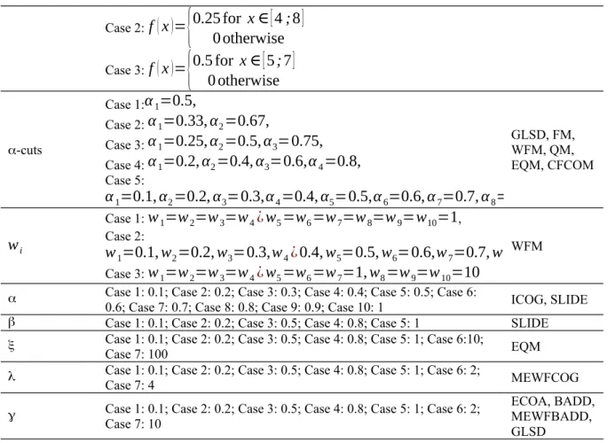
Table 4. The parameters needed to define the defuzzification methods and corresponding methods The experimental design applied to the six possibility distributions of Figure 5 is summarized in Table 5. This experimental design was chosen to exploit all the possibilities of the different defuzzification methods.
Parameters Values Methods
f ( x )
Case 1:f ( x )=0.1 for x
∈
[
0;10
]
WFCOG,Case 2:
f ( x )=
{
0.25 for x
∈
[
4 ;8
]
0 otherwise
Case 3:f ( x )=
{
0.5 for x
∈
[
5 ;7
]
0 otherwise
-cuts Case 1:α
1=0.5,
Case 2:α
1=0.33, α
2=0.67,
Case 3:α
1=0.25, α
2=0.5, α
3=
0.75,
Case 4:α
1=0.2, α
2=0.4, α
3=0.6,α
4=0.8,
Case 5: α1=0.1, α2=0.2, α3=0.3,α4=0.4, α5=0.5,α6=0.6, α7=0.7, α8=0.8, α9=0.9, α10=1 GLSD, FM, WFM, QM, EQM, CFCOMw
i Case 1:w
1=
w
2=
w
3=
w
4¿
w
5=
w
6=
w
7=
w
8=
w
9=
w
10=1
, Case 2:w
1=0.1, w
2=0.2, w
3=
0.3,w
4¿
0.4, w
5=0.5, w
6=0.6,w
7=0.7, w
8=0.8, w
9=0.9, w
10=1,
Case 3: w1=w2=w3=w4¿w5=w6=w7=1, w8=w9=w10=10 WFM Case 1: 0.1; Case 2: 0.2; Case 3: 0.3; Case 4: 0.4; Case 5: 0.5; Case 6:
0.6; Case 7: 0.7; Case 8: 0.8; Case 9: 0.9; Case 10: 1 ICOG, SLIDE Case 1: 0.1; Case 2: 0.2; Case 3: 0.5; Case 4: 0.8; Case 5: 1 SLIDE Case 1: 0.1; Case 2: 0.2; Case 3: 0.5; Case 4: 0.8; Case 5: 1; Case 6:10;
Case 7: 100 EQM
Case 1: 0.1; Case 2: 0.2; Case 3: 0.5; Case 4: 0.8; Case 5: 1; Case 6: 2;
Case 7: 4 MEWFCOG
Case 1: 0.1; Case 2: 0.2; Case 3: 0.5; Case 4: 0.8; Case 5: 1; Case 6: 2; Case 7: 10
ECOA, BADD, MEWFBADD, GLSD
Table 5. Cases studied to analyze the variation of the defuzzification method parameters – All the possibilities of deffuzification methods to be tested
4.3.3. Results concerning methods providing a real value
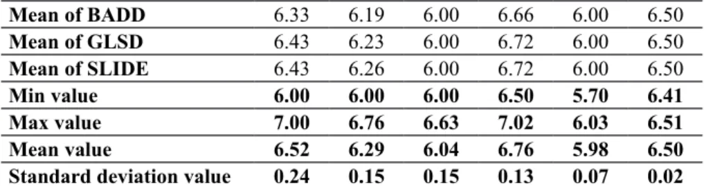
The results obtained by the methods providing a real value referenced in Appendix A are given in Table 6. Table 6 provides the mean value of the different cases tested for the methods of the Table 5. For each possibility distribution, the minimum value, the maximum value, the mean value and the standard deviation value of all the methods analyzed are also given.
Possibility distribution PD 1 PD 2 PD 3 PD 4 PD 5 PD 6 COG 6.33 6.20 6.00 6.67 6.00 6.50 COA 6.45 6.25 6.00 6.74 6.00 6.50 MOS 6.00 6.00 6.00 6.50 6.00 6.50 MOM 7.00 6.50 6.00 7.00 6.00 6.50 RMS2 6.39 6.26 6.07 6.70 6.03 6.51 Mean of WFCOG 6.39 6.23 6.00 6.63 6.00 6.50 Mean of MEWFCOG 6.96 6.76 6.63 7.02 5.70 6.41 Mean of MEWBADD 6.39 6.22 6.00 6.62 6.00 6.50 Mean of FM 6.59 6.29 6.00 6.79 6.00 6.50 Mean of WFM 6.63 6.31 6.00 6.81 6.00 6.50 Mean of QM 6.64 6.31 6.00 6.82 6.00 6.50 Mean of EQM 6.64 6.32 6.00 6.82 6.00 6.50 Mean of ICOG 6.62 6.33 6.00 6.81 6.00 6.50 Mean of CFCOM 6.74 6.37 6.00 6.87 6.00 6.50 Mean of ECOA 6.41 6.23 6.00 6.71 6.00 6.50
Mean of BADD 6.33 6.19 6.00 6.66 6.00 6.50 Mean of GLSD 6.43 6.23 6.00 6.72 6.00 6.50 Mean of SLIDE 6.43 6.26 6.00 6.72 6.00 6.50 Min value 6.00 6.00 6.00 6.50 5.70 6.41 Max value 7.00 6.76 6.63 7.02 6.03 6.51 Mean value 6.52 6.29 6.04 6.76 5.98 6.50
Standard deviation value 0.24 0.15 0.15 0.13 0.07 0.02
Table 6. Results of methods providing a real value: mean for each method, min, max, mean and standard deviation of all the methods – The PDi correspond to the possibility distributions given
in Figure 5
The different methods provide a homogeneous result for possibility distributions 5 and 6 except for RMS2 and NEWFCOG that have a difference of 0.03 and 0.3, respectively, for possibility distribution 5 and 0.01 and 0.09 for possibility distribution 6. Regarding the possibility distributions from 1 to 4, the method that provides the most optimistic value (the nearest to 0 on our scale from 0 to 10) is MOS. On the contrary, the method that provides the most pessimistic value is MOM for the PD1 and MEWFCOG for PD2 to PD4. PD1, 2 and 3 have the same support but different cores, the core of PD1 is centered on 7, the core of PD2 is centered on 6-7 and the core of PD3 is centered on 5-7. The certainty of going from PD1 to PD3 extends to the lowest values. This aspect is well represented by the different methods as the mean value of defuzzification for PD1 (6.52) is higher than for PD2 (6.29) which is higher than that of PD3 (6.04). For PD1 and PD4, the core is the same (7) and the support is larger for PD4 (4-8) than for PD4 (5-8) while the uncertainty for PD1 extends to the optimistic values in comparison to PD4. This aspect is well represented by the different methods as the mean value of defuzzification for PD4 (6.76) is higher than for PD1 (6.52). By comparing the results for PD3 and PD5, the different methods allow taking into account the “symmetric” uncertainty associated with PD3 by assigning a defuzzification value on average higher (6.04) than for PD5 (5.98).
By comparing the results for PD2 and PD6, the different methods tend to extend the defuzzification value on average to the higher uncertainties: 6.29 for PD2 which has a support of 4-8 in comparison to 6.5 for PD3 which has a support of 5-6. Both PDs have the same core (5-6). In every case, the standard deviation values are very low and therefore all the methods tested provide the precision expected by the experts, i.e. close to the unit.
Table 7 provides the mean defuzzification values, their extents and their standard deviations (SD) for the six possibility distributions when the parameters of Table 5 vary.
PD1 PD2 PD3 PD4 PD5 PD6 WFCOG Mean 6.39 6.23 6.00 6.63 6.00 6.50 Extent 0.17 0.09 0.00 0.11 0.00 0.00 SD 0.10 0.05 0.00 0.06 0.00 0.00 MEWFCOG Mean 6.96 6.76 6.63 7.02 5.70 6.41 Extent 0.81 0.84 1.12 0.51 0.72 0.26 SD 0.34 0.32 0.46 0.20 0.26 0.09 MEWFBADD Mean 6.39 6.22 6.00 6.62 6.00 6.50 Extent 0.80 0.42 0.00 0.61 0.00 0.00 SD 0.24 0.13 0.00 0.17 0.00 0.00 FM Mean 6.59 6.29 6.00 6.79 6.00 6.50 Extent 0.20 0.10 0.00 0.10 0.00 0.00 SD 0.07 0.04 0.00 0.04 0.00 0.00
WFM Mean 6.63 6.31 6.00 6.81 6.00 6.50 Extent 0.37 0.18 0.00 0.18 0.00 0.00 SD 0.11 0.05 0.00 0.05 0.00 0.00 QM Mean 6.64 6.31 6.00 6.82 6.00 6.50 Extent 0.27 0.14 0.00 0.13 0.00 0.00 SD 0.10 0.05 0.00 0.05 0.00 0.00 EQM Mean 6.64 6.32 6.00 6.82 6.00 6.50 Extent 0.40 0.25 0.00 0.20 0.00 0.00 SD 0.11 0.06 0.00 0.05 0.00 0.00 ICOG Mean 6.62 6.33 6.00 6.81 6.00 6.50 Extent 0.66 0.30 0.00 0.33 0.00 0.00 SD 0.23 0.10 0.00 0.11 0.00 0.00 CFCOM Mean 6.74 6.37 6.00 6.87 6.00 6.50 Extent 0.50 0.25 0.00 0.25 0.00 0.00 SD 0.18 0.09 0.00 0.09 0.00 0.00 ECOA Mean 6.41 6.23 6.00 6.71 6.00 6.50 Extent 0.81 0.41 0.00 0.41 0.00 0.00 SD 0.28 0.14 0.00 0.14 0.00 0.00 BADD Mean 6.33 6.19 6.00 6.66 6.00 6.50 Extent 0.78 0.42 0.00 0.40 0.00 0.00 SD 0.27 0.14 0.00 0.14 0.00 0.00 GLSD Mean 6.43 6.23 6.00 6.72 6.00 6.50 Extent 0.77 0.43 0.00 0.39 0.00 0.00 SD 0.18 0.09 0.00 0.09 0.00 0.00 SLIDE Mean 6.43 6.26 6.00 6.72 6.00 6.50 Extent 0.57 0.30 0.00 0.28 0.00 0.00 SD 0.13 0.07 0.00 0.06 0.00 0.00
Table 7. Results of methods providing a real value: mean, extent and standard deviation for the variation of parameters of Table 5 – The PDi correspond to the possibility distributions given in
Figure 5
For almost all the methods (except MEWFCOG) the variation of parameters has no influence on the defuzzification value when the possibility distributions are symmetrical: possibility distributions 3, 4 and 6. For WFCOG and MEWFBADD and PD1, 2 and 4, the defuzzification value is attracted by the larger values of function
f ( x )
. For GLSD, FM, WFM, QM, EQM and CFCOM and PD1, PD2 and PD4, the defuzzification value increases as the -cuts number increases. For WFM, the variation ofw
i has little influence on the variation of the defuzzification value. For ICOG and PD1, 2 and 4, the defuzzification value increases as increases. For SLIDE and PD1, 2 and 4, the defuzzification value varies little with the variation of ; on the contrary, it increases as increases. For EQM, the variation of ξ has little influence on the variation of the defuzzification value. For MEWFCOG, the defuzzification value increases from the COG value to the upper bound of the support when the value of λ increases. For MEWFBADD, ECOA, BADD and GLSD and PD1, 2 and 4, the defuzzification values increase as the value ofγ
increases.4.3.4. Results of methods providing a real interval
The results obtained by the methods providing a real interval referenced in Appendix B are given in Table 8. The resulting interval for each method and each possibility distribution of Figure 5 are provided. Moreover, for each possibility distribution, the mean values of the lower and upper bounds of the intervals of all the methods and their standard deviations are calculated.
Possibility distribution PD 1 PD 2 PD 3 PD 4 PD 5 PD 6
Dubois and Prade (5.5 ; 7.5) (5 ; 7.5) (4.5 ; 7.5) (6 ; 7.5) (5 ; 7) (6 ; 7)
Carlson and Fuller (6 ; 7.33) (5.33 ; 7.33) (4.67 ; 7.33) (6.33 ; 7.33) (5 ; 7) (6 ; 7)
Bodjnova (6.12 ; 7.29) (5.41 ; 7.29) (4.71 ; 7.29) (6.41 ; 7.29) (5 ; 7) (6 ; 7)
Grzegorzewski (5.5 ; 7.5) (5 ; 7.5) (4.5 ; 7.5) (6 ; 7.5) (5 ; 7) (6 ; 7)
Chanas (5.5 ; 7.5) (5 ; 7.5) (4.5 ; 7.5) (6 ; 7.5) (5 ; 7) (6 ; 7)
Mean value of lower bound 5.72 5.15 4.58 6.15 5 6
Mean value of upper bound 7.42 7.42 7.42 7.42 7 7
Standard deviation of lower
bound 0.31 0.20 0.11 0.20 0 0
Standard deviation of upper
bound 0.11 0.11 0.11 0.10 0 0
Table 8. Results of methods providing a real interval: interval of values for each method, mean and standard deviation for the lower and upper bounds of all the methods – The PDi correspond
to the possibility distributions given in Figure 5
The methods providing an interval are interesting in order to take into account the dispersion of fuzzy sets. For our application the scale of discrimination between two values is in the range of the unit. The standard deviation of the mean values of the lower and upper bounds of the intervals obtained by the different methods are at most equal to 0.31. From our viewpoint, these different methods are therefore equivalent.
4.3.5. Results of methods used to rank or compare possibility distributions
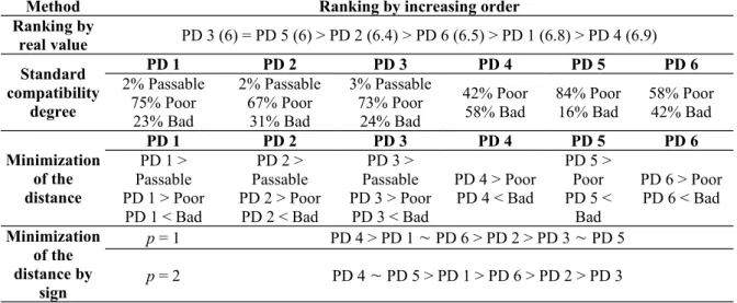
The results obtained with methods used to rank or compare possibility distributions detailed in Appendix C for the six possibility distributions of Figure 5 are given in Table 9. Ranking by increasing order of values is performed: the value nearest 0 corresponds to a dam in “very good state”, which is preferred to a dam in “unacceptable state” (score of 10).
Method Ranking by increasing order
Ranking by real value PD 3 (6) = PD 5 (6) > PD 2 (6.4) > PD 6 (6.5) > PD 1 (6.8) > PD 4 (6.9) Standard compatibility degree PD 1 PD 2 PD 3 PD 4 PD 5 PD 6 2% Passable 75% Poor 23% Bad 2% Passable 67% Poor 31% Bad 3% Passable 73% Poor 24% Bad 42% Poor
58% Bad 84% Poor16% Bad 58% Poor42% Bad
Minimization of the distance PD 1 PD 2 PD 3 PD 4 PD 5 PD 6 PD 1 > Passable PD 1 > Poor PD 1 < Bad PD 2 > Passable PD 2 > Poor PD 2 < Bad PD 3 > Passable PD 3 > Poor PD 3 < Bad PD 4 > Poor PD 4 < Bad PD 5 > Poor PD 5 < Bad PD 6 > Poor PD 6 < Bad Minimization of the distance by sign p = 1 PD 4 > PD 1 PD 6 > PD 2 > PD 3 PD 5 p = 2 PD 4 PD 5 > PD 1 > PD 6 > PD 2 > PD 3
Table 9. Results of methods of ranking or comparing possibility distributions – The PDi correspond to the possibility distributions given in Figure 5
For the calculation of the ranking method by real values, the method selected is the mean of the -cut at 0.8. The explanation for choosing this method is given in 4.4. In Table 9, the number between brackets near the case number corresponds to the defuzzified value (mean of the -cut at 0.8).
The selected reference fuzzy sets are presented in Figure 6. These classes are those commonly used by experts for characterizing the state of dams.
Methods of comparing fuzzy sets to reference fuzzy sets (standard compatibility degree and distance minimization) do not allow ordering fuzzy sets in relation to each other. The standard compatibility degree method is used to quantify the membership of a fuzzy set in the reference classes (defined with the reference fuzzy sets), contrary to the distance minimization method. Except for possibility distribution 5, the ranking obtained with the distance minimization method by sign is similar even if p is equal to 1 or to 2.
Although ranking by real value is inverted when applying the distance minimization method by sign, the ranking obtained is similar. This inversion stems from the fact that the scale of our case study (and thus the method of ranking by real value) is better for a score of 0 than for a score of 10.
4.3.6. Results of dispersion assessment methods
The results obtained with dispersion assessment methods described in Appendix D for the six possibility distributions of Figure 5 are given in Table 10.
Possibility Distribution PD 1 PD 2 PD 3 PD 4 PD 5 PD 6
Relative entropy 0.52 0.53 0.55 0.39 0.30 0.00
Relative surface 2.00 2.50 3.00 1.50 2.00 1.00
Mean distance to the center of gravity 1.00 1.25 1.50 0.75 1.00 0.50
Table 10. Results of dispersion methods – The PDi correspond to the possibility distributions given in Figure 5
In our context, when the experts provide fuzzy sets, possibility distributions 1 to 4 correspond to a dispersion that is rather considerable when possibility distributions 5 and 6 represent knowledge of relative certainty for the values given to the indicators. Only the relative entropy method allows making this distinction. Indeed, regarding the methods of relative surface and mean distance to the center of gravity, the values obtained for possibility distributions 1 and 5 are the same whereas the signification associated with these two possibility distributions is different for the experts.
Once the pre-selected defuzzification methods have been subjected to a sensitivity analysis, it is then possible to select the relevant methods for our application of dam performance assessment.
4.4.Selection of methods and parameterization
The selected defuzzification methods are presented in Table 11.
The value of 0.8 for the -cut was chosen by the experts for decision-making and communication purposes. This was done considering the correspondence between the percentiles (probability approach) and membership values (possibility approach) as defined in (Baudrit et al., 2003; Vick, 1997) and presented in Table 12. Indeed, the experts chose a defuzzification value that corresponds to a value between “averagely probable” and “probable”. The mean of the -cut at 0.8 was chosen to correspond to the experts’ requests: a value to the right of the COG and as far from it as the dispersion is high.
Type of result Type of information Method selected
Decision making Qualitative Graphic representation
Quantitative Defuzzification with real value by the mean -cut at 0.8 and ranking by increasing order (from the lowest value, nearest to 0, to the highest value, nearest to 10) of the real
values.
Communication
Quantitative – score Defuzzification by the upper limit of the -cut at 0.8 Quantitative – dispersion Relative entropy
Qualitative – dispersion
Interpretation of the relative entropy (no dispersion, low dispersion, high dispersion, very high dispersion) regarding the entropy value.
Qualitative – membership Calculus of the percentage of membershipto the assessment classes of indicators by the standard compatibility degree.
Table 11. Defuzzification methods Selected by expert group for the assessment of dam performance – There are sets of qualitative and quantitative methods for both objectives: decision-making and
communication to dam managers
Linguistic meaning Percentiles Membership values
Practically impossible 1% 0.02 Very improbable 10% 0.20 Improbable 15% 0.30 Rather improbable 25% 0.50 Averagely probable 50% 1.00 Probable 75% 0.50 Rather probable 80% 0.40 Very probable 90% 0.20 Practically certain 99% 0.02
Table 12. Correspondence between percentiles (probability approach) and membership values (possibility approach) based on the works of (Baudrit et al., 2003; Vick, 1997)
For the purposes of communication, the expected values must be to the right of the center of gravity in order to take into account the safety aspect; the distance to the center of gravity must be as large as the dispersion is high. The upper limit of the -cut at 0.8 was chosen in order to ensure a correspondence between this approach and the approach selected for the expert reasoning, but with a higher level of safety (indeed, the upper limit of the -cut must be higher than or equal to the mean of the -cut). Relative entropy was chosen to quantify the dispersion of the fuzzy set as it evolves proportionally as its dispersion increases, contrary to the other methods. In particular, in the context of our case study, there is a big difference between the support and the core, characterizing high uncertainty for the expert during their assessment.
We propose to facilitate the transmission of information using a qualitative expression associated with the quantitative values extracted by defuzzification methods.
The approach used to translate the quantitative score into a qualitative one is performed by projecting the precise score obtained onto the scale presented in Figure 6.
Figure 6. Fuzzy sets describing the qualitative scale associated with the quantitative score. This scale is used for the calculus of the percentage of membership of the classes of indicators used in the assessment
by the standard compatibility degree
A qualitative interpretation of the dispersion value for communication is also provided through four qualitative classes: no dispersion, poor dispersion, high dispersion, very high dispersion.
The quantitative limits of these qualitative classes are set using the fuzzy sets “of reference” presented in Table 13. The associated values of relative entropy are also indicated in Table 13.
Class Fuzzy set of reference Value of relative
entropy No dispersion 0 Poor dispersion 0 – 0.30 High dispersion 0.30 – 0.44 Very high dispersion Beyond > 0.44
Table 13. Class limits of the qualitative interpretation of dispersion – The fuzzy sets of reference were defined by experts. A class (like“High dispersion”) is associated with these fuzzy sets of reference and then
the correspondence is made from the qualitative interpretation and the value of relative entropy 4.5.Development of a calculus tool and validation on simplified cases
A tool was developed with Visual Basic that allows calculating the results of the methods selected by the experts (cf. 4.4) by implementing all the indicators relevant to a dam in the framework of fuzzy sets.
The tool was tested on a set of academic cases (dams with few indicators) in order to present its outputs to the experts and to validate its pertinence regarding with their expectations.
5. Application to a real case study
This section describes how the defuzzification stage takes place in the whole model of dam performance assessment. The case study is presented, then the outputs of the model are indicated – those useful for the defuzzification phase – and finally the results of the deffuzication phase are given. 5.1.Description of the case study
The dam considered (called Example Dam) is a homogeneous dam, 15.5 m high, impounding a 3.6 hm3 lake, with an upstream embankment built of dirty, silty sand and a downstream embankment built of clean, silty sand. The upstream shoulder is covered with rip-rap protection placed on a geotextile.
The downstream embankment is protected by grass. The dam has a vertical drain and a drainage blanket at the interface of the foundation with the downstream embankment. It is equipped with a reinforced concrete, frontal spillway. The foundation has a granite arena structure. It is sealed by grouting.
The monitoring system is composed of 18 survey points built on the work and 4 benchmarks on the left side to control altimetry displacements, 7 pressure cells, 13 piezometers located on the left and right sides, completed later with 3 piezometers placed on the downstream embankment (after the occurrence of a leak in this zone), and drain monitoring (6 measurements).
4 years after the reservoir was filled, a wet area without apparent leakage was observed at the downstream toe. During the following years, the damp patch grew larger, and localized slides and seepages could be observed on the upstream shoulder. The assessment presented below was performed on the data collected 20 years after the reservoir was filled, on the occasion of a full review of the dam.
5.2.Assessment indicators and calculation of performances related to failure mode
The indicators are assessed on the basis of the report written by an expert at the end of the full review. Once the indicators have been assessed, the performances related to each failure mode are calculated using models such as that presented in Figure 1. The detailed results obtained to assess internal erosion through the embankment are represented as a graph in Figure 3. Three indicators are assessed as triangular distributions (flow decrease, seepage of clean water, piezometry); one as an imprecise interval (differential settlement) and the seven others as precise scores. Possibility distributions representing the indicator scores are propagated in the model: two functions (Drainage and Erosion Defense) are computed as possibility distributions and the other (Sealing) as a precise score. Finally, the assessment of internal erosion through the embankment is an imprecise interval. Figure 3 shows that the Drainage and the Erosion Defense Functions dysfunction.
Failure mode Model output
Internal erosion through the embankment (IEE) 1 0.75 0.5 0.25 2 4 6 8 10 0 Shoulder sliding (ShS) 1 0.75 0.5 0.25 2 4 6 8 10 0
Internal erosion initiated around or near the spillway (IES) 1 0.75 0.5 0.25
2 4 6 8 10 0
Internal erosion initiated around or near the gallery (IEG) 1 0.75 0.5 0.25
2 4 6 8 10 0
Internal erosion through the foundation (IEF) Sliding of embankment and foundation (SEF) Overtopping (Ov)
Foundation Settlement (FS) Foundation Plane Sliding (FPS)
Table 14. Assessment of performances related to failure mode for the Example Dam – qualitative representation for decision-making
The same process is applied for the whole set of failure modes. The results of these calculations are listed in Table 14. Three out of nine are calculated as possibility distributions, IEE, IES, ShS while the others are precise scores.
5.3.Defuzzification
The defuzzified data are presented in Table 15.
Four model outputs are higher than 2, corresponding to the class “Good” on the assessment scale: IEE, IES, ShS and IEG. These results express abnormal behavior; they are explained in particular by the detection of seepages (on the downstream embankment, near the spillway and in the gallery) and the presence of local surface creep on the downstream embankment. The other functions perform properly. Table 14 and Table 15 show that the situation is critical concerning IEE and serious for ShS. Dispersion is low for all the results. This is a particularly interesting result of the study: it means that the conclusions concerning the situation relative to IEE and ShS are fair.
Aims Type of results Results
Decision-making Quantitative representation
(QR) Ranking from the most deteriorated function to the less one Symbol ≈ means the functions present same performance QR IEE > QR ShS > QR IES > QR IEG > QR IEF ≈ QR SEF ≈ QR Ov ≈ QR FS ≈ QR FPS
Communication Quantitative score (QtS) QtS IEE = 9; QtS ShS = 5.8; QtS IES = 4; QtS IEG = 3
QtS IEF = QtS SEF = QtS Ov = QtS FS = QtS FPS = 2
Quantitative dispersion
(QtD) QtD QtD ShSIEE = 0.05 = QtD IES = 0.1
QtD IEG = QtD IEF = QtD SEF = QtD Ov = QtD FS = QtD FPS = 0
Qualitative dispersion
(QlD) QlDQlD IEG =IEE = QlD QlD IEF = ShS = QlD QlD SEF = IES = “Low dispersion” QlD Ov = QlD FS = QlD FPS = “No
dispersion” Qualitative membership
(QlM)
QlM IEE = 100% “Bad”
QlM ShS = 100% “Poor”
QlM IES = QlS IEG = 100% “Passable”
QlM IEF = QlS SEF = QlS Ov = QlS FS = QlS FPS = 100 % “Good” Table 15. Results of the defuzzification process for the example dam of Table 14
At the end of the review, emergency corrective actions were proposed by experts: they concerned lowering the reservoir. Works have to be performed on the drainage system that was identified as the origin of the IEE and ShS problems. The measurement system was not concerned by corrective actions.
6. Conclusion
This article proposed an approach for the selection of a defuzzification method to provide usable output forms. The first section described the dam performance assessment model. The outputs of this model are fuzzy sets that have to be defuzzified so that the dam experts can decide the maintenance actions to be carried out and communicate their decision to the dam managers. The second section is dedicated to the approach taken to select relevant defuzzification methods: the analysis of all defuzzification methods, the collection of expert requirements, the pre-selection of methods, sensitivity analysis of pre-selected methods, the development of a tool to facilitate the analysis. Then, the sensitivity analysis and the justification for selecting the methods were described. Finally, a real case study was presented to illustrate the use of the defuzzification methods selected in the whole dam performance assessment model. Although numerous defuzzification methods have been described in the literature, they have usually been applied using standard methods, centroids or means of maxima.
Few works deal with the problem of choosing defuzzification methods and our approach to their selection is new: the methodology strongly involved experts. Experts were involved in the definition of the objectives of defuzzification: two were defined, i.e. communication and decision-making to propose corrective actions. They were also asked to choose from the defuzzication methods collected in the literature. Moreover, our methodology relied on a sensitivity analysis to improve the choice between different methods of the same type. The approach developed here for the sensitivity analysis was performed on quite a large number of preselected methods, but it could be applied to other defuzzication methods. The research was applied to the assessment of dam performance based on dam failure modes but it can be applied to other systems, notably through the possible use of a sensitivity analysis of the different defuzzication methods presented here and of methodological reasoning.
7. References
Abbasbandy, S., Asady, B. (2006). Ranking of fuzzy numbers by sign distance. Information Sciences 176, 2405-2416.
Amaya, A.J.R., Lengerke, O.C., Dutra, C.A.M.S., Tavera, M.J.M. (2009). Comparison of defuzzification methods: automatic control of temperature and flow in heat exchanger. Automation Control - Theory and Practice, InTech, Vukovar, Croatia, pp. 77-88.
Andersen, G.R., Chouinard, L.E., Hover, W.H., Cox, C.W. (2001). Risk indexing tool to assist in prioritizing improvements embankment dam inventories. Journal of Geotechnical and Geoenvironnemental Engineering 127, 325-334.
Asady, B., Zendehnam, A. (2007). Ranking fuzzy numbers by distance minimization. Applied Mathematical Modelling 31.
Baudrit, C., Dubois, D., Fargier, H. (2003). Représentation de la connaissance probabiliste incomplète. Proceedings of the Rencontres Francophones sur la Logique Floue et ses Applications (LFA'2003), Tours, France.
Ben Armor, S., Martel, J.M. (2004). Le choix d'un langage de modélisation des imperfections de l'information en aide à la décision. Proceedings of the Congrès de l'ASAC, Québec, Canada.
Bodjanova, S. (2005). Median value and median interval of a fuzzy number. Information sciences 172. Bouchon-Meunier, B. (1999). La logique floue. Presses Universitaires de France.
Carlsson, C., Fuller, R. (2002). Fuzzy Reasoning in Decision Making and Optimization. Physica-Verlag.
Chanas, C. (2001). On the interval approximation of a fuzzy number. Fuzzy Sets and Systems 122, 353-356.
Chandramohan, A., Rao, M.V.C., Arumugam, M.S. (2006). Two new and useful defuzzification methods based on root mean square value. Soft computing 10, 1047-1059.
Chen, L.H., Lu, H.W. (1999). An Approximate Approach for Ranking Fuzzy Numbers Based on Left and Right Dominance. Computers and Mathematics with Applications 41, 1589-1602.
Chou, S.A., Chen, C.C., Wang, J., Chen, K.C., Chen, L.M. (2001). A knowledge-based system for dam safety assessment in Taiwan. Proceedings of the Symposium report on the 2nd Worldwide ECCE Symposium "Information and Communication Technology in the Practice of Building and Civil Engineering", Espoo, Finland.
Curt, C. (2013). Combining the Knowledge-Based Method and Possibility Theory for Assessing Dam Performance. Dams: Structure, Performance and Safety Management, NovaScience, New York, pp. 1-38.
Curt, C., Peyras, L., Boissier, D. (2010). A knowledge formalization and aggregation-based method for the assessment of dam performance. Computer-aided Civil and Infrastructure Engineering 25, 171-184.
Curt, C., Talon, A., Mauris, G. (2011). A dam assessment support system based on physical measurements, sensory evaluations and expert judgements. Measurement 44, 192-201.