John J. Donovan
M.I.T. Energy Laboratory in Association with the Alfred P. Sloan School of Management
Working Paper No. MIT-EL-76-016WP July 1976
1. NEED FOR DECISION SUPPORT SYSTEMS 1.1 Scarce Resources
1.2 Complexity of Society
1.3 Increased Demand for Services 1.4 Decision-Making
2. CHARACTERISTICS OF DECISION SUPPORT SYSTEMS 2.1 Leading Indicator Example
2.2 Regional Energy System Example 2.3 Summary of Characteristics 2.4 Other Examples
3. EVOLUTION AND NEEDS OF DECISION SUPPORT SYSTEMS 3.1 Types of Information Systems
3.2 Evolution of Awareness of Decision Support Systems 3.2.1 Decision-Making Process
3.2.2 Computer's Participation
3.2.3 Characterization of Problems to be Addressed in Decision Support Systems
3.2.4 Models and Databases 3.2.5 Why So Slow?
3.3 Technical Requirements of Decision Support Systems 4. GENERALIZED MANAGEMENT INFORMATION SYSTEM
4.1 Virtual Machine Approach to Transferability 4.2 GMIS Evolution
4.3 Present GMIS Structure 4.4 GMIS Operation
4.6 Communication Mechanisms between Virtual Machines d
4.7 Functions of the Database Management Systems 4.8 Other Issues
5. NEW ENGLAND ENERGY MANAGEMENT INFORMATION SYSTEM (NEEMIS) EXAMPLE APPLICATION
5.1 Purpose
5.2 New England Energy Management Information System 5.3 Example Study within the NEEMIS Project
5.4 Computational Steps 5.4.1 Validate Data
5.4.2 Select Applicable Data 5.4.3 Analyze Biases
5.4.4 Compute Dependent Variables 5.4.5 Run and Adjust Model
5.4.6 Compute Elasticities 6. CONCLUSION
As the complexity of modern day life increases with astonishing
rapidity, the complexity of the problems the policymaker must face increases at a correspondingly rapid rate. Traditional intuitive methods of
decision-making are no longer adequate to deal with these complex problems. Thus systems must be developed to provide the information and analysis necessary for the decisions which must be made. We call these systems Decision Support Systems (DSS). While database systems provide a key ingredient to decision support systems, the characteristics of the problems now facing the policymaker are different from those problems to which database systems have been applied in the past. That is, the problems are usually not known in advance, they are constantly changing,
and answers are needed within a short time frame. Hence, additional tech-nologies, methodologies,and approaches must expand the traditional areas
of database and operating systems research (as well as other oftware and hardware research) in order for them to become truly effective in
supporting policymakers.
This paper describes our work in this area. In indicating where future work is needed, it is a call for action as we feel that decision support systems are absolutely essential to decision makers dealing with today's complex and ever-changing problems. Specifically, the paper discusses:
(1) why there exists a vital need for decision support systems;
(2) examples from our work in the field of energy which make explicit the characteristics which distinguish these decision support systems from traditional operational and managerial systems;
(3) how an awareness of decision support systems has evolved, including a brief review of work done by others and a statement of the
(4) an approach we have made to meet many of these computational
needs through the development and implementation of a computational facility, GMIS (Generalized Management Information System); and (5) the application of this computational facility to a complex and
important energy problem facing New England in a typical study within the NEEMIS (New England Energy Management Information System) Project.
by three factors: a scarcity of resources, an increasingly complex society, and a growing demand for human services. Inspection of these three factors will reveal the crucial need in our modern-day world for decision support systems to aid our policymakers.
1.1 Scarce Resources
With respect to the rapidity and magnitude of the problems of scarce resources one can cite America's energy, natural resource, and food problems. In 1971 America spent only 2.5% of its GNP on fuel costs [Brown 1976] . That figure is surprisingly small and may quickly change, given the impending limits of inexpensive and readily available petroleum and the virtual certainty of the need to turn to other technologies that are far more expensive. The world's perilous food position is and will continue to be lurking in the background. At this time world food inventories are essentially nonexistent, and thus a major crop failure in any country can mean millions of human beings will die. Other resources such as minerals are becoming more limited and more difficult to extract, as can be seen, for example, in the case of copper where the average grade of ore mined in the United States in 1900 was approximately 4% and is now under .6% [U.S. Geological Survey, 1973]. The
impact that these various limited resources will make on this country will be reflected not so much in human deaths due to starvation as in prices. That is, it is unlikely that Americans will run out of energy or food in the near future. However, it is very likely that the cost of
food and energy will rise substantially. How do we cope with the divergence in the transfer of wealth that will result from these sharp price increases?
1.4 Decision-Making
These three factors, a scarcity of resources, an increasingly complex society, and a growing demand for human services, all involve
the analysis and identification of the elements used to formulate decisions The common element is information--information to minimize impacts of limited resources, information to assist in managing the complexity of our
society in both the private and public sectors, and information to manage the distribution of services.
The inadequacy of the present tools for providing this necessary infor-mation to assist in the decision-making process is being felt here and
now. These tools simply have not developed to any reasonable-level of completeness. It is the responsiblity of the disciplines of management and information processing above all others to provide these valuable tools. This article is a call for such a directed effort to be focused on the
application area of decision support systems. 2. CHARACTERISTICS OF DECISION SUPPORT SYSTEMS
While database systems lie at the heart of decision support system tools, the characteristics of the problems associated with decision
support are different from those to which database systems and other compu-tational technologies have usually been applied in the past. The modern-day problems which the policymaker must face are such that it is likely that the policymaker's perception of the problem will change over time and that the inherent nature of the problem itself may change. Hence, additional
technologies, methodologies, and approaches are needed to make existing database andcomputational systems effective in addressing problems of such a nature.
Let us cite just two examples that characterize some of the informa-tion system needs of decision support systems. The first example will be
a fairly detailed one, the second a more general and broad one. 2.1 Leadinq Indicator Example
In recognition of the need to be able to forecast demand for energy in the future, the Federal Energy Administration requested the M.I.T. Energy Laboratory and the Center for Information Systems Research of the Sloan School of Management to investigate the development of a set leading indicators which would indicate energy demand [M.I.T., 1975]. One such indicator is simply a plot of the average MPG (miles per gallon) of all new cars sold within a month over a period of months. Figure la
depicts the axes for that plot for the months January 1974 through January 1975. Note that the months depicted are the months in which the
"energy crisis" was perhaps most severe--that is, gasoline lines were the longest.
We.ask the reader to try to estimate the shape of this curve during that period. That is, would you think that the mix
of cars (big cars and small cars) sold in January 1974 would change as the year went on (as, correspondingly, the gas lines got longer)? And, if it did change, which way would that mix go? Would people buy more small cars in response to the energy crisis? If this were the case, the curve would go up because the average car sold would have a higher MPG.
rNote
to X Figure lb depicts the curve resulting from our analysis. We were editor: surprised at the result. Let us review the process involved in Place Figurelb on a obtaining the result and the subsequet issues which this plot invoked. different
page--remote %~from this To produce the curve we gathered data on the characteristics f auto- rom this
discussion. mobiles (one of these being their MPG), as well as data on the volume of
each type of automobile sold in each month. We were then able to analyze the data to produce this particular plot. Since these results were contrary
Average Miles per Gallon of Cars Sold in a Month
IO
t7.23- 17.00-I3.7SO 16.2,. 14s.Oi MAR l MAY I JUL i SEP i NOV I JAN I
FB APR AUG OCT DEC FEB
:- ... .. . . . 1 97¢ ' · ' '
( _ ON T S)
to expected behavior, the policymakers' immediate reaction was to try to explain the plot. In doing this, questions were raised, ad it became apparent that a slightly different problem needed to be addressed.
Were the results that Figure lb illustrates obtained because heavier cars had rebates, and thus more Fords, Oldsmobiles, Plymouth Furies, etc., were being bought? Another possibility was that during
the time under consideration the United States was in a recession and only people in upper income levels were buying automobiles--not the average citizen. Hence, Cadillac sales might have remained at a high volume, whereas the sales volumes of all other cars were reduced. Total sales would thus be weighted toward the heavy, luxurious cars with lower MPG.
To determine which hypothesis is correct, we must look at the types of cars sold and the volumes of those cars. When we plotted such data, it
confirmed the second hypothesis that, in fact, luxury car sales remained relatively constant, while the sales of cars that may have appealed more to lower or middle income families dropped off considerably (see Figure
5 for output example).
Note that because of the policymaker's attempt to account for and to explain the original plot, questions were asked that changed his perception of the problem. In the mind of the policymaker the problem had changed from one of simply producing an indicator of energy demand to one of explaining why that indicator behaved as it did. The problem we at M.I.T. had to
solve was thus changed, and therefore, the use of the data required to answer the problem was changed, as was the keys by which the data was accessed.
2.2 Regional Energy System Example
Let me cite an even more dramatic example, one in which the actual nature of the problem itself changed. This involves a request that the
MAR I APR
t AY
I
JUN AUGAUG
_~~~~~~~~~~~~~-SEP I OV JAN I
OCT DEC FEB
4
,
Average Miles per Gallon of Cars Sold in a Month
17.75- 17.50- 17.25- 97.00- 16.75-16.50 16.25 16.00 S 4AN FES . B 5-S 3p,' Ir (LIMflTHS)
i
s ---Ha. . Figure lb:at the height of the energy crisis during the winter of 1973/74 from the New England Regional Commission. The request was to develop an information
system to assist the region in managing the possible distribution of
oil to minimize the impact of shortages throughout the region [Donovan and Keating 1976]. A considerable amount of effort was spent in designing and
developing a prototype of just such a shortage information system. But less than six months later, before the system became fully operational, the problem had changed completely. New England was no longer in a shortage
situation, as there was a backlog of full tankers in Boston Harbor. Instead, the region was beset by a new series of problems, namely price implications. Prices of energy had gone up by over 50% in that three-month period
(winter of 1973/74). Certain industries and sectors within the region were thus adversely affected. As the region realized its vulnerability to price fluctuations in energy, the problems of the policymaker shifted
analysis of impacts of from ones of handling shortages to ones of analyzing methods to conserve fuel;/ tariffs, decontrol, and natural gas or oil prices on different industrial
sectors and states within the region; analysis of the merits of refineries; and analysis of impacts of offshore drilling on New England's fishing industries. These are but a few of the problem areas which New England policymakers
faced and on which they needed immediate support.
2.3 Summary of Characteristics
Let us summarize the characteristics of the problems that are associated with the two decision support system examples given above:
(1) The problems are continually changing, either because the policymaker's conception of the problem changes or because, in fact, the problem in reality changes. This certainly was the
case when New England shifted from a shortage situation to a price impact situation. This is unlike payroll, marketing, and other types of information systems which have been applied in the past--systems that deal with areas in which the problems can be fairly well defined and do not change as dramatically.
(2) The answers to the problems are needed in a short time frame. The state energy officers, as well as legislators and governor's officers must be able to respond rapidly to energy problems and initiate or evaluate regional as well as federal legislation.
(3) The data necessary to perform the analyses is continually changing. It comes from many different sources, much of which were obtained by other independent organizations like M.I.T.
(4) Because of the complex nature of the problem, more than raw
data is needed. Sophisticated analyses, transformations, displays, projections, etc. are required.
(5) Because the problems are constantly changing, the mechanisms for solving those problems are less concerned with long term
efficiency and more concerned with rapid implementation and robust-ness.
Point (5) is expanded upon in Figure 2 which depicts the characterization of the cost of an information system. The solid line depicts typical
expenditures in inventory control or payroll systems, where the fixed
costs (i.e., the cost of developing the system) are not as important as the variable costs (i.e., the cost of operating such a system). Hence, in these traditional systems much more emphasis is placed on the tuning of the system for performance. However, decision support systems are seldom operating in a stable mode long enough to make the operational costs paramount (i.e., a decision support system is typically operating
$ Fixed Cost---Fixed Cost----/ / / System constructed with flexible tools
/ /
System constructed with co entional information management tools.
7:
t a; a /. / / / 0 .4 V e eA.
~
Useage
The dotted line in Figure 2 characterizes the type of expenditures that are necessary in decision support systems, namely, low fixed costs. Of course, it is desirable to have low variable costs as well, but if there exists a tradeoff, low fixed costs are preferable to low variable costs.
2.4 Other Examples
Others have noted similar characteristics in applications areas e.g., Siegel [Siegel 1969] in systems for assisting in collective bargaining, Little [Little 1970] in systems for marketing, Plagman and
Altshuler [Plagmann 1972] and Scott Morton and Rockart [Scott Morton 1971, Rockart and Scott Morton 1976] in corporate decision support systems.
3. EVOLUTION AND NEEDS OF DECISION SUPPORT SYSTEMS
Most applications of database systems and computer-based information systems in the past were aimed at operational control or management
control in organizations, and therefore the major concerns of such systems were at low levels, dealing primarily with raw data. With a
decision support system, data analysis needs are more important. Furthermore, mechanisms must be included for quickly adapting to the changing nature of problems, for assimilating new data series, and for
integrating existing models and programs in the effort to save time in responding to a particular decision maker's request Hence, computational technology as applied to decision support systems needs a new approach, not simply a better, faster database management system.
3.1 Types of Information Systems
To draw this distinction between traditional use of computational
systems and uses in the field of decision support systems, we refer to Figure
3. Depicted in this figure is a framework for information systems that was developed by Gorry and Scott Morton Gorry and Scott Morton, 1971]. This framework
combines characterizations of Anthony Anthony, 1965] and Simon [Simon, 1960]. Anthony's characterization is based on the proposed purpose of management activities (listed across the top of the matrix), while Simon's classification is based on the way that management deals with problems
(listed along the side of the matrix).
The non-shaded areas of Figure 3 represent the type of information systems in which computers and computer technologies have been most effectively used to assist management in the past. Inventory control packages are widely available, as are accounts receivable packages,
OPERAT I 0 AL CONTROL ll AIIAGEMENT CONTROL STRATEGIC PLANNING STRUCTURED SEt'-STRUCTURED UNSTRUCTURED
A
ACCOUNTS RECEIVABLE ORDER ENTRY INVENTORY CONTROL BUDGET ANALYS I S --EiNGINEERED COS'IS SHORT-TERM1 FORECASTI NG PERSONAL INSURANCE PLANNING TANKER FLEET MIX WAREHOUSE AND FACTORY LOCATION TARIFF IMPLICATIONS ,/ PRODUCTION SCHEDULING 0 C6 CAStH MANAGEM ENT ERGERS AND ACOUISITIONS / / / . EIW PRODUCT PLANN I NG, 0 PERT/COST SYSTE1S .R&D PA
f I NC HOWLU 1Ui' /// .//
Figure 3: Framework for Management Information System From [Gorry and Scott Morton, 1971]
---budget analysis, scheduling packages, and tools to perform PERT and cost analysis.
However, information systems depicted in the shaded area (called
decision support systems) demand more than the traditional database system
by such systems. can offer, and very little attention has been given to the technologies needed /
3.2 Evolution of Awareness of Decision Support Systems
3.2.1 Decision-Making Process
A theory of human decision making was developed by Newell, Shaw and Simon [Newell 1958] and applied in the work of Clarkson and Pounds
[Clarkson 1963]. Pounds [Pounds 1969] focused on the problem of identifying the managerial problems to be solved, and he constructed a theoretical
structure which a manager can use for solving problems. However, these works placed little emphasis on the computer capabilities necessary to
assist in the decision making process. Rather, they focused on the more basic problem of understanding the decision making process.
3.2.2 ComDuter's Participation
Licklider [Licklider 19601 as well as others [e.g., Zannetos 1968] advocated both the need for computer participation in formulative and real-time thinking and the need for cooperation between man and computer in decision making. He disccussed some of the computer technologies which at that time (1960) were felt to be prerequisities for the realization of man-computer symbiosis. That technology has proven to be inadequate.
3.2.3 Characterization of Problems to be Addressed in Decision Support Systems Scott Morton [Scott Morton 1971, Rockart and Scott Morton 1976] and others
[ e.g., Davis 1974] articulated the characteristics of the problems which decision support systems address. Scott Morton's points emphasize the
we recognized in "unprogrammed" nature of problems in decision support areas. The characteristics/
Section 2.3 further substantiate these earlier observations of Scott
Morton's about decision support area problems, namely: dynamic environment, high requirements for data manipulation, complex interrelationships,
and large databases. He discusses the comparative advantage of interactive display system technology for management decision making.
3.2.4 Models and Databases
The role of models in the decision-making process has been discussed by Little [Little 1970] as well as by Urban [Urban 1974] . Plagman and Altshuler [Plagman 1972] have articulated the role of databases in decision
support. In this paper we build on the realization of the importance of both models and databases for decision support.
Plagman and Altshuler consider some of the questions concerning the structure of the database in decision support systems (which they call_ Corporate Level Systems). In particular, they suggest what data about data should be maintained in these systems in order to help solve such recognized problems of decision support systems as validation and open-ended design.
3.2.5 Why So Slow?
Yet even with the recognition of some of the needs of decision support, wide scale use of computers for decision support systems has lagged behind the use of computers in other application areas. Why?
The answer has been well articulated by my colleague, Professor
Abraham J. Siegel [Siegel 1969] . Siegel discusses the potential for computers in the decision support area of collective bargaining. With the availability of employee data, trade data, corporate data, and facilities to test and explore possiblities of reconciliation, the computer appears to offer a logical aid. Yet the application of computers in the field of collective bargaining is in its infancy.
Siegel has suggested the following reasons for the slow advancement of computer technology in such applications. Currently, computer
tech-nology is best adapted to problems where advanced understanding, advanced structure, and unified data exist. However, the problems addressed in collective bargaining are not of this type. Rather, the problems in this field keep changing (hence, there is not enought time to reprogram), they are loosely structured, and despite the data involved being readily available,
it is in a variety of forms. Others, as noted earlier, have also recog-nized these problems, but until recently the technologies were not available to address these problems.
This paper proceeds from a recognition of the characteristics of
problems to which decision support systems must be applied. The paper formulates these characteristics in terms of the technologies that can address them.
And it presents an instance where those technologies were applied in building several decision support systems that are now operational.
3.3 Technical Requirements: to Support Decision Support Systems
From our work and that of others, we recognize the following technical
· . . .
requirements that are needed to meet the characteristics (cited in Section 2.3) of the problems that decision support systems must address:
(1) Data management capability: Because the problems are continually changing and the answers are needed in a short time frame, the data management capability must have an interactive component that can quickly introduce new data series, validate those data series, protect them, and query them. Furthermore,
the data associated with these problems is constantly changing and must be obtained from many different sources.
Since many of the data series exist under different and potentially incompatible database management systems, and these data series are maintained by people using those systems, it is important to have facilities for integrating data from diverse, general-purpose database management systems into a form such that a single user application program may access them.
(2) Analytical capabilities: Coupled with the databases' capabilities it is important to have sophisticated computational facilities
for analyzing the data. This is because the data is continually changing and the complexity of the problems addressed demand more than raw data. Sophisticated analyses, projections, etc. are needed. Required capabilities include modeling lanaguages, statistical
packages, and other analytical facilities.
(3) Transferability: Because of the short time frame involved in responding to the policymaker's needs, it is important to be able to build upon existing work, such as existing models or existing programs. It is also necessary to work with data coming from many different sources. Hence, it is valuable to bring up in an integrated framework any programs, computational aids, or data series that are applicable, even though these programs and
data series may currently be operating on "seemingly incompatible" computer systems.
(4) Reliability, maintainability, flexibility, and capabilities for incorporating new technologies: software associated with any decision support system must be reliable, must be maintainable, and as new technologies develop, those technologies should be able to be incorporated quickly into a flexible decision support system.
The third requirement, transferability, is important for two reasons: first, as was mentioned above, because it allows for the incorporation of existing models, database systems, and other software into an integrated framework quickly, and secondly, because it minimizes the need to retrain users of existing systems. Economists and support personnel (in a project like an economic impact study) should be able to operate a computational facility using data management tools and languages with which they are familiar. They would not be required to learn new tools at a loss of time and expense.
Examples of existing analytical and data management tools are:
econometric languages such as TROLL [NBER 1975] , TSP [Hall 1975] , EPLAN [Schober 1974] ; analytical tools such as PL/1 , FORTRAN, APL [Pakin 1972] DYNAMO [Pugh 1961] ; statistical tools such as MPSX [IBM,6] , APL STATPACK II
[Smillie 1969]; editors such as VM/370-CMS's EDIT [IBM, 2]
retrieval systems such as DIALOGUE [Summit 1967] ; and database systems such as IMS [IBM, 5] , SEQUEL [Chamberlain 1974] , and Query by Example [Zloof 1975] . A user should be able to activate any one of these tools even though many of the tools are "seemingly incompatible" in that they operate under different operating systems.
4. GENERALIZED MANAGEMENT INFORMATION SYSTEM
In response to the technical requirements mentioned above (Section 3.3), a prototype facility called the Generalized Management Information System (GMIS) has been implemented [Donovan and Jacoby 1975] using VM/370 [IBM, 1] . It
is not the purpose of this paper to describe GMIS completely, and, furthermore, GMIS is only a first attempt. However, let us briefly discuss some of
the technologies developed and used in GMIS which have met some of the needs presented above. Hopefully, this discussion will stimulate further
work on these and other techniques.
The GMIS system is operational and currently is being applied to decision support systems to aid energy impact analysis and policy-making.
4.1 Virtual Machine Approach to Transferability
Primarily in response to the transferability need outlined above, our emphasis has been to find techniques for accommodating different data-base systems and analysis systems into one integrated framework. Rather than to force the conversion and transport of application systems to one operating system, we advocate the use of the virtual machine concept
[ Madnick 1969; Parmelee 1972; Goldberg 1974] and the networking of virtual machines [Donovan and Jacoby 1975; Bagley et al., 1976] . A virtual
machine (VM) may be explained simply as a technique for simulating one or more real machines on an existing computer. This technique is essentially
accomplished by programs that timeshare the resources of the single physical machine among different operating systems.
4.2 GMIS Evolution
GMIS has evolved as a result of its actual use in real decision support systems, especially the NEEMIS (New England Energy Management Information
System) Project which started at M.I.T. in 1973 [Donovan 1973] . In 1974 additional resources (personnel, programs, computational facilities) became available from IBM (Cambridge Scientific Center and San Jose) as a result of an IBM/M.I.T. Joint Study Agreement, which has greatly enhanced the development of the present system.
Early configurations of GMIS focused on the data management needs of decision support systems since NEEMIS was inititally concerned with energy shortages in New England [Donovan 1973] , and thus, it was necessary
to keep track of data on fuel flows in New England. This early system used an M.I.T.-developed prototype relational data management system [Smith 1974]
which was later replaced by the IBM experimental SEQUEL system [Chamberlain 1974] . SEQUEL is an experimental interactive data management and
data definition language, based on a relational model [Codd 1970] , which has been made available through an IBM/M.I.T. Joint Study. SEQUEL was modified and enhanced to make the experimental code more effective in an operational environment. and a user-oriented interface was added that permitted communication with most
terminal devices and that provided report-writing capabilities[ Gutentag 1975]. As the NEEMIS problem areas changed and requirements for dataanalysis increased,
machines an interface between virtual machines running PL/1 and APL programs and virtual / running SEQUEL was developed [Gutentag 1975] . Further, it became evident
that modeling, transportability, as well as multi-user access to the same database system were important, hence, a configuration of several VMs were developed [Donovan et al 1975] . In that configuration several different modeling facilities, each running in its own VM, could communicate with an interactive data management facility running on a different VM [Donovan and Jacoby 1975] . In that same paper it was proposed that multiple database facilities be accessible. That need became more evident and such a
4.3 Present GMIS Structure
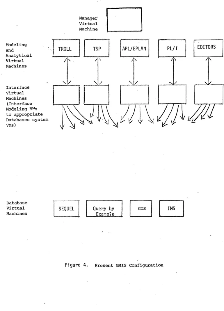
The configuration of virtual machines used in the present GMIS
is depicted in Figure 4, where each box denotes a separate virtual machine. The blocks across the top of the page represent different user-oriented programs (modeling and analytical systems, editors, etc.) and the blocks across the bottom of the page denote different data management systems, each
running on its own virtual machine. A user may access any modeling system and request a connection to any virtual machine. An interface virtual machine associated with the user's machine provides the necessary communi-cations interface between the user's analytical capability and the desired
database system. With this configuration it is possible for a user to
access the modeling or analytical capability with which he is most familiar, even though it may be running under an operating system different from the other available modeling or analytical apabilities. Thus, the user is not required to learn new analytical capabilities.
In addition, since each virtual machine may run any existing model
or program under its normal operating system, such a configuration eliminates the need to devote resources to translating application packages and programs between operating systems.
Furthermore, the GMIS configuration permits interaction between application languages and programs not originally envisioned by their developers.
For example, an analytical package is greatly enhanced by having its data management capabilities extended. Hence, a user of the APL/EPLAN
analytical capabilities, for example, may request data that is stored and managed by SEQUEL database management capabilities.
Manager Virtual Machine Modeling and Analytical Virtual Machines Interface Virtual Machines (Interface Modeling VMs to appropriate Databases system VMs ) Database Virtual Machines
SEQUEL Query by GIS IMS
l
lExample
4.4 GMIS Operation
A user of this system wishing a connection to another virtual machine sends a message to the virtual machine manager (depicted in Figure 4). The virtual machine manager will automatically log in an interface virtual machine. The interface virtual machine loads into its address space the appropriate programs which can transfer commands from the chosen modeling machine to the chosen database management machine and can tranfer data back
from the database management machine to the modeling machine. The user may then access the appropriate database machine, which waits for an "external
interrupt" to be initiated by the interface VM. The user, for example, may activate an APL model which could pass to the interface machine a SEQUEL command which could pass that command on to the SEQUEL database machine.
Figure 5 depicts a user console session that demraonstrates such an interaction. In Figure 5 the user has previously configured an APL/EPLAN machine connected to a SEQUEL machine. This example is taken from the early discussion of the resolution of Figure 1. Why did the average miles per gallon of cars sold per month go down? Note in Figure 5 the user is communicating with an APL virtual machine. The 'UERY' command is an APL function written for GMIS which sends the SEQUEL command to obtain Cadillac sales information
from the SEQUEL machine (via the interface VM). The SEQUEL machine returns the requested data in a vector 'VOLUME.'
To facilitate plotting, the user, from the APL machine, then converts the vector 'VOLUME' into a time series using the EPLAN function DF. The
Data
manage-ment
system )returns vector
Activate EPLAN
nbPdO2?iX2,,.1,.PAFP .)j.V.AIW£.P...
SAVED 13:45:59
06/02/75
Extract data on volume
of Cadillacs sold
M
p
A'SL tc!'CflL ULr8: Q. ),. )'t ODPL:
'D.,AC';.'CArVoLumv Change data to tme
*
~d~tXLL4~SA&~.~E
~OLUME
series for plotting
tUE 'Jt2t{ L qlA
tf2
r.a8Smila proedur
,, .
':~.PJI
$rE~t! VO1;tttf
";'t1!-~t"
P.A~,{ARt*
ttR
. loif :
Zt-,:
V
Z
t,
; '' .it . >...-"' '... , ' 2e . a,' .i .f, , '~, . ;*,:* ',....i,...,.. .~.~..:'.:.~..;.-...-,...: ....-.~....: u.~... ...--. ;.v ' >~*.7 >>...z2i:S:wS.6SF ... ...
I-O
1,31,C AF ___~
for Valiants
/( EPLANPlot
." ' ' F. .L 'C...: . .Fun
ction
I aOj
0,' / ' , ." o A- . .',, %. . I I I I I I I i I I 1 2 4 6 0 10 12 14.Tan-
r
A.$CL.'SA * I!? gA' R?Z: J'PO.; 1974 1 o a. AfnILA_,;i.:
* YAAZ, IJP,lAE.
Months
1,~~~~~~
Jan 75Plotting Cadillac and ..
ant sales
Figure 5: Using the Plotting Function for Reporting Data sG0C 0- oooo0000-' ,S . 0
3
0
o
30000- 20000- 1000 0-0user repeats this process to obtain data on sales volume of
Valiants. The user then activates the EPLAN PLOT function which
plots the sales volume of both Cadillacs and Valiants. (EPLAN [Schober, 1974] is an econometric modeling language consisting of a set of APL functions).
Note that the solid line in Figure 5 represents Valiant sales which appear to fall off during the energy crisis while the dotted line represents Cadillac
sales which appear to have remained constant. This gives evidence to
support a hypothesis discussed earlier in this paper which attempted to explain why average.miles per gallon of cars sold seemed to go down during the
"energy crisis." The hypothesis suggested that the affluent were buying big, luxurious cars while others in lower income levels were simply not buying cars at all.
The modeling and analytic systems which are presently active on the GMIS configuration are TROLL, EPLAN, TSP, PL/1, MPSX, BMDP, DYNAMO, STATPACK II, and APL. The database systems that are presently running are SEQUEL and Query by Example. The APL Data Language [IBM, 4] and VSAM
[IBM, 2] are presently being added.
4.5 Functions of the Virtual Machines 4.5.1 Functions of Manager Virtual Machine
The primary function of the manager virtual machine is to respond to user requests to create the connections between the virtual machines servicing that user. The other function of the manager is to disconnect and automatically log out the appropriate interface virtual machines once the user has logged out.
To accomplish these functions several procedures were added to the
user VM and the manager VM. When a user logs into his user machine he makes a request through his interface machine to connect to a database machine
by sending a message to the VM manager. The message is sent by calling a message sending routine:
CALL IXESEND (UMID, message_address, messagelength, messagecode)
The IXESEND procedure uses the VM/370 experimental inter-machine communi-cations facility, SPY [Hsieh 1974], for sending a message to the manager VM. The user initiated action causes the virtual machine manager to
receive an external interrupt. The external interrupt handlers which have been added to the manager VM perform the following: (a) check ID of sender 'UMID' for authorization; (b) look at the message located at 'message_address.' If the message is to log in an interface VM then it will check to see if such a VM is already running. If not, it
automatically logs one in (Note that the virtual machine manager has opera-tor privileges, which permit it to log in other virtual machines). The manager VM then sends a message to that interface machine for it to
load the appropriate interface module. The manager VM then sends a
complete code 'messagecode' to the user VM. If the message at 'message_ address' were a terminate message, the manager would automatically log off the user's interface VM. Furthermore, the manager periodically checks all interface VMs to see if they have "parents," i.e., if the user
VMs are currently logged in. If an interface VM does not have a parent, the manager VM automatically logs off the interface VM.
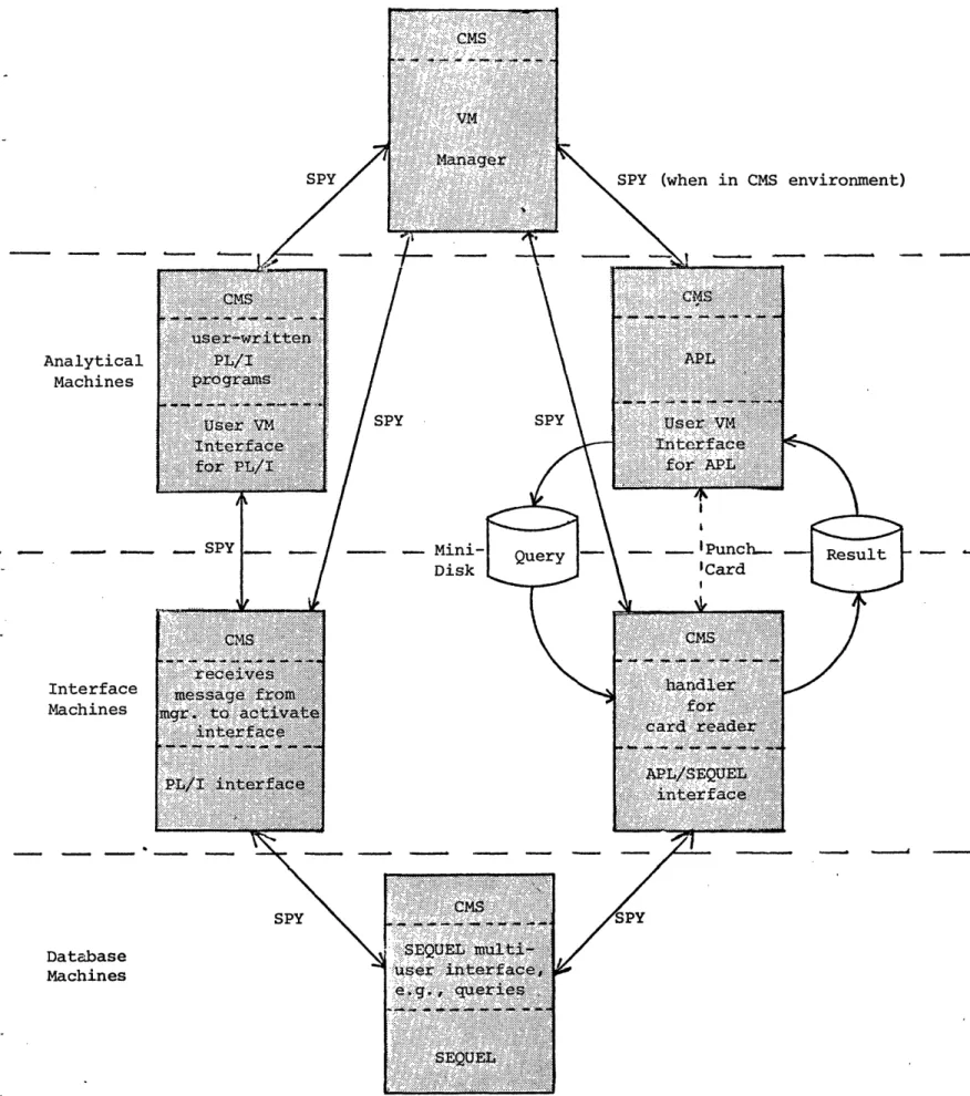
4.5.2 Functions of Interface Virtual Machines
The interface virtual machines provide mechanisms for user VMs to communicate with database VMs. When a user VM signals the manager VM to activate its interface'VM, this user VM also indicates in which modeling or analytical environment it is currently running, and to which database machine it wishes to send transactions. The manger VM uses
SPY (when in CMS environment)
Figure 6: Example of Communication Mechanisms Used Analytic Machine Interfai Machine' Database Machine.
routines. The user VM may then send a transaction to the interface VM by writing it to a CMS file and spooling a card from its virtual card punch to the interface VM's virtual card reader which generates an interrupt. The interface VM is alerted to the user's request by the interrupt, reads the transaction from the CMS file, reformats it for the SEQUEL database system, and sends the transaction to the SEQUEL VM via the SPY mechanism. After processing the transaction, the SEQUEL VM
I I
sends the reply to the interface VM via SPY again, the interface VM reformats the reply for APL, writes the reply to a CMS file, and signals the user VM running APL that the transaction is complete by spooling a
card to its virtual card reader. The user VM may now read the reply
from its CMS file and process it in any manner desired. This entire sequence is illustrated on the right hand side of Figure 6.
4.6 Communication Mechanisms between the Virtual Machines
j
The original philosophy of the VM concept was isolation [Donovan and Madnick 1975 ]. That is, each virtual machine should be unaware that other VMs exist. Until recently, applications of VM technologies were consistent with this philosophy. Fortunately, with respect to technologies needed for decision support systems, researchers have recently developed mechanisms to facilitate communication. These include: the page swap method and the data
move method Hsieh, 1974; Bagley et al., 1976]; segment sharing
[Gray 1975] ; channel-to-channel adaptor and virtual card punch and reader [Donovan and Jacoby 1975] available with standard release of VM/370
[IBM, 1 ]. The page swap method has been implemented by IBM using a VM enhancement of the IBM 370 DIAGNOSE instruction. This implementation, called "SPY," can be thought of as a "core-to-core" transfer between the two communicating
virtual machines. This is a very efficient mechanism for communicating between virtual machines. However, it requires the receiving VM to be capable of handling an external interrupt. Hence, this mechanism is best used between virtual machines running programs that can be modified to call external PL/I, FORTRAN or BAL routines, which would handle the interrupt and communications mechanisms. Under VM/370, the Conversational Monitor System (CMS) [IBM, 2] provides an operating system environment to modify, recompile and reload these programs for use in GMIS. The communication mechanisms used between the different classes of virtual
summarized here: machines in MIS as described in Section 45, are depicted in Figure 6 and/
- Between the User Analytical Facility and the VM Manager.
Since some modeling facilities would be difficult to modify to communicate directly with the Manager VM, a separate communication program which runs under CMS is invoked before the modeling facility is activated. This program sends the necessary messages to the Manager. The user may then activate a modeling facility under CMS or other operating systems.
- Between the modelling VM and the Interface VM. For PL/1, TSP, and other modeling facilities running under CMS, the communication to the interface machine is via "SPY" [Note we modified TSP to run under CMS]. However, for systems like APL and TROLL that run under their own environments, communication is via minidisks,
since standard versions of these systems have the
capa-bility of reading/writing disks, as well as punching and reading cards. The message is written on a shared minidisk. The inter-face VM is notified that such a message is waiting by punching a card on a virtual card reader. The interface VM reads that card and then reads the minidisk.
- Between the interface VM and a database VM. SPY"is used when the database VM is running in a CMS environment (e.g., in the case of SEQUEL and Query by Example). However, communication is via mini-disk, virtual card readers, and punches for data management systems
that do not run in a CMS environment (e.g., IMS in an OS/VSl environment). These communication facilities are explicitly shown in Figure 6 which depicts an example configuration of two analytical machines (user-written P1/I programs running under CMS and an APL environment running under CMS)
4.7 Functions of the Database Management Systems
The GMIS configuration has allowed the implementation of a data management capability which meets many of the requirements of Decision Support Systems outlined in Section 3.2.
GMIS provides the user with access to an interactive relational data management system, SEQUEL. This relational system has particular advantages for Decision Support Systems as it is able to provide a simple view of data. Policymakers and analysts have found that viewing data in the form of a table (relation) is conceptually simple. Further, as we have discussed in Section 2 (Characteristics of Decision Support Systems), the structure of the data, the ways a user will access it, and addition and deletion of data all change frequently in such applications. The relational system provides mechanisms for facilitating these changes; thus, there is no need to define a more complex data structure. The follow-on experimental system to SEQUEL which is called SYSTEM R [Astrahan et., 1976], holds even greater promise for use in decision support systems.
Although we have found that relational database systems are advantageous in certain public policy applications, most papers concerned with relational database technologies take their examples from inventory control areas or other non-shaded areas of Figure 3 [e.g., Date, 1975; Codd, 1970]. It is our feeling that applications like inventory control are areas where rela-tional systems appear to have little advantage. In fact, they may be at a disadvantage due to performance problems over traditional systems.
Decision support systems have requirements not only for data manipula-tion but for facilities for data analysis. Systems like TROLL, TSP, APL/EPLAN, are good data analysis facilities but have poor database facilities.
Facilities like SEQUEL, IMS, etc., have good database capabilities but poor analytical or statistical capabilities.
The implementation of database systems in the particular VM environ-ment of GMIS allows the enhanceenviron-ment of any data manageenviron-ment facility by
extending its analytical and statistical capabilities at minimal
cost. This enhancement is accomplished by running additional analytical systems which communicate with the database machine.
A common requirement of a decision support system is to allow multi-ple groups working on similar problems access to the same database. Each group may be familiar with a different analytical system. The data needed by all groups may be maintained by one group. The GMIS-type VM configura-tion allows multiple users (each using different analytical systems) to access the same data management system.
many data Another requirement of decision support systems resulted from the fact that/ series needed by the decision maker may be maintained in several different
data management systems, and there is often not time to transport these data series to a common data management system. The GMIS configuration allows multiple data management systems to exist simultaneously. Any user or analytical system can access data stored in a variety of data systems.
In decision support applications it is often desirable for different (and often incompatible) application programs (e.g., models) be able to interact with each other frequently. For example, there may exist an
States [e.g., MacAvoy and Pyndick, 1975]. At the same time, there may exist a regional demand model for energy by sector [e.g., Arthur D. Little, 1975]. If a decision maker wished to study supply and demand of natural gas in New England, it may be helpful to use these two models. The output of the first model (forecasted supply for the region) would be compared to the sum of output of the second model (demand by sector). Iterations of each model would then be performed until a balance occured. However, the first model is written in TROLL, which operates under its own operating system system and thus can not be run on the same system as the second model, which is written in FORTRAN, running under OS. By bringing these two models up on the GMIS configuration (where each could access data generated from the other), their interactions would be facilitated through
a common data management system. 4.8 Other Issues
We found the relational view of data particularly attractive to interactive public policy type applications. However, we recognize
both the experimental nature of these relational systems and the existence of many data series in more standard widely-used data management systems, e.g., IMS. Hence, we have provided for the availability of systems like IMS.
Additional advantages of the GMIS approach include increased
security among users of such a system. That is, security is improved over the more conventional method of operating different modeling capabilities
that were compatible in a multi-'programmed environment underneath the same operating system. This increased reliability of GMIS is discussed elsewhere (Donovan and Madnick,1975) and is an intuitive result of the fact that malicious or unintentional violations by the user must not only subvert the protection mechanisms of the operating system under
of the virtual machine monitor (VMM) if these violations are to affect another user. Hence, this hierarchical protection mechanism can provide much higher security. This concept is still somewhat controversial [Donovan and Madnick, 1976].
Since VM/370 software has been developed in such a way that each virtual machine can be accessed via a console, programs that were previously batch-oriented behave much as though they were inter-active. That is, a program can be created on line, edited, and submitted
for processing via a console.
Our experience with the GMIS approach in several application areas to date nas been very productive. The performance implications of this
configuration are discussed elsewhere (Donovan,1976). We feel that
further studies on cost benefit analysis and on increased effectiveness of users of this sort of system will quantitatively confirm our observations of the benefits of this approach.
5. NEW ENGLAND ENERGY MANAGEMENT INFORMATION SYSTEM (NEEMIS) EXAMPLE
APPLICATION
In this section we present an example to explicitly show the interaction necessary in a decision support system between a database system and an
analytical system. More importantly, this example was chosen to show that the computational capabilities advocated in this paper have a large
compara-tive advantage. 5.1 Purpose
This is a very detailed example. Its purpose is to show in a real setting the importance of:
(1) the interaction between an analytical system and a data manage-ment system, like that of GMIS;
(2) a flexible data management system for real decision support applications.
More specifically, this example shows:
(1) the amount of data manipulation required for validation;
(2) that queries had to be made to the data which were not originally planned for;
(3) that the interaction between an analytical capability and a database capability is frequent and is best accomplished in a user interactive mode;
(4) that other data series (not originally planned for) had to be introduced long after the study started;
(5) that an interactive analytical facility was helpful if not absolutely necessary for quickly responding to a problem; and
(6) in spite of the fact that the entire study was a complex one (requiring sophisticated data manipulation and complex analytical functions), the study was able to be accomplished in one week,
largely due to the fact that a computational facility (GMIS) with many of the features advocated in this paper was available.
5.2 New England Energy Mangement Information System
The example chosen here is taken from the New England Energy Manage-ment Information System (NEEMIS) Project Donovan and Keating, 1976] which
uses GMIS as its computational facility. The NEEMIS Project has been sponsored by the New England Regional Commission, and its primary focus is
on assisting the individual New England states and the overall region with energy policy decision making. The Project consists of four thrusts: making the
NEEMIS computational facility available to the states; maintaining relevant energy data series; maintaining energy-related computational models; and providing
a group of regional energy specialists accessible to regional policymakers. 5.3 Example Study within the NEEMIS Project
Let us explore the use of the GMIS computational capability in one [Donovan and Fischer, 1976].
recent study / One goal for the policymaker with respect to energy would be to increase the supply of petroleum or to reduce the demand for
petro-leum in the region. Since it is unlikely that oil would be discovered quickly in the New England region, if at all, considerable focus in the
region has been directed toward reducing demand and thus toward
conserva-tion efforts in energy. Residential space heating (home heating) consumes over 20 percent of all energy used in New England [Arthur D. Little 1975] and comprises over 10 percent of all energy consumed in the United States [Dole, 1975].
Oil is the source of over 70 percent of New England's home heat, and virtually all of this oil is imported into the region [Yankee Oil Man, 1974]. Hence, even a small reduction in home heating oil consumption could result in a considerable economic improvement in the region. The question for the policymaker is how can he affect reduction of consumption of fuel for home heating, using the handles over which he has some control, namely,
price and awareness (e.g., by raising the price of oil or by an advertisent campaign). To assist the decision-making process,the NEEMIS Project performed a
study to determine the relationship between price, awareness, and consumption. To establish this relationship consumption data was gathered using a sam-ple of homeowners in New England. Scott Oil Company made available delivery data, specifically, delivery data on 8000 individual homes within the suburban Boston area. The data is associated with the years from 1973 to 1975,
a period in which marked price changes, shortages, and behavioral changes occurred, hence, providing an opportunity to study the effects of these changes. The delivery data of the sample covers a period in which there were perhaps the greatest price changes in recent history (for instance, 1973/74 shows a 5 percent increase of price of oil to homeowners). It
was also a period in which awareness of energy use, shortages and expected price increases was great. Thus, the data affords an unusual opportunity
to calculate short-term elasticities. Weather data was gathered from 38 weather stations in New England. Additional data was gathered as it was needed.
Let us examine the computational steps that were required to calcu-late the short-term elasticity of consumption to price. That is, if the policymaker raises price by a certain amount, by how much could he expect consumption to be reduced? The purpose of this exercise is to give the reader some feeling for the operations needed in a decision support system.
To analyze consumption as a function of factors that vary over time, consumption per a regression model [Pindyck, 1976] was established that related change in / degree-day to a function of price and awareness. To normalize the effects of weather, consumption of households is expressed in gallons of oil con-sumed per degree-day (CPD). Degree-days are a weighted average of daily temperatures as they vary from a mean of 65 degrees. As price data was available on a monthly basis, we may write this expression as follows:
n
CPD A + Z A. X. m m
~
1 1 i=2The dependent variable (CPD ) is the average consumption per degree-day
ID
month of all consumers of the Scott Oil sample who received frequent
oil deliveries (five or morefeach season) during the three heating seasons. The independent variables (X2, X3) used in the model were price and
awareness. The price variable was set equal to the average price (in cents per gallon) of the oil company involved during the corresponding month (A1
is a constant term. A2 and A3 are coefficients of the independent variables). After much discussion the awareness variable chosen was the number of front-page headline columns of energy-related articles in the Thursday and Sunday
Boston Globe accumulated over the corresponding month. In this manner a monthly data series for this variable was compiled.
5.4 Computational Steps
The computational steps involved in developing the model and preparing the data were as follows; (1) validate the data;
(2) select the applicable data; (3) analyze the biases involved in such a selection; (4) make computations on the data for creating the dependent variable of the model; (5) run the model and introduce various mathematical alternatives to the model to improve its statistical properties; and
(6) use the most representative version of the model to compute the elasticities.
Because of the advantages of the computational facility chosen, all the above steps were accomplished and analyzed in less than one week.
5.4.1 Validate Data
In the first step the data had to be validated. The data was pro-vided by the oil company in such a form that associated with each customer was the amount of each delivery which that customer received in
the years 1972-1975. Many simple computations were performed on that data to check its validity. For example, for each customer, we added all deliveries in a year and compared them to the average yearly deliveries. Wide variations were examined more closely.
Note that while the computations were simple, often the types of accesses to the data were quite selective. Further, the number of accesses and tests was large. 5.4.2 Select Applicable Data
The second step was selecting the desired data. To use the proposed model it was necessary to have consumption data. This consumption data
was to be used to calculate CPD (the average monthly consumption per degree-m
day for the entire sample). However, using our source of
con-sumption data (namely, the oil company delivery records), concon-sumption can only be measured whenever a delivery occurs. Consumption in
a period is equal to the quantity delivered, where the period is defined as the time between this delivery and the previous one. Hence, those customers with frequent deliveries provide more reflective data on con-sumption, since consumption is monitored more often. For example, a cus-tomer who receives only one delivery during the heating season provides no information on the change of consumption during that heating season, whereas a customer who receives six deliveries provides a great deal of
information on the change in consumption during a heating season. Hence, data used to calculate the average consumption per degree-day per month were accessed by selecting only those customers with frequent oil deli-veries.
Note here is a query on the data that was not envisioned beforehand.
5.4.3 Analyze Biases
Taking a subsample from the entire sample that included only customers with frequent oil deliveries, introduces a problem for the policymaker, that is, biases. Therefore, it is necessary to make a bias analysis
(Step 3). To perform this analysis, we need to test the hypothesis that the subsample generated from step 2 has the same consumption habits as the sample as a whole. We may compare the consumption per degree-day averaged over an entire year (CPD ) for both the subsample and the entire sample to test this
Y
hypothesis. In order to do this in the analytical facility, a program was written that calculates consumption for the entire year by
summing all the deliveries made to an individual customer and dividing by the number of degree-days that occurred during that year. (Degree-day data is accessed from the database.) This is then done for all customers to get the average CPD . for each customer (i) and then averaged over all customers both in the entire sample and in the smaller sample giving CPDy
y for the subsample and for the sample. A statistical routine (written
in another language) is then invoked to perform statistical
tests to determine the significance of any differences if they exist. The analytical system was used to perform the calculations. The data manage-ment system was used to access the data by the criteria of all customers with frequent oil deliveries.
Note the interaction between the analytical system and the data management system.
5.4.4 Compute Dependent Variable
Step 4 involved the computation of the data used in the dependent variable CPD and in this step even more elaborate interaction between an
m
analytical facility and a database facility was necessary. The following procedure was used: (a) consumption for individual delivery periods was
calculated for each customer using delivery data; (b) consumption per degree-day for each customer for each delivery period was calculated by dividing the degree-days for each delivery period into the consumption of
that period; (c) the average consumption per degree-day for all customers CPDd for a particular day was obtained by averaging CPD for each customer
d
for that day; and finally, (d) the average consumption per degree-day for each day of a month CPD was calculated by summing CPD for each day of a
m
Note from a computational point of view (using Figure 4, GMIS) for substep (a), it was necessary to access the data associated with the
sub-sample for the amount of oil that was delivered during a period to each customer and for the dates of that period. For substep (b), it was necessary
to access the weather data to determine the number of degree-days in that same period. The calculation of CPD for a delivery period was performed
in the analytical system and then had to be stored back in the data manage-ment system. The computational aspects of substep (c) involved creating
365 individual pieces of data that correspond to the average consumption (over all of the customers) per degree-day for a particular day (CPDd). To compute CPDd one must access for a particular day each customer's
con-sumption per degree-day (as calculatedi.in substep (c)) and then sum CPD for a particular day over all customers and divide by the number
of customers to produce the resulting data series, CPDd (average consumption per degree-day for all customers for each day in the three heating seasons
under consideration). The computation involved in step (d) involved accessing this CPDd series and summing it for each day in a particular month, then
di-viding by the number of days in the month to obtain CPD .
m
Note that other data series, e.g, weather, had to be introduced, accessed, and used. Further, this entire step was accomplished in a matter of hours due to the interactive characteristics of the computational facility.
5.4.5 Run and Adjust Model
Step 5, the computation associated with running the model, involved activating a standard regression package that existed in our facility as the EPLAN package. In such a regression package one specifies the dependent
variables and all the independent variables. Data for those variables must be obtained from the data management system and passed back to the
analytical system where the regression is performed. The user receives output statistics as to the significance of each of the coefficients in
the regression, as well as overall statistics as to the goodness of the model.
2
The first such regression resulted in a relatively poor r statistic, and so a slight modification of the model was made. Specifically, it was felt that it would be more reflective to take the log of the awareness variable since the first article in a newspaper would have the most effect with each article in subsequent issues having less effect. After this modification was made the resulting statistics improved (that is, the r statistic as well as each of the coefficients). We then felt it would be more accurate to lag the awareness variable by one month, as perhaps a customer's reaction to the shortage situation would not occur until some time after this customer was made aware of the situation. Lagging
2
the awareness variable by one month again improved the r statistic as well as the significance of each of the coefficients.
It was then noted that the price data should be adjusted for inflation. Hence, another data series was established in the data management system, containing a set of inflation indicators for home heating fuel. The modeling system then used these standard inflation indicators to adjust the price data series. The model with the best statistics used adjusted prices, a lagging of awareness of by one peridd, and a log of awareness.
Note the comparative advantage that an interactive system gave in allowing for quickly interacting and changing the
model. Note yet another unexpected data series was introduced. Further, each new version of the model was made and examined in a matter of minutes.
5.4.6 Compute Elasticities
With respect to step 6, the result to the policymaker was the calcu-lation of the elasticity of price with respect to demand; an APL program was used. That program calculated the ratio of percentage change in price to percentage change in demand. The elasticity using the best model was -.15; that is, a 1% increase in price would produce a decrease in
consumption of .15%. This value of elasticity applies to the New England region and applies in the short term. A policymaker should be aware of this
important number.
The steps required to compute this elasticity further support the need for the close interaction of analytical capability and database
management systems, for a capability to be able to quickly incorporate new data series such as inflation indicators, to incorporate existing programs
such as those used in the bias analysis, and to incorporate different data series and access them at the same time (such as accessing the Scott Oil data series as well as weather data series supplied by the weather bureau).
Note that we were able to accomplish this entire
com-putation in under one week. That is not to say that others could not now duplicate that computation (now that the problem is defined, the data defined, etc.)in such a short
time using any number of computational facilities, but we do say that it would have been nearly impossible or very difficult
system due to the short time frame and the changing perception of the problem.
6. CONCLUSION
Common to many of the problems facing our country is the necessity to support decisions. Central to the process of supporting decisions is in-formation. Database system technology as it now stands lies at the heart of the technology necessary for decision support systems but is not adequate in itself for such systems. Decision support systems, as has been shown in this work, are different from the traditional management and operational control systems to which database systems have been successfully applied in the past. The differences are due primarily to the problems being ad-dressed by decision support systems. That is, the nature of these problems is such that they are constantly changing, the data needed to solve them is not always known, solutions to these problems are needed in a short timeframe, and attention must be given to the cost of developing solutions
and other software in decision to these problems. Our experience in using database systems, analytical systems / support systems for energy-related areas (the NEEMIS work discussed in this
article) and other private and public sector areas only further confirms our realization of the inadequacies of existing database management systems and technologies as far as the needs of decision support systems are con-cerned. We have used an approach as explained here that alleviates
some of the deficiencies of traditional database systems. By developing a framework in which different database systems and different analytical and modeling systems may be integrated together within the same system, the
transfer costs and time loss that would necessarily be involved in inte-grating existing programs and existing data series to solve a particular


![Figure 3: Framework for Management Information System From [Gorry and Scott Morton, 1971]](https://thumb-eu.123doks.com/thumbv2/123doknet/14540812.535391/17.940.48.860.73.1080/figure-framework-management-information-gorry-scott-morton.webp)