HAL Id: cea-02481249
https://hal-cea.archives-ouvertes.fr/cea-02481249
Submitted on 5 Mar 2020
HAL is a multi-disciplinary open access
archive for the deposit and dissemination of
sci-entific research documents, whether they are
pub-lished or not. The documents may come from
teaching and research institutions in France or
abroad, or from public or private research centers.
L’archive ouverte pluridisciplinaire HAL, est
destinée au dépôt et à la diffusion de documents
scientifiques de niveau recherche, publiés ou non,
émanant des établissements d’enseignement et de
recherche français ou étrangers, des laboratoires
publics ou privés.
Resonant optical transduction for photoacoustic
detection
Thomas Lauwers, Alain Glière, Skandar Basrour
To cite this version:
Thomas Lauwers, Alain Glière, Skandar Basrour. Resonant optical transduction for photoacoustic
detection. SPIE Photonics West 2020 - Optoelectronics, photonic materials and devices, Feb 2020,
San Francisco, United States. �cea-02481249�
Resonant optical transduction for photoacoustic detection
T. Lauwers*
a, A. Glière
a, S. Basrour
ba
Université Grenobles Alpes, CEA, LETI, F38000 Grenoble, France;
bUniversité Grenobles Alpes,
CNRS, Grenoble INP, TIMA, 38000 Grenoble, France
ABSTRACT
A highly sensitive optical transduction system suitable for photoacoustic trace gas detection is presented. The system includes a thin deformable hinged cantilever assembled on an optical fiber to form a Fabry-Perot cavity, whose length varies according to the acoustic pressure disturbance. Consequently, the optical power of the reflected light fluctuates at acoustic frequencies around the working point, which is stabilized to prevent from environmental drift of the interference fringes. The resonant mechanical structure proposed in this study shows a spectral response in good agreement with FEM simulation, good linearity and stability, with a noise equivalent pressure of 12 µPa/√Hz.
Keywords: Fiber-optic Fabry-Perot, photoacoustic sensor, optical transduction, acoustic sensor, hinged cantilever
microphone
1. INTRODUCTION
Optical transduction methods are useful for remote detection in harsh environments where electronics may be damaged by high temperature or sensitive to electromagnetic noise for example. In the field of acoustics, optical transductions are indeed a very sensitive solution for some applications such as photoacoustic detection ([1], [2]), acoustic noise measurement and ultrasound detection, in gaseous or liquid environment.
A wide range of optical sensors has been developed for acoustic measurement and can be found in the literature, based on fiber coupling [3], fiber Bragg grating [4] or classical interferometric systems like Mach-Zehnder [5] or Michelson [6] interferometer. The Fabry-Perot (FP) interferometer is also of great interest, with high sensitivities and reduced dimension, especially in the case of fiber tip FP sensors where the sensing element is placed directly at the end of an optical fiber. Due to the cylindrical symmetry of the system, circular membranes are often preferred for the sensitive element. Several materials have been proposed, like silver [7], graphene [8] or parylene [9], with a noise equivalent pressure ranging from 33 µPa/√Hz to 83 µPa/√Hz in the audible frequency range. Chen et al. [10] proposed recently a stainless steel cantilever resonator well adapted to fiber tip FP acoustic sensor, with higher sensitivities due to the free end of the cantilever and reaching a noise equivalent pressure of 8 µPa/√Hz at a frequency of 1 kHz.
In this paper, we present a new geometry, based on a resonant hinged cantilever, suitable for acoustic detection in the kHz range, with high sensitivity and easy to install. The acoustic sensor will shortly be placed into a photoacoustic cell usable for the detection of gas traces.
2. DESCRIPTION AND DESIGN OF THE SENSITIVE PART
2.1 Description of the transducer
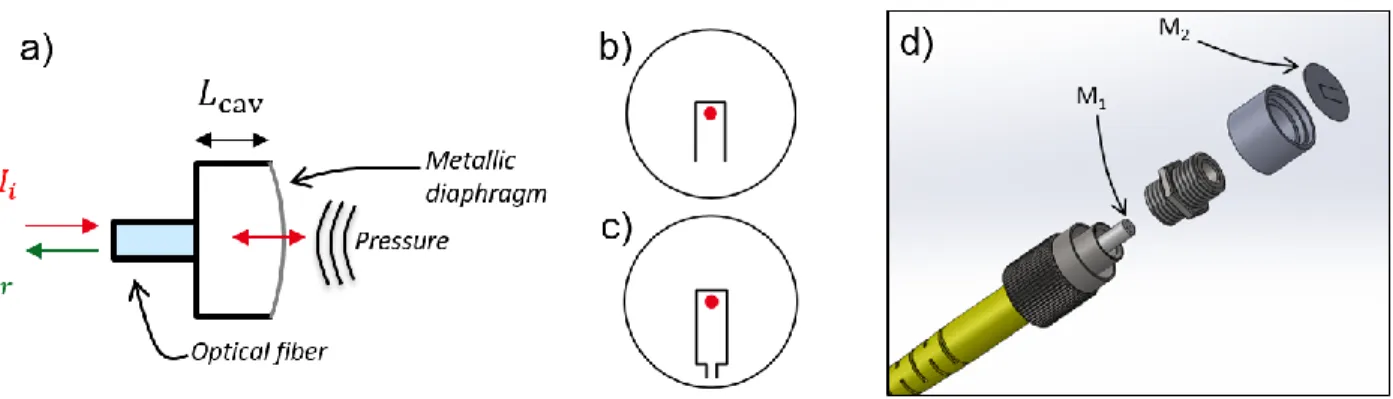
The FP cavity is composed of two mirrors (Figure 1a,d): the first one (M1) corresponds to the fiber endface while the end mirror (M2) is a reflective membrane, designed to be sensitive to weak acoustic perturbations. The optical fiber is screwed on a mechanical cylinder that supports the thin membrane and forms the interferometric cavity. A probe laser light is injected in the optical fiber and a photodetector converts the reflected light into a measurable electric signal, proportional to the acoustic perturbation.
Figure 1. Schematic of the fiber tip FP sensor (a), the designed membranes (b, c) and 3D view of the fiber system (d). Red dots indicate the location of the probe laser spot. M1 depicts the first fiber/air interface, M2 the stainless-steel mirror and Lcav the FP cavity length.
In order to enhance the displacement caused by the acoustic wave, a cantilever beam is shaped on the membrane, resulting in a coupled mechanical structure, combining the circular plate and the cantilever dynamics (Figure 1b). The free end of the cantilever is located at the center of the membrane, so that a maximum displacement of the structure is probed by the laser, indicated by the red dot on the figure. However, to reach a resonance frequency in the kHz range, either a very thin membrane or a long cantilever is needed. A new geometry, consisting in a hinged cantilever beam, is thus proposed here (Figure 1c). As the hinge considerably decreases the fundamental resonance frequency of the cantilever, this geometry simultaneously allows an easier micromachining of the membrane (40 µm thickness) and a millimetric length cantilever. The ventilation slit, corresponding to the gap between the cantilever frame and the rest of the membrane, must be chosen as thin as possible in order to maximize its acoustic resistance and thus the pressure differential existing between the two sides of the cantilever.
The FP cavity length 𝐿cav influences both the optical sensitivity and the acoustic behavior of the sensor. On the one hand,
a thin cavity reduces the optical losses, which increases the contrast of the interference pattern and thus enhances the optical sensitivity. However, a too small value of the cavity length causes a large interfringe period, which may be not covered by the laser wavelength tunability range. On the other hand, on the acoustic side, given the ventilation slit, a thick cavity favors an increase of the differential pressure at the working frequency and thus of the mechanical displacement. However if the cavity length is too large, the static pressure or unwanted low frequency pressure variation will not equilibrate on both sides of the membrane, causing an important instability of the optical fringes. Finally, the optical cavity length is chosen as large as possible while keeping a reasonable interference contrast.
In the following sections, a detailed study is presented for the two configurations: the plain clamped-free cantilever (Figure 1b) and the hinged cantilever (Figure 1c).
2.2 Mechanical structure and coupling with acoustics
In the configuration showed above, the cantilever is shaped directly on the membrane and no additional element is added to the mechanical structure. Using a single layer of material greatly simplifies the assembly and reduces the fabrication steps but gives rise to another difficulty, that is the mechanical coupling between the plate and cantilever dynamics, which complicates the design of the system. To describe how the coupled system behaves, a first approach consists in considering the two isolated structures and to calculate analytically the fundamental resonance frequency of the simple clamped-free beam using the Euler-Bernouilli theory and the clamped circular plate using the Kirchhoff-Love theory:
𝑓0,beam= 𝛼CF 2𝜋 𝑡 𝐿2√ 𝐸 12𝜌 and 𝑓0,plate= αplate 2𝜋 𝑡 𝑅2√ 𝐸 12𝜌(1 − 𝜈2) (1)
Where 𝑓0,beam (resp. 𝑓0,plate) denotes the resonance frequency of the first mode of a clamped-free beam (resp. clamped
circular plate), 𝛼𝐶𝐹= 3.52 and αplate = 10.22 are the coefficient corresponding to the fundamental mode of resonance, 𝑡
modulus and 𝜈 the Poisson coefficient. In order to represent analytically the dynamics of the two samples (Figure 1b,c), it is useful to consider the reduced frequency, defined as the ratio between the two resonance frequencies:
𝑓red= 𝑓0,beam 𝑓0,plate = 𝛼CF 𝛼plate √1 − 𝜈2× (𝑅 𝐿) 2 (2) If 𝑓red> 1, the fundamental mode of the plate will be at a lower frequency and will disturb the beam dynamics. Thus, we
want to design the sensor in the regime where 𝑓red< 1 in order to decouple the plate and beam dynamics. To approximate
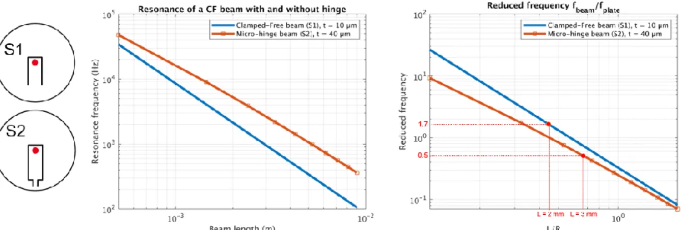
the coupled structure to a cantilever, the condition 𝐿/𝑅 ≫ 1 is needed, which is not achievable with the geometry of Figure 1b. One way to avoid the unwanted plate resonance is to design a hinge on the cantilever on a thicker structure. This shifts the first resonance of the plate to higher frequencies while keeping the resonance of the cantilever at the same frequency. We show in Figure 2 the resonance frequency and reduced frequency of the two samples introduced in Figure 1b,c. The first sample (S1) is a cantilever beam of 2 mm x 1 mm shaped on a 10 µm thick circular plate with a diameter of 9 mm. The second one (S2) is a 3 mm x 1 mm hinged cantilever beam cut on a 40 µm thick plate with the same diameter. The hinge consists of an extension of the beam of 100 µm x 200 µm. The hinged cantilever resonance is calculated with a Finite Element Method (FEM) model on a 2D shell structure (COMSOL Multiphysics, COMSOL AB, Sweden). An eigenmode resolution is performed. As can be seen on the resonance frequency plot (Figure 2 left), the fundamental resonance of the cantilevers are close, around 2 kHz for S1 and 2.5 kHz for S2. On the right, we can see that the geometry leads to coupled resonance for the 10 µm case (𝑓red= 1.7), while the 40 µm plate resonates at higher frequencies without
any perturbation on the beam dynamics (𝑓red= 0.5).
Figure 2. On the left, evolution of the resonance frequency with the length of the beam. On the right, reduced frequency versus L/R is plotted. The analytical frequency of the 10 µm thick cantilever (S1) is plotted in blue and the numerical frequency of the 40 µm thick hinged cantilever (S2) is plotted in red.
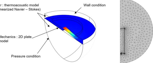
To obtain a precise prediction of the hinged cantilever behavior, a FEM simulation has been performed that takes in account the complete membrane geometry and the coupling between mechanic and acoustic phenomena. We can see on Figure 3 a 3D view with two different physical domains modeled: the white volume corresponds to the acoustic domain, while the colored surface corresponds to the mechanical domain, which separates the acoustic domain in two parts linked by the ventilation slit (FP cavity above and external environment below).
The mechanical domain has been modeled by a 2D shell with a perfectly clamped boundary condition on its circular external limit. The high aspect ratio of the membrane (𝑅/𝑡 ~ 100) lies in the domain of validity of the shell theory. The acoustic domain has been modeled by a thermoacoustic model, involving the linearized Navier-Stokes equations system. This model has been chosen because some characteristic lengthscales of the domain (ventilation slit and membrane thickness) are of the same order as the acoustic boundary layers. The ventilation is fixed to the minimum size allowed by laser cutting (50 µm).
Figure 3. On the left, 3D view of the simulated system. The colormap displayed on the membrane corresponds to the mechanical displacement at the cantilever resonance frequency. On the right, mesh of the 2D plate.
To simulate the acoustic response of the transducer, a harmonic pressure condition is applied on the external surface of the hemispheric domain situated below the shell. This boundary condition simulates an incoming plane wave because the domain size is smaller than the typical acoustic wavelength considered in the simulation (𝜆𝑎𝑐> 10 cm at 2 kHz). Above
the shell the optical cavity is closed with wall boundaries (no slip and isothermal condition). The system is solved for different frequencies and the cantilever maximum displacement is calculated. The transfer function, expressed in nm/Pa, is compared to the experimental result in section 4.2.
2.3 Optical readout
The optical intensity reflected from the Fabry-Perot cavity is written 𝐼𝑟= 𝐼𝑖× 𝑅FP, where 𝐼𝑖 is the incident power and 𝑅FP
the reflectivity obtained for a two light-beam interferometer:
𝑅FP(𝜆, 𝐿cav) = 𝑅1+ 𝑅2+ 2√𝑅1𝑅2cos (
4𝜋𝐿cav𝑛
𝜆 ) (3)
𝑅1,2 are the reflectivities of the fiber endface and the membrane, 𝑛 the index of the medium (in our case 𝑛 = 1). In this
model, the reflectivity is a function of the optical cavity length 𝐿cav and the laser wavelength 𝜆. In the presence of an
acoustic perturbation 𝑝, the cavity length oscillates at the acoustic angular frequency 𝜔𝑎𝑐 with an amplitude 𝛿𝐿(𝑝). This
cavity length modulation affects the reflected intensity 𝐼𝑟(𝑝) = 𝐼𝑟+ 𝛿𝐼𝑟:
𝛿𝐼𝑟(𝑝) = 𝐼𝑖
𝑑𝑅FP
𝑑𝐿 𝛿𝐿(𝑝) sin (𝜔𝑎𝑐𝑡) (4) A way to maximize this signal is to have a working point fixed to the maximum of the derivative, called quadrature point Q (see Figure 6). For long measurements, the working point shifts, because de FP cavity is sensitive to environmental factors like temperature or humidity. The solution is to work in a closed-loop system, where the working point Q follows the fringe drift (this closed-loop system is detailed in [11]).
2.4 Sensor sensitivity
From the previous sections, we can define an optical sensitivity in mV/nm. This quantity corresponds to the voltage variation measured by the photodetector for a given displacement 𝛿𝐿:
𝑆mV/nm= 𝐺𝑃𝐷𝐼𝑖[ 𝑑𝑅FP 𝑑𝐿 ]𝑄 = 𝑉𝑄 𝑅𝐹𝑃(𝑄) [𝑑𝑅FP 𝑑𝐿 ]𝑄 (5) Where 𝐺𝑃𝐷 denotes the photodetector gain in V/W, 𝑉𝑄 the DC voltage measured at the working point from the reflected
Using the analytical formula for the reflectivity we can easily calculate the derivative and find: 𝑆mV/nm= 𝑉𝑄 𝑅1+ 𝑅2 (8𝜋𝑛 𝜆 ) √𝑅1𝑅2 (6)
The mechanical sensitivity has been calculated numerically with FEM simulation, and corresponds to the displacement at the center of the membrane given an incident acoustic pressure 𝑝:
𝑆nm/Pa=
𝑑𝐿
𝑑𝑝(𝜔𝑎𝑐) (7)
Where 𝜔𝑎𝑐 is the acoustic angular frequency. The final sensor sensitivity can be written 𝑆mV/Pa= 𝑆mV/nm× 𝑆nm/Pa,
leading to the linear sensor relation:
𝑉(𝑝) = 𝑆mV/Pa× 𝑝 (8)
3. FABRICATION
The membrane is processed by laser cutting on a thin stainless steel film. The two main difficulties of the micro fabrication of the cantilever beam are the thermal dissipation during the process and the minimal spot size achievable by the laser:
- Thermal dissipation has been reduced with the use of a heat sink and an optimized laser cut path. The use of thicker films also increases the thermal inertia and reduces the risk of residual strain on the final structure. - The minimal size achievable is limited by the wavelength of the laser. For the Nd:YAG laser used (Cielle, Tau
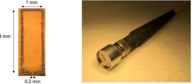
Tech), the spot size has a diameter of 35 µm, leading to a minimal cutting size ranging from 50 µm to 100 µm. This limitation causes a decrease of the mechanical sensitivity of the structure. The ventilation size chosen for the sample shown on Figure 4 left is of 50 µm, which is close to the spot laser size and thus generates an irregular laser cut.
The membrane support is realized in aluminum, with a controlled optical cavity length and a SMA fiber thread for direct mechanical alignment (see Figure 4). The membrane is glued to the support with a UV glue, which has the advantage of curing quickly when exposed to UV light.
Figure 4. On the left, microscope view of the 3 mm x 1 mm cantilever beam with the 100 µm x 200 µm hinge (bottom). On the right, membrane assembled on the SMA optical fiber.
4. EXPERIMENTAL RESULTS
4.1 Description of the experiment
To test the hinged cantilever frequency response and sensitivity, an acoustic experimental bench was installed (Figure 5). The light from a laser diode (Toptica, model DL pro) propagates through an optical fiber towards the sensor, and the reflected light is retrieved from the third port of an optical circulator. A photodetector (Femto, model OE-200) measures the light intensity variation with a large bandwidth (500 kHz). A lock-in amplifier (Zurich Instrument, model HF2LI) is used for both the acoustic excitation on a calibrated speaker at the resonance frequency 𝑓res and the demodulation of the
optical signal at the same frequency (AC channel). The DC channel is employed to control that the working point stays at the quadrature point, where the maximum slope of the interference fringe is obtained.
Figure 5. Diagram of the acoustic calibration setup. Optical fibers are drawn in green, electric connections in black.
4.2 Sensor characterization
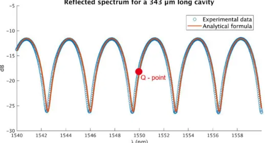
The first step of the sensor characterization consists in the measurement of the optical sensitivity. For this purpose, a wavelength scan is carried out to obtain the experimental Fabry-Perot reflectivity. As shown on equation 3, the cavity length 𝐿cav fixes the interfringe period while the two reflectivities 𝑅1,2 fix the offset and the contrast of the reflected optical
fringes. Figure 6 shows the experimental optical response and the fitted analytical model.
For this sample, we calculate a cavity length of 343 µm, 𝑅1= 2.45 % and 𝑅2= 1.15 %. 𝑅1 is identified to be the
reflectivity of the fiber endface and 𝑅2 the effective reflectivity of the membrane mirror. By knowing the refractive index
of the fiber core we obtain a theoretical reflectivity of 3.3 % at 1.55 µm, which is slightly higher than the experimental reflectivity. This difference can be easily explained by the fact that the fiber end used has not been cleaved. The second mirror experimental effective reflectivity is very low with respect to the expected theoretical reflectivity. This is due to the optical loss of the optical cavity which can be explained by several factors, namely the loss of the optical cavity originating from the fiber divergence, the imperfect shape of the second mirror and the lack of precise alignment.
Figure 6. FP interference fringes for the hinged cantilever beam with a 343 µm long cavity. Reflected power is referenced with respect to incident light in port 2.
The second step is to stabilize the Q-point at the maximum slope of the fringes (DC reflected signal at Q-point 𝑉𝑄 = 160 mV) and to make the acoustic measurement. A frequency sweep is performed to locate the resonant frequency
which is found to be 2040 Hz. An acoustic calibration is then made at 2040 Hz (Figure 7 on the left), giving an acoustic sensitivity of 𝑆mV/Pa = 117 mV/Pa. The comparison of the simulation sensitivity in nm/Pa and the experimental
sensitivity in mV/Pa is made with the normalization using the optical sensitivity given in equation 6.
Figure 7. On the left, calibration measurement of the acoustic sensor (measured data is plotted in red and linear fit in continuous blue line). On the right, transverse beam displacement in nm/Pa evaluated at the laser spot location for different acoustic frequencies with an integration time of 1s. The blue curve corresponds to the simulation result and the red curve corresponds to the experimental measurement normalized by the fitted optical sensitivity 𝑆mV/nm.
The Figure 7 (right) compares the measured and calculated frequency response of the hinged cantilever, with a 4 % error on the predicted resonance frequency but an experimental displacement of 65 nm/Pa which is half that of the simulated displacement.
The measured amplitude loss and resonance shift can come from the assembly of the membrane on the support (stiffness of the glue and uneven distribution of the glue on the edges of the membrane). Most importantly, the quality of the laser cutting can cause geometrical variations of the cantilever. The ventilation slit size has been chosen as small as possible i.e. with the same order of magnitude as the marking laser spot size, which led to defects on the cut path, especially in the region close to the hinge (Figure 4 left). These defects, as well as the imperfect clamping due the glue characteristics and dispense, are not taken into account in the numerical model and could explain the differences between the simulation and the experiment.
The measured noise standard deviation at resonance frequency is equal to 𝜎 = 1.44 μV/√Hz. Using the calibrated sensitivity of 117 mV/Pa, we find a Noise Equivalent Pressure (NEP) of 12 µPa/√Hz at 2040 Hz. Due to the imperfection of the insulation box, it is difficult to dissociate the white noise coming from the laboratory environment from the sensor's own noise. This, as well as the inaccuracies of the membrane cut-out, leads to a NEP slightly higher than expected but still close to that of the state of the art fiber tip FP acoustic sensors [10]. Nevertheless, the new geometry proposed here offers many advantages in terms of simplicity of fabrication and assembly.
5. CONCLUSION AND PERSPECTIVES
We have proposed in this paper a new membrane geometry for fiber tip Fabry-Perot acoustic sensor, based on a hinged cantilever beam fabricated by laser micromachining technique. The cantilever has the dimension of 3 mm x 1 mm, cut on a stainless steel circular membrane with a diameter of 9 mm and a thickness of 40 µm. The hinge is an extension of the beam and measures 100 µm x 200 µm. We showed that, with this geometry, it is possible to obtain a high sensitivity and to uncouple the beam and the plate dynamics. Moreover, the significant thickness of the plate allows an easy handling and gluing of the membrane on the support, as well as a reduction of the thermal strain during the cutting process.
The measured frequency response is in good agreement with the FEM simulation and the transducer shows a good linearity and a high sensitivity, with a NEP of 12 µPa/√Hz at resonance.
A more compact system is being developed, with improved fabrication process, higher sensitivity and the use of a current-controlled DFB laser for a finer closed-loop control. This system will then be integrated in a photoacoustic sensor for trace gas detection.
REFERENCES
[1] G. Wissmeyer, M. A. Pleitez, A. Rosenthal, and V. Ntziachristos, ‘Looking at sound: optoacoustics with all-optical ultrasound detection’, Light: Science & Applications, vol. 7, no. 1, Dec. 2018, doi: 10.1038/s41377-018-0036-7. [2] T. Kuusela and J. Kauppinen, ‘Photoacoustic Gas Analysis Using Interferometric Cantilever Microphone’, Applied
Spectroscopy Reviews, vol. 42, no. 5, pp. 443–474, Sep. 2007, doi: 10.1080/00102200701421755.
[3] S. Dass and R. Jha, ‘Micro-tip Cantilever as Low Frequency Microphone’, Scientific Reports, vol. 8, no. 1, Dec. 2018, doi: 10.1038/s41598-018-31062-9.
[4] C. Li, X. Peng, J. Liu, C. Wang, S. Fan, and S. Cao, ‘D-Shaped Fiber Bragg Grating Ultrasonic Hydrophone With Enhanced Sensitivity and Bandwidth’, Journal of Lightwave Technology, vol. 37, no. 9, pp. 2100–2108, May 2019, doi: 10.1109/JLT.2019.2898233.
[5] D. Gallego and H. Lamela, ‘High-sensitivity ultrasound interferometric single-mode polymer optical fiber sensors for biomedical applications’, Opt. Lett., vol. 34, no. 12, p. 1807, Jun. 2009, doi: 10.1364/OL.34.001807.
[6] M. J. Murray, A. Davis, and B. Redding, ‘Fiber-Wrapped Mandrel Microphone for Low-Noise Acoustic Measurements’, Journal of Lightwave Technology, vol. 36, no. 16, pp. 3205–3210, Aug. 2018, doi: 10.1109/JLT.2018.2838051.
[7] B. Liu, J. Lin, H. Liu, A. Jin, and P. Jin, ‘Extrinsic Fabry-Perot fiber acoustic pressure sensor based on large-area silver diaphragm’, Microelectronic Engineering, vol. 166, pp. 50–54, Dec. 2016, doi: 10.1016/j.mee.2016.09.005.
[8] C. Li, X. Gao, T. Guo, J. Xiao, S. Fan, and W. Jin, ‘Analyzing the applicability of miniature ultra-high sensitivity Fabry–Perot acoustic sensor using a nanothick graphene diaphragm’, Meas. Sci. Technol., vol. 26, no. 8, p. 085101, Aug. 2015, doi: 10.1088/0957-0233/26/8/085101.
[9] Z. Gong, X. Zhou, K. Chen, X. Zhou, and Q. Yu, ‘Parylene-C diaphragm-based fiber-optic Fabry-Perot acoustic sensor for trace gas detection’, in 2017 International Conference on Optical Instruments and Technology: Advanced
Optical Sensors and Applications, Beijing, China, 2018, p. 5, doi: 10.1117/12.2286076.
[10] K. Chen, Q. Yu, Z. Gong, M. Guo, and C. Qu, ‘Ultra-high sensitive fiber-optic Fabry-Perot cantilever enhanced resonant photoacoustic spectroscopy’, Sensors and Actuators B: Chemical, vol. 268, pp. 205–209, Sep. 2018, doi: 10.1016/j.snb.2018.04.123.
[11] X. Mao, S. Yuan, P. Zheng, and X. Wang, ‘Stabilized Fiber-Optic Fabry–Perot Acoustic Sensor Based on Improved Wavelength Tuning Technique’, Journal of Lightwave Technology, vol. 35, no. 11, pp. 2311–2314, Jun. 2017, doi: 10.1109/JLT.2017.2651151.