A simple, flexible and generic deterministic approach to uncertainty quantifications in non linear problems: application to fluid flow problems
Texte intégral
Figure
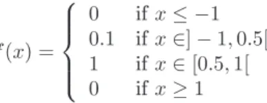
![Figure 1: Error in the ev aluation of Ψ(U ∞ ) when U ∞ ∈ ] 1 4 , 1 2 [ and U ∞ ∈ ] 1 2 , 3 4 [ for optimal meshes.](https://thumb-eu.123doks.com/thumbv2/123doknet/12744438.358087/12.918.291.603.474.695/figure-error-ev-aluation-ψ-u-optimal-meshes.webp)


Documents relatifs
This last step does NOT require that all indicator be converted - best if only a small percent need to be reacted to make the change visible.. Note the
Keywords: Backtesting; capital allocation; coherence; diversification; elicitability; expected shortfall; expectile; forecasts; probability integral transform (PIT); risk measure;
We define a partition of the set of integers k in the range [1, m−1] prime to m into two or three subsets, where one subset consists of those integers k which are < m/2,
When the vector field Z is holomorphic the real vector fields X and Y (cf. This follows from a straightforward computation in local coordinates.. Restriction to the
Any 1-connected projective plane like manifold of dimension 4 is homeomor- phic to the complex projective plane by Freedman’s homeomorphism classification of simply connected
Cauchy-Pompeiu formula (this is a generalization, published by Pompeiu in 1905, of the classical Cauchy formula from 1825).. What are the
• How does the proposed algorithm behave if the t faulty processes can exhibit a malicious behavior. ⋆ a malicious process can disseminate wrong
While it is well known that database vendors typically implement custom extensions of SQL that are not part of the ISO Standard, it is reasonable to expect statements that use
