HAL Id: hal-03006336
https://hal.archives-ouvertes.fr/hal-03006336
Preprint submitted on 15 Nov 2020
HAL is a multi-disciplinary open access
archive for the deposit and dissemination of
sci-entific research documents, whether they are
pub-lished or not. The documents may come from
teaching and research institutions in France or
abroad, or from public or private research centers.
L’archive ouverte pluridisciplinaire HAL, est
destinée au dépôt et à la diffusion de documents
scientifiques de niveau recherche, publiés ou non,
émanant des établissements d’enseignement et de
recherche français ou étrangers, des laboratoires
publics ou privés.
Jon Legarreta, Laurent Petit, François Rheault, Guillaume Theaud, Carl
Lemaire, Maxime Descoteaux, Pierre-Marc Jodoin
To cite this version:
Jon Legarreta, Laurent Petit, François Rheault, Guillaume Theaud, Carl Lemaire, et al.. Tractography
filtering using autoencoders.. 2020. �hal-03006336�
PREPRINT. PAPER UNDER REVIEW
Jon Haitz Legarreta
Sherbrooke Connectivity Imaging Laboratory (SCIL) Videos & Images Theory and Analytics Laboratory (VITAL)
Department of Computer Science Université de Sherbrooke, Canada
Laurent Petit
Groupe d’Imagerie Neurofonctionnelle (GIN) Univ. Bordeaux, CNRS, CEA, IMN, UMR 5293, France
François Rheault
Sherbrooke Connectivity Imaging Laboratory (SCIL) Department of Computer Science
Université de Sherbrooke, Canada
Guillaume Theaud
Sherbrooke Connectivity Imaging Laboratory (SCIL) Department of Computer Science
Université de Sherbrooke, Canada
Carl Lemaire Centre de Calcul Scientifique Université de Sherbrooke, Canada
Maxime Descoteaux*
Sherbrooke Connectivity Imaging Laboratory (SCIL) Department of Computer Science
Université de Sherbrooke, Canada
Pierre-Marc Jodoin*
Videos & Images Theory and Analytics Laboratory (VITAL) Department of Computer Science
Université de Sherbrooke, Canada
*Co-senior author. These authors contributed equally.
October 9, 2020
A
BSTRACTCurrent brain white matter fiber tracking techniques show a number of problems, including: generating large proportions of streamlines that do not accurately describe the underlying anatomy; extracting streamlines that are not supported by the underlying diffusion signal; and under-representing some fiber populations, among others. In this paper, we describe a novel unsupervised learning method to filter streamlines from diffusion MRI tractography, and hence, to obtain more reliable tractograms. We show that a convolutional neural network autoencoder provides a straightforward and elegant way to learn a robust representation of brain streamlines, which can be used to filter undesired samples with a nearest neighbor algorithm. Our method, dubbed FINTA (Filtering in Tractography using Autoencoders) comes with several key advantages: training does not need labeled data, as it uses raw tractograms, it is fast and easily reproducible, it does not rely on the input diffusion MRI data, and thus, does not suffer from domain adaptation issues. We demonstrate the ability of FINTA to discriminate between “plausible” and “implausible” streamlines as well as to recover individual streamline group instances from a raw tractogram, from both synthetic and real human brain diffusion
MRI tractography data, including partial tractograms. Results reveal that FINTA has a superior filtering performance compared to state-of-the-art methods.
Together, this work brings forward a new deep learning framework in tractography based on autoen-coders, and shows how it can be applied for filtering purposes. It sets the foundations for opening up new prospects towards more accurate and robust tractometry and connectivity diffusion MRI analyses, which may ultimately lead to improve the imaging of the white matter anatomy.
Keywords Representation Learning · Autoencoder · diffusion MRI · Tractography · Filtering
1
Introduction
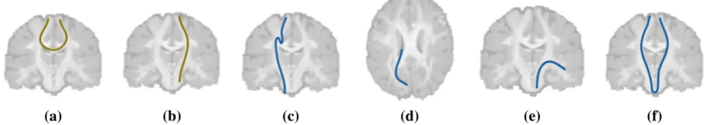
Tractography is a diffusion Magnetic Resonance Imaging (dMRI) data feature extraction technique that provides information about the brain white matter structural connectivity. These connectivity pathways are composed of streamlines virtually representing fascicles of white matter fibers. Tractography methods face a number of challenges when propagating streamlines, including avoiding the early termination of the tracking procedure (Smith et al., 2012; Girard et al., 2014), providing streamlines between gray matter regions that are known to be connected while avoiding spurious streamlines, ensuring the full occupancy of the white matter volume by the streamlines (Rheault et al., 2019), and a complete gray matter surface coverage when streamlines reach the cortex (St-Onge et al., 2018). As a result, and despite the efforts to address these issues, white matter tracking procedures are known to produce a disproportionately large amount of invalid streamlines (referred to as “implausible”s in this work, as opposed to “plausible” streamlines). The category of invalid streamlines spans a broad group of streamlines that are known not to satisfy accepted anatomical constraints. These include streamlines that contain loops or sharp bends; streamlines that stop in non-white matter tissues, such as the cerebrospinal fluid (CSF); streamlines that prematurely stop in the white matter; or streamlines describing trajectories between gray matter regions that are not connected structurally. An illustration of “plausible” and “implausible” streamlines can be seen in figure 1. According to the ISMRM 2015 Tractography Challenge benchmark (Maier-Hein et al., 2017), tracking methods produce a non-negligible proportion of invalid streamlines as a trade-off between sensitivity and specificity. The study reported that non-existing, false positive connections were present in as many as 64% of the submissions. Hence, improved filtering strategies are required to detect and remove anatomically unfeasible streamlines and mitigate the undesired drifts of the streamline propagation methods.
(a) (b) (c) (d) (e) (f)
Figure 1: Schematic representation of “plausible” and “implausible” streamlines: (a) “plausible” streamlines belonging to the corpus callosum; (b) “plausible” streamlines belonging to the corticospinal tract; (c) “implausible” streamline containing a loop or a sharp bend; (d) “implausible” streamline stopped at the cerebrospinal fluid; (e) “implausible” streamline stopped in the white matter (or hitting a white matter or atlas boundary); (f): “implausible” streamline describing an invalid bundle.
Filtering “implausible” streamlines generated by tracking methods is a necessary step to avoid biologically unrealistic connectivity patterns and biases in reconstructing the brain structural connectome from diffusion MRI data (Sotiropoulos and Zalesky, 2019; Yeh et al., 2019) (see section 1.1.1). The quality of the tractograms influence various aspects of the connectome analysis, including the connectivity density, the clustering degree or the existence of connections themselves, among others (Yeh et al., 2016). Hence, tractogram filtering, in its various forms, is essential towards providing a reliable imaging evidence using diffusion MRI of how the white matter fascicles are arranged in the brain. Filtering in tractography can also be regarded as a procedure that separates streamlines that are useful to serve a certain task from those that are not. As such, some filtering methods involve a clustering operation which may be used to extract a predefined set of bundles (see section 1.1.2). While connectomics applications (Sotiropoulos and Zalesky, 2019) require every anatomically “plausible” fiber to be recovered, other applications often need a more specialized set of fibers. For example, in the human versus macaque study by Takemura et al. (2017), only streamlines from the occipital white matter are considered. In Chenot et al. (2019) only fibers from the pyramidal tract are retained, while in Bullock et al. (2019) the brain fibers connecting the dorsal and ventral posterior cortex are the ones of interest.
Streamline filtering can be seen as an application of choice for deep learning classification methods. Unfortunately, neural networks are not easily applicable to brain tractography, mostly because of the fundamental difficulty of building a labeled dataset. In fact, finding irreproachable ground truth streamlines is a very difficult endeavour, with significant differences in reproducibility measures even among well-trained expert neuroanatomists, as shown in Rheault et al. (2020a). Also, depending on the task at hand, the labeling of the streamlines might vary considerably, and hence may require time-consuming manual verification and/or relabeling. Classification neural networks are trained to predict a fixed number of classes, and thus cannot be used to predict a different set of classes without being retrained on a newly labeled set of data.
This work proposes a deep autoencoder for streamline-based tractography filtering. The method, named FINTA (Filtering in Tractography using Autoencoders), is trained on non-curated, raw tractograms. Once training is over, the learned latent space is a low-dimensional representation of the input streamlines where similar streamlines are located next to each other. The filtering process is then carried out by projecting to the latent space examples of reference streamlines. Then, the to-be-filtered streamlines are projected to the latent space and labeled according to a nearest neighbor test. We demonstrate the filtering ability of FINTA on both synthetic and human brain datasets. Additional quantitative evaluations show its superior performance compared to both anatomy-based tractography filtering methods and the state-of-the-art RecoBundles (Garyfallidis et al., 2018; Rheault, 2020) streamline similarity filtering method. Similarly, FINTA is linear in terms of the streamline count at test time, allowing for a faster tractogram filtering.
1.1 Related work
1.1.1 Filtering plausible versus implausible streamlines
Diffusion MRI tractography methods generate tractograms that may contain several million candidate streamlines representing white matter fiber populations. Yet, a large proportion of such streamlines are anatomically “implausible”, meaning that they do not comply with neuroanatomical constraints attributed to fiber populations. A regular tractogram including only anatomically “plausible” streamlines can contain in the order of 500 000 to 3 000 000 streamlines (Presseau et al., 2015). Hence, having an automatic procedure to filter out “implausible” streamlines is critical. Tractography filtering is currently approached based on five main patterns: (i) streamline geometry features; (ii) region-of-interest-driven streamline inclusion and exclusion; (iii) clustering; (iv) connectivity-based; and (v) diffusion signal mapping or forward models (Jeurissen et al., 2019; Sotiropoulos and Zalesky, 2019; Jörgens et al., 2020). The first category of criteria is based on anatomical features of individual streamlines, such as unfeasible streamline length or local curvature indices. Streamline inclusion and exclusion criteria incorporate white matter and/or tissue local and connectivity constraints for streamline traversal (Schilling et al., 2020). Such principles are usually concatenated into a sequence of restrictions to form a succession of step-wise refinement rules (Maier-Hein et al., 2017; Sarubbo et al., 2019; Jeurissen et al., 2019; Jörgens et al., 2020). Clustering approaches, such as QuickBundles (Garyfallidis et al., 2012), use a similarity measure to remove non-meaningful data issued by a tracking method. These methods are based on the assumption that a properly defined distance measure is able to split apart the relevant streamlines from the rest. These methods usually require a representative set of streamlines of the population that is being studied to be built so that they can be used as reference models to exclude the extraneous streamlines. Connectivity-based approaches, such as the one presented by Wang et al. (2018), propose to remove undesired streamlines usually imposing some regularization constraint on the tractogram-derived connectivity matrices. The forward models, such as SIFT/SIFT2 (Smith et al., 2013, 2015), LiFE (Pestilli et al., 2014) and COMMIT/COMMIT2 (Daducci et al., 2015; Schiavi et al., 2020), posit that only a subset of streamlines in a whole-brain tractogram are essential or relevant to explain the underlying diffusion signal. SIFT/SIFT2 is based on modifying the local fiber Orientation Distribution Function (fODF) based on the diffusion signal, whereas LiFE and COMMIT/COMMIT2 use specific local models to weigh the contribution of the signal to the streamline representation. Anatomical a priori constraints can be incorporated to improve the accuracy of the reconstructed pathways. Some of these methods have large computational demands in terms of the time required to filter the tractogram of a single subject (in the order of hours) (O’Donnell et al., 2019).
A number of works use deep learning-based methods for tractography filtering. de Lucena (2018) used an autoencoder to learn features about the input tractogram, and then used a residual network to regress on those features. However, their results were only limited to the uncinate fascicle and no comparison to other filtering methods was provided. More recently Astolfi et al. (2020) proposed a geometrical deep learning method to filter tractograms. The method implements a supervised geometric model which builds on streamline graph structures.
1.1.2 Streamline clustering
White matter streamline clustering (also referred to as bundling) allows to assign every streamline in a tractogram to the bundle it belongs to (O’Donnell and Westin, 2007; Maddah et al., 2008; Li et al., 2010; Wassermann et al., 2010; Guevara et al., 2011; Garyfallidis et al., 2012; Jin et al., 2014; Wassermann et al., 2016; Siless et al., 2018; Sharmin
et al., 2018; Garyfallidis et al., 2018). It is a procedure where the streamlines of interest need to be identified from the rest of the streamlines (the rejection class). The task of attributing a streamline to a bundle needs to address the fundamental question of how streamlines are similar to, or different from, each other. One of the challenges lies in finding the appropriate measure to quantify the affinity of streamlines, the other major difficulty being computing such affinities or distances in a reasonable time.
Probabilistic model-based methods (e.g. Dayan et al. (2018)) or traditional machine learning-based frameworks (e.g. Brun et al. (2004); Wang and Shi (2018); Kumar et al. (2019); Bertò et al. (2020)) have also been proposed to solve the clustering task. However, some of the findings in these works are limited to clustering a single bundle, require separate learning models for each bundle, are still affected by the streamline-wise distance computational complexity, or suffer from the trade-off of the granularity of the arrangement.
A number of different strategies have been developed recently to address the streamline clustering task using deep learning networks, including stacked, bi-directional siamese networks (FS2Net) (Patil et al., 2017), regular convolutional neural networks using different streamline re-parameterizations (FiberNet/FiberNet2.0) (Gupta et al., 2017, 2018), or custom feature vectors (TRAFIC) (Lam et al., 2018), (DeepWMA) (Zhang et al., 2020), ensemble models using fully connected neural networks (Ugurlu et al., 2018), or representation learning methods (Zhong et al., 2020) based on recurrent autoencoders. Yet, many of these methods still work in a supervised fashion, and thus do not allow to generalize to a variable number of classes, require a distinctly trained network for each bundle, or present results limited to a reduced number of bundles.
As opposed to the previous deep learning approaches, a few other ones (Wasserthal et al. (2018); Pomiecko et al. (2019); Li et al. (2020)) provide voxel-wise segmentations representing the locations traversed by a given bundle’s streamlines. Most of these approaches are based on a U-Net (Ronneberger et al., 2015) or another form of classification convolutional neural network using a specialized feature vector or parameterization. The major drawback of voxel-based bundle segmentation methods is the need of a separate model (including the need to train it) for each bundle, and hence, a variable number of models depending on the target classes.
In this work, we describe a novel unsupervised learning framework based on deep autoencoders to filter streamlines in diffusion MRI tractography. We demonstrate its performance on both synthetic and in vivo human brain tractography data, including partial tractograms. We provide evidence that the described deep learning setting can be applied to filter “plausible” and “implausible” streamlines as well as to multi-label classification problems without requiring to be retrained.
2
Material and methods
Autoencoders (AEs) are deep neural networks that have the ability to learn an efficient representation of the data in an unsupervised fashion using a dimensionality reduction approach (Hinton and Salakhutdinov, 2006). AEs are trained to reconstruct an input signal through a series of compressing operations (known as the encoder) followed by a series of decompression operations (referred to as the decoder). As shown in figure 2, between the encoder and the decoder is the so-called latent space, where each point is an encoded representation of an input data sample. In this work, the input data is a streamline, which is a sequence of three-dimensional points. A streamline is an ordered sequence of
points s = {c1, c2, . . . , cns}, ci ∈ R
3that represents a package of similarly oriented fibers and describing a neural
pathway within the brain white matter. A tractogram representing a set of M streamlines is mathematically expressed
as T = {s1, s2, . . . , sM}.
AEs have two major advantages over other types of neural networks. First, they are trained on raw unlabeled data, which is a major asset in the context of brain tractography. Second, since the latent representation is obtained by a series of compressing operations, two neighboring points in the latent space correspond to input data instances that share similar characteristics (Painchaud et al., 2019). Thus, the encoded representation can be used to redefine the notion of inter-data distance. In the context of tractography, instead of measuring the distance between two streamlines with a geometric distance function as is usually the case (Siless et al., 2013), one can project the streamlines into the latent space and measure their Euclidean distance.
Our filtering approach, shown in figure 2, can be summarized by the following steps: 1. Train an autoencoder with a large, raw, uncurated tractogram.
2. From the training tractogram, label the streamlines of interest. These streamlines could be examples of anatomically “plausible” fibers, streamlines representing fibers belonging to predefined sets of bundles, or any sorts of streamlines that are of interest for some application. These streamlines are labeled as positive streamlines.
3. Project the positive streamlines into the latent space with the encoder network. The positive latent vectors are illustrated by the golden circles in figure 2. Note that in case of more than two classes (as for a multi-label bundling operation) streamlines of several classes could also be projected into the latent space.
4. Given a new tractogram that ought to be filtered, project its streamlines into the latent space (cf. the three bold circles in figure 2(b)) and label it according to the distance to its nearest neighbor.
(a)
(b)
Figure 2: Schematic representation of tractography filtering with FINTA: (a) training time; (b) test time. Although 1D convolutions are used in the proposed framework, convolutional blocks are depicted using a 2D shape for illustrative purposes.
The proposed AE is a fully convolutional neural network whose overall structure is summarized in table 1. Our convolutional AE accepts a streamline at its input. Since raw streamlines have a different number of vertices (long streamlines have more vertices than shorter ones), we re-sample the streamlines so that they all have an equal number of 256 vertices. The latent space length was fixed at a value of 32 for all of our experiments.
The autoencoder was trained with an Adam optimizer (Kingma and Ba, 2015) with a mean squared-error loss. The hyper-parameters were adjusted using a Bayesian search method. The learning rate of the optimizer was fixed to a value
Table 1: FINTA autoencoder structure. The encoder uses strides of size 2, and the decoder uses strides of size 1. The decoder’s upsampling stages use an upsampling factor of 2. The autoencoder uses ReLU activations throughout its convolutional layers.
Part Type Features Size
input - - 3; 256 encoder 1D conv 32 256 1D conv 64 128 1D conv 128 64 1D conv 256 32 1D conv 512 16 1D conv 1024 8
latent space fully connected 32
decoder upsampling + 1D conv 1024 8 upsampling + 1D conv 512 16 upsampling + 1D conv 256 32 upsampling + 1D conv 128 64 upsampling + 1D conv 64 128 upsampling + 1D conv 32 256 output - - 3; 256 2.1 Data
Experiments were carried out using the “Fiber Cup” synthetic data (Fillard et al., 2011; Côté et al., 2013), the ISMRM 2015 Tractography Challenge human-based synthetic dataset (Maier-Hein et al., 2015), as well as the BIL&GIN in vivo human subject brain dataset (Mazoyer et al., 2016; Chenot et al., 2019).
2.1.1 “Fiber Cup” synthetic data
A synthetic dataset re-generated (using Fiberfox (Neher et al., 2014)) from the “Fiber Cup” phantom (Fillard et al., 2011; Côté et al., 2013) was used as a simplified test set mimicking the human brain white matter bundle anatomy. The “Fiber Cup” phantom contains 7 bundles, and the ground truth consists of a total of 7833 streamlines. The raw diffusion
data were generated using 30 gradient directions, a diffusion gradient strength of 1000s/mm2, and a 3mm isotropic
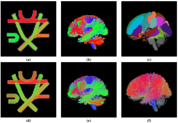
spatial resolution for a 64 × 64 × 3 volume. Figure 3(a) shows the ground truth tractogram for the synthetic “Fiber Cup” phantom.
2.1.2 ISMRM 2015 Tractography Challenge human-based synthetic data
The ISMRM 2015 Tractography Challenge dataset of Maier-Hein et al. (2015) was used in a further step towards a more complex and realistic scenario. The dataset consists of a clinical-style, realistic single subject tractogram (approximately 200 000 ground truth streamlines) with 25 ground truth fiber bundles, raw diffusion-weighted data and a structural T1-weighted MRI volume generated using Fiberfox (Neher et al., 2014). The raw dMRI data were generated at a 2mm
isotropic spatial resolution, with 32 gradient directions, and a b-value of 1000s/mm2. Figure 3(b) shows the sagittal
left view of the ground truth tractogram for the ISMRM 2015 Tractography Challenge dataset.
2.1.3 Human data
A sample of 39 subjects of the BIL&GIN (Brain Imaging of Lateralization by the Groupe d’Imagerie Neurofonctionnelle) human brain dataset (Mazoyer et al., 2016; Chenot et al., 2019) was used to gauge the performance of FINTA. Acquisitions were done with a Philips Achieva 3 Tesla MR scanner using 21 non-colinear diffusion gradient directions
and a diffusion gradient encoding strength of 1000s/mm2with four averages and an isotropic spatial resolution of
2mm. In this work, only the corpus callosum was considered, and within the bundle, homotopic streamlines lying within any of 26 pairs of gyral-based segments were considered as “plausible” streamlines. Additional details about the gyral-based callosal segments used for the extraction of the streamlines, shown in figure 3(c), are provided in section A.5.
(a) (b) (c)
(d) (e) (f)
Figure 3: Tractograms corresponding to the considered datasets. Upper row: (a) ground truth tractogram from the “Fiber Cup” dataset; (b) ground truth tractogram from the ISMRM 2015 Tractography Challenge dataset; (c) sagittal left view of the gyrus-wise homotopic callosal streamline models corresponding to the BIL&GIN dataset. Lower row: test sets corresponding to the tracking performed on each of the three datasets: (d) view of the “Fiber Cup” test set containing 4963 streamlines; (e) sagittal left view of ISMRM 2015 Tractography Challenge test set containing 63615 streamlines; (f) sagittal left view of a randomly picked test subject corresponding to the BIL&GIN dataset and containing 55160 streamlines.
3
Experimental
The same experiment design was implemented for the three datasets. Noise-free diffusion data were used for the “Fiber Cup” and ISMRM 2015 Tractography Challenge datasets, and no denoising procedure was required for the BIL&GIN dataset. A Constrained Spherical Deconvolution (CSD) (Tournier et al., 2007) method using a spherical harmonics order of 6 was used to extract the fiber ODFs from the raw dMRI data. The probabilistic setting of the Particle Filtering
Tracking(PFT) method by Girard et al. (2014) using white matter seeding and whole brain tracking were employed
for the “Fiber Cup” and the ISMRM 2015 Tractography Challenge datasets to generate the sets for the autoencoder. The extracted streamlines were processed and scored according to the procedure in Maier-Hein et al. (2017) to obtain the “(anatomically) implausible streamline” and “(anatomically) plausible streamline” sets. For the ISMRM 2015 Tractography Challenge dataset, the anterior commissure (CA) and the posterior commissure (CP) bundles were left out of the experiments since the tracking algorithm was unable to extract them or the extracted bundles did not meet the scoring system criteria. Hence, 23 bundles were used in the experiments.
As a result of this procedure, the “implausible” sets on the “Fiber Cup” and ISMRM 2015 Tractography Challenge datasets were comprised of streamlines that did not reach the cortical surface (or the corresponding terminal regions in the “Fiber Cup”), streamlines whose trajectories described sharp bends, and streamlines connecting regions that were not actually connected in the ground truth (see examples of such trajectories in figure 1).
The probabilistic setting of the PFT method was likewise used for the BIL&GIN human brain dataset. The resulting tractograms were registered (Avants et al., 2011) to the MNI template common space using the MNI152 2009 standard-space T1-weighted average structural 1mm isotropic resolution template image (Fonov et al., 2011). For the experiments
in this work, only the callosal subset of the generated tractograms was used. The “plausible” streamlines within this subset consisted of the streamlines within 26 gyral-based homotopic callosal segment pairs (see section A.5 for further details about their definition). The “implausible” set comprised, as for the “Fiber Cup” and ISMRM 2015 Tractography Challenge datasets, streamlines that did not reach the cortical surface, describing sharp bends, having a single endpoint in the callosal region, having endpoints in non-white matter tissues, or connecting both hemispheres through non-callosal segments or tissues (e.g. the brainstem). The procedure was supervised by a neuroanatomist. The procedure yielded, on average, 41838 streamlines per-subject (standard deviation: 5648) for the considered callosal dataset. The lower row in figure 3 shows the test set tractograms, including both “plausible” and “implausible” streamlines, corresponding to all three datasets.
The ratio of “implausible” streamlines over the resulting tractograms was in-line with the findings in previous studies: 79% for the “Fiber Cup” dataset (similar to the figures reported by Côté et al. (2013) for probabilistic methods); 46% for the ISMRM 2015 Tractography Challenge dataset (see the valid connection ratios across submissions reported in Maier-Hein et al. (2017)); and 89% on average (standard deviation: 2%) for the callosal BIL&GIN dataset. All streamlines were resampled to contain an equal number of points (256) and their endpoints were aligned for each dataset. The obtained streamlines were split randomly into training/validation and test sets using an 80%/20% ratio. The proposed convolutional autoencoder was trained in an unsupervised manner using the training split of both the “plausible” and “implausible” streamlines issued by the probabilistic tracking methods. The filtering threshold was set by finding the optimal point in the receiver operating characteristic (ROC) curves evenly rewarding true positives and penalizing false positives.
3.1 Comparison to other filtering methods
The quantitative comparison was performed on the callosal BIL&GIN dataset. FINTA was compared to both anatomy-based tractography filtering methods and two variants (single-bundle and multi-bundle) of RecoBundles (Garyfallidis et al., 2018; Rheault, 2020), a state-of-the-art method applicable to partial data. The anatomy-based filtering methods were applied successively, each one filtering the previous step’s output, as used in several works such as Maier-Hein et al. (2017); Sarubbo et al. (2019). The purpose of including the results of each step of this filtering pipeline (baseline filtering methods #1 to #4) was to show the successive improvement of the classification performance scores by using anatomical heuristics. The models of “plausible” streamlines used for the RecoBundles experiments were built according to Rheault (2020), and based on the 26 gyral-based homotopic callosal segment pairs (see section A.5). The multi-bundle RecoBundles experiment considered each gyrus-wise homotopic callosal streamline model as a separate, parameterizable entity, whereas the single-bundle RecoBundles method considered their concatenation as a single target group. This yielded a total of 6 tractography filtering methods as baselines:
1. filtering based on streamline length (named length within this text); 2. filtering with loop removal (no_loops);
3. filtering with early stops in cerebrospinal fluid (no_end_in_csf ); 4. filtering with early stops in the white matter (end_in_atlas); 5. single-bundle RecoBundles (recobundles_single);
6. multi-bundle RecoBundles (recobundles_multi).
To estimate the ability of the methods to preserve the underlying anatomy in terms of the gyrus-wise callosal streamline homotopic connections kept by the predicted positives, a valid gyrus-wise homotopic callosal streamline group count (shortened as VGW for the sake of compactness) rate was computed as the average ratio of the preserved streamline groups to the existing ones. The streamlines were recovered from the positives predicted by each method using the anatomical criteria defined for each segment. To estimate the task performance uniquely, a success rate (SR) measure was computed as the unweighted average of the classification measures and the valid gyrus-wise homotopic callosal streamline group count rate.
3.2 Time requirements
The filtering clock time of FINTA was measured on each of the datasets. For quantitative comparison purposes, tractograms of different sizes were generated from the ISMRM 2015 Tractography Challenge data using the same procedure described earlier. In total, six (6) different tractograms were generated containing 20 000, 40 000, 100 000, 200 000, 600 000, and 1 000 000 streamlines, respectively. The time required to filter each of these tractograms was measured for both FINTA and RecoBundles three (3) times, and the mean and standard deviation values were computed for each tractogram and method. In all cases, solely the time required for filtering was measured, excluding I/O
operation time. All time tests were performed on a conventional desktop machine (Intel(R) Xeon(R) W-2133 CPU @ 3.60GHz 6 core processor; 16 GB RAM; NVIDIA GeForce GTX 1080 Ti 12 GB graphics card).
4
Results
4.1 Tractogram latent space
The autoencoder’s latent space allows to re-interpret the streamline pair-wise distance. For illustrative purposes, a number of randomly picked “plausible” streamlines were assigned to their corresponding bundle (or gyrus-wise homotopic callosal streamline group for BIL&GIN), and together with some “implausible” streamlines, they were projected into the latent space of a trained autoencoder. Figure 4 shows a view of the latent spaces corresponding to each of the three datasets. The views were generated by applying a t-SNE dimensionality reduction (van der Maaten and Hinton, 2008) to the autoencoder’s latent space vectors. The figure suggests that streamlines belonging to the same bundle (or streamline group) lie at a short distance from each other whereas “implausible” streamlines are uniformly distributed. Similarly, it provides evidence supporting that the autoencoder setting can be generalized and give way to multi-label streamline classification tasks such as bundling.
(a) (b) (c)
Figure 4: Latent space views using a t-SNE dimensionality reduction. (a) “Fiber Cup” data; (b) ISMRM 2015 Tractography Challenge data; (c) Callosal BIL&GIN human brain data. The number of projected streamlines was limited in each case for visualization purposes. The callosal BIL&GIN data corresponds to a randomly picked subject which was missing all streamlines in 8 of the gyral-based segments.
Furthermore, the application of mathematical tools in the latent space is straightforward. Figure 5(a) shows the interpolation principle applied to the latent space. Interpolating in the latent space allows to explore the space through a series of intermediate representations between any number of input streamlines of choice. Figure 5(b) and (c) show streamlines interpolated in the latent space between streamline pairs corresponding to two distinct sets of bundles of the “Fiber Cup” dataset. This example stresses the underlying significance of the latent space streamline pair-wise distance. Our proposed algorithm relies on the underlying hypothesis that the Euclidean distance between the latent representation of two streamlines is a good proxy to measure their structural similarity. Thus, the fact that a linear interpolation between two latent vectors leads to a smooth transition between their reconstructed streamlines underlines that the learn manifolds are smooth and that the latent Euclidean distance is a good similarity metric.
The reconstruction of the streamlines at the output of the autoencoder involves decoding the samples in the latent space. Section A.1 shows the reconstructed tractograms corresponding to the “Fiber Cup” test set streamlines.
(a)
(b) (c)
Figure 5: Latent space interpolation. (a) Schematic representation of latent space streamlines interpolation. The streamline representation in the latent space allows to choose a pair of encoded streamlines and fill the space between them through a series of interpolated streamlines. (b) and (c) “Fiber Cup” latent space streamline interpolation: streamlines interpolated between the instances at the boundaries of each series: (b) bundles 1 and 5; (c) bundles 4 and 7 (see the bundle numbering in Côté et al. (2013)). Only the structural shapes of the bundles used for the interpolation are shown for the sake of clearness. The streamlines are shown with a larger diameter with respect to the one used for the rest of the figures.
4.2 “Fiber Cup” synthetic data
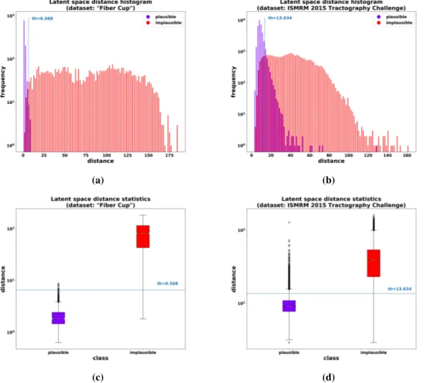
Figure 6 (a) and (c) show the nearest neighbor latent space distance distribution histograms and within-class mean and variance for the “Fiber Cup” dataset. The figure illustrates the filtering principle of FINTA based on the boundary between the inliers and outliers: the “plausible” streamline within-class nearest neighbor distance is low (close to 0 for the “Fiber Cup”) and shows a reduced variance. As a contrast, the “implausible” streamlines show a much higher mean distance to their nearest neighbor streamline, as well as a higher variance. Note that the distance measure is computed considering the “plausible” streamlines from the train set as the reference.
(a) (b)
(c) (d)
Figure 6: Nearest neighbor latent space distance distribution: histogram (a) and within-class mean and variance (c) corresponding to the “Fiber Cup” dataset test set streamlines; histogram (b) and within-class mean and variance (d) corresponding to the ISMRM 2015 Tractography Challenge. The dashed lines indicate the filtering threshold distance in each case. Note that the vertical axes are in logarithmic scale.
As quantitatively shown in table 2, the filtering distance threshold obtained by means of the autoencoder-based strategy allows to filter out the undesired “implausible” streamlines with a high degree of success.
Table 2: Filtering performance for the “Fiber Cup” and the ISMRM 2015 Tractography Challenge datasets.
Measure Dataset
“Fiber Cup” ISMRM 2015 Tractography Challenge
Accuracy 0.99 0.91
Sensitivity 0.99 0.91
Precision 0.97 0.91
F1-score 0.98 0.91
The predicted positive streamlines for the “Fiber Cup” are shown in figure 7. These are the streamlines considered as “plausible”s by FINTA from the test set, and hence include both the true positives and the false positives. Quali-tatively, looking at the tractogram bundle color code information, and in agreement with the quantitative results, the “implausible”s seem to have been substantially filtered out, implying a decreased influence of the false positives.
Figure 7: Predicted positives on the test set corresponding to the “Fiber Cup” dataset. Note that, in contrast to the input dataset shown in figure 3(d), the filtered tractogram shows a bundle color code information that matches better the “Fiber Cup” ground truth shown in figure 3(a), implying that “implausible” streamlines have been eliminated to a large
extent.
(a) (b)
Figure 8: False positive and false negative streamlines issued by FINTA on the “Fiber Cup” dataset test set. (a) false positives: streamlines labeled as “plausible”s by FINTA but considered “implausible”s by the scoring method; (b) false negatives: streamlines labeled as being “implausible” by FINTA but considered “plausible”s by the scoring method.
Figures 8(a) and (b) show, respectively, the false positive and false negative streamlines as detected by FINTA for the “Fiber Cup” dataset, and color-coded according to the latent space nearest neighbor distance. From the figures and the corresponding highlighted areas it can be drawn that, at least for part of the streamlines, FINTA has identified that these streamlines were misclassified in the reference set: in figure 8(a) a large part of the highlighted streamlines seem to be close to an anatomically “plausible” streamline within the bundle at issue. Many of these false positives are labeled so because they end 1 or 2 voxels away from the terminal regions (which would correspond to the cortical surface or gray matter border on human subject brain data). Conversely, part of the highlighted streamlines in figure 8(b) describe
trajectories that could have been identified as anatomically “implausible” due to erratic bends. This illustrates how close from the ground truth our results are.
FINTA takes around 0.2s to filter the “Fiber Cup” test tractogram.
4.3 ISMRM 2015 Tractography Challenge human-based synthetic data
The nearest neighbor latent space distance distribution histograms and within-class mean and variance for the ISMRM 2015 Tractography Challenge dataset are shown in figure 6(b) and (d). As it is the case with the “Fiber Cup” dataset, although a larger degree of overlap between classes is observed, our autoencoder-based filtering strategy allows to obtain a threshold to filter out the undesired “implausible” streamlines with a degree of success of approximately 91% over all measures (see table 2). Here again, the latent space similarity metric shows the same behavior in both experiments: “implausible” streamlines have a larger distance to the reference nearest neighbor.
For qualitative visualization purposes, figure 9 shows the streamline-wise classification tractograms for some selected cases corresponding to the ISMRM 2015 Tractography Challenge dataset test set, color-coded according to their nearest neighbor distance in the latent space. In particular, “plausible” predictions corresponding to the the corticospinal tract (CST) and the optic radiation (OR) bundles are shown, together with an example corresponding to “implausible” streamlines. As it can be drawn from the scale bar, the latent space dissimilarity distances for the true positive samples (a) to (f) are below the distance threshold determined shown in figure 6(b, d) (13.634) while the distances for the “implausible” predictions shown are above that threshold. The filtered whole brain tractogram is shown in A.2.
(a) (b) (c)
(d) (e) (f)
(g) (h) (i)
Figure 9: Streamline classification predictions corresponding to some cases of the ISMRM 2015 Tractography Challenge dataset test set: (a), (b), (c) corticospinal tract (CST); (d), (e), (f) optic radiation (OR); (g), (h), (i) example corresponding to “implausible” streamlines. All axial superior, coronal anterior and sagittal left views. Streamlines are color-coded according to their nearest neighbor distance in the latent space. The dashed white lines on the scale bars mark the filtering threshold. The streamlines corresponding to the “implausible” class are shown with a larger diameter with respect to the one used for the rest of the figures.
4.4 Human data
FINTA’s filtering ability on in vivo human data is consistent with the results on synthetic datasets. The quantitative results for the comparison to other filtering methods are shown in table 3, and plot in figure 10. As it can be drawn from these results, FINTA achieves a better classification performance than its competitors. Similarly, compared to any of the baseline methods, it is observed that FINTA shows a reduced variability in all measures consistently, with the sole exception of the valid gyrus-wise homotopic callosal (VGW) streamline group count rate. Supplementary results of the comparison to the baseline filtering methods on the callosal BIL&GIN dataset are reported in the appendix sections A.3 and A.4.
The recovery of the existing anatomy, measured by the gyrus-wise homotopic callosal streamline group recovery rate, requires to be interpreted with care. Although results show that the anatomy-based baseline methods show a superior ability in this aspect, this comes at the expense of significantly lower scores for the rest of the measures (see section 5.2 for a discussion). Yet, FINTA still achieves an average recovery rate of 80%, performing coherently across all measures.
Table 3: Callosal BIL&GIN dataset macro results. Macro mean (standard deviation) values over test subjects. The highest mean score is marked in bold face.
Method Accuracym Sensitivitym Precisionm F1-scorem VGW rate SRm
#1 length 0.14 (0.02) 0.51 (0.0) 0.56 (0.01) 0.13 (0.01) 0.98 (0.03) 0.46 #2 no_loops 0.2 (0.02) 0.48 (0.02) 0.48 (0.02) 0.2 (0.02) 0.98 (0.03) 0.47 #3 no_end_in_csf 0.44 (0.01) 0.56 (0.01) 0.53 (0.01) 0.4 (0.02) 0.93 (0.05) 0.57 #4 end_in_atlas 0.74 (0.02) 0.61 (0.03) 0.56 (0.02) 0.57 (0.02) 0.92 (0.05) 0.68 #5 recobundles_single 0.83 (0.02) 0.85 (0.03) 0.69 (0.02) 0.73 (0.02) 0.87 (0.1) 0.79 #6 recobundles_multi 0.82 (0.03) 0.8 (0.03) 0.67 (0.01) 0.7 (0.02) 0.96 (0.04) 0.79 #7 FINTA 0.91 (0.01) 0.91 (0.01) 0.78 (0.01) 0.83 (0.01) 0.8 (0.09) 0.84
Qualitatively, figure 11 shows that, compared to FINTA, the single-bundle RecoBundles method misses streamlines in the anterior, ventral part of the frontal lobe, and includes false positives in the occipital lobe (pointed regions). Table 4 reports a gyrus-wise analysis on the callosal BIL&GIN dataset of the sensitivity measure on the predicted positives for FINTA. The reported data correspond to the averaged values over the test subjects. Given that the callosal BIL&GIN dataset gyral-based segments allow solely to extract homotopic streamlines, only the sensitivity is reported (see the appendix section A.6 for further details). The gyral-based Hippo and TPole segments are not reported since none of the test subjects contain “plausible” streamlines in such segments. Similarly, the mean streamline count being rounded to the nearest integer, some segments contain 0 streamlines on average (IOG, Ins, LFOG, MFOG, and PHG) and hence are not reported. Also, note that some others have a very low (as low as 1) streamline count, and thus missing a few streamlines bears a significant impact on the results. That is the case, for example, for the FuG segment, where 2 of the test subjects have both 2 streamlines, and another 2 have both 1 streamline, the remaining 4 lacking streamlines in
Figure 10: Classification performance measures on the callosal BIL&GIN dataset. For each of the compared filtering methods, the mean and standard deviation of the measures are presented. The horizontal dotted lines indicate FINTA’s minimum and maximum scores across the measures.
(a) (b) (c)
Figure 11: Predicted positives on a randomly picked test subject corresponding to the callosal BIL&GIN dataset. Predicted positives represent the passband of the filtering process. (a) reference streamlines (homotopic connections); (b) single-bundle RecoBundles; (c) FINTA. All sagittal left views. The pointed regions show areas where FINTA’s filtered tractogram is qualitatively closer to the reference tractogram compared to the single-bundle RecoBundles baseline method.
that segment. As seen in the table, the sensitivity values for these are noticeably lower than for the segments containing a high streamline density, such as the MFG, PrCu, or SFG, all of the latter being above 86%.
Table 4: Gyral segment-wise callosal BIL&GIN dataset sensitivity of FINTA. Mean (standard deviation; [min, max]) values over test subjects for FINTA. The Count column contains the mean streamline count for each segment across the test subjects.
Segment Count Sensitivity Segment Count Sensitivity
AG 14 0.14 (0.14) [0, 0.4] PoCG 122 0.98 (0.03) [0.91, 1] Cing 23 0.81 (0.12) [0.63, 0.96] PrCG 177 0.98 (0.01) [0.95, 1] Cu 6 0.08 (0.11) [0, 0.3] PrCu 978 0.88 (0.05) [0.77, 0.94] FuG 1 0 (0) [0, 0] RG 87 0.99 (0.01) [0.98, 1] IFG 12 0.5 (0.23) [0, 0.74] SFG 3428 0.93 (0.01) [0.9, 0.95] ITG 1 0 (0) [0, 0] SMG 10 0.64 (0.18) [0.45, 1] LG 4 0.2 (0.28) [0, 0.75] SOG 23 0.52 (0.14) [0.25, 0.71] MFG 274 0.87 (0.28) [0.77, 0.93] SPG 142 0.67 (0.22) [0.23, 0.91] MOG 9 0.21 (0.17) [0, 0.41] STG 5 0.1 (0.17) [0, 0.5] MTG 4 0 (0) [0, 0]
FINTA takes around 21s, on average, to filter a callosal tractogram corresponding to a BIL&GIN test subject. The single-bundle RecoBundles baseline method takes, on average, 66s, in our experiments.
4.5 Time requirements
Figure 12 compares the time required by FINTA and RecoBundles to filter tractograms of different sizes corresponding to the ISMRM 2015 Tractography Challenge data. For each method, the curves account for the mean filtering time (standard deviation values are below 10s in all cases). FINTA requires less time than RecoBundles to filter a tractogram of the same size. Also, it follows from the curves that FINTA is linear in terms of the streamline count in a tractogram, whereas RecoBundles requires a time that tends to be several order of magnitudes longer than FINTA as the streamline count increases.
5
Discussion
The results across the three different datasets show that FINTA is a state-of-the-art alternative for tractography filtering. The latent space views suggest that streamlines belonging to the same class lie close to each other in the latent space, supporting the hypothesis that the autoencoder successfully clusters such streamlines in an unsupervised manner. The proposed unsupervised filtering method achieves good performance statistics on both synthetic and in vivo human brain data, and consistently ranks higher in the considered measures compared to the baseline methods.
Figure 12: Filtering time requirements for FINTA and RecoBundles. The curves demonstrate that FINTA is fast, having linear time complexity with the streamline count, while RecoBundles requires a significantly longer time to filter a given tractogram. Note that due to the vertical scale and reduced standard deviation values, the latter are hardly noticeable around the mean value. Similarly, note that the streamline counts are expressed with SI prefixes and engineering notation.
5.1 Performance on synthetic datasets
Although less convoluted than a tractogram derived from a human brain dataset, the “Fiber Cup” dataset still presents some challenges to tractography filtering methods, and hence it offers a good test bed to show the behavior of a given method. Our results show that FINTA provides almost perfect performances on it. Additionally, the dataset allows to gain further insight into the behavior of a given filtering method. Our findings illustrated in figure 8 suggest that: (1) false positives and false negatives generated by FINTA are very close to true positives and true negatives; and (2) in some cases, FINTA can reveal examples of streamlines that were misclassified by the scoring method. Such inconsistencies with respect to the reference highlight the ability our proposed method has to exploit the learned features from the streamlines. At the same time, it is a demonstration of some potential limitations of conventional filtering approaches, which employ voxel-based or anatomical criteria, and pair-wise streamline dissimilarity measures that parallel those employed by existing scoring methods.
The slight decrease in performance registered by FINTA on the ISMRM 2015 Tractography Challenge (also seen in the human in vivo callosal BIL&GIN dataset) compared to the “Fiber Cup” is explained by the complexity of the former, where a larger variety of bundle and streamline configurations are present. Nonetheless, with a mean accuracy of 91%, our method still gets an excellent score. Together, the results show that there is a good agreement between the performance on the ISMRM 2015 Tractography Challenge and callosal BIL&GIN datasets, suggesting that these results are fully descriptive of the power of the method on human in vivo tractogram settings.
5.2 Performance on human data
Although the anatomy-based tractography filtering methods (methods #1 to #4) were expected to record lower scores than their competitors, they are still an important part of routine tractography filtering pipelines prior to downstream tasks, such as connectivity studies (Jeurissen et al., 2019; Yeh et al., 2020). No additional steps, such as obtaining the gyral-based homotopic streamlines, were added to avoid reproducing the scoring method providing the reference. Classical filtering methods obtain a better gyrus-wise streamline group recovery rate than FINTA at the cost of including an excessive number of false positives among the kept streamlines. Penalizing more severely missing groups would have had some impact on the reported success rates without harm to the rest of the filtering performance measures. Similarly, the superior ability of the RecoBundles bundle recognition methods to recover the existing anatomy may be explained by the use of gyrus-wise homotopic callosal streamline models specifically built for that purpose. The single-bundle RecoBundles obtained slightly better scores than the multi-bundle version except for the valid gyrus-wise homotopic callosal streamline group count rate measure. This might be explained by a greed of the multi-bundle version to assimilate streamlines to every model of the corpus callosum gyral-based segment pairs, leading it to an excessive number of false positives. Compared to FINTA, the improved gyrus-wise streamline group recovery rate of
the multi-bundle RecoBundles baseline comes at the cost of potentially recognizing bundles that are not contained in the data (i.e. invalid bundles).
Note that the valid gyrus-wise homotopic callosal streamline group count does not account for the potential invalid (i.e. not existing in the underlying anatomy) groups that some of the methods may recover. It must be noted that the 26 pairs of gyral-based callosal segments (see the appendix section A.5) are representative of the entire BIL&GIN population, but subjects may be missing streamlines on an entire segment. Furthermore, the streamline count on some segments may be as low as a single streamline for some subjects, which may impact considerably the gyrus-wise group count recovery rate.
In this work, true positives and false positives were evenly weighted to find the optimal filtering threshold. We found that maximizing only the accuracy penalized excessively the least numerous class in a class imbalance situation. Likewise, the results in figure 10 show that this strategy leads to a high specificity, and allows to keep false positives at low rates in FINTA. Meanwhile, the rest of methods suffer from an excessive number of false positives. Note that this effect is observed consistently in the measures where false positives are involved (accuracy, F1-score, and precision). This finding is relevant for connectome studies, where keeping a good specificity is essential (Zalesky et al., 2016). The reduced variability in the measures shown by FINTA suggests that the method is less prone to be influenced by the local, potentially noisy streamline trajectories. Conventional methods’ ability to filter streamlines is determined by local decisions based on either local (e.g. curvature, regions of interest, endpoint location) or non-local (e.g. length) features, and thus a single streamline coordinate not complying with the given criterion (e.g. falling outside a structural mask) is enough to filter out the streamline. This reaffirms the ability of FINTA to encode those features of the input data which are most relevant for an accurate reconstruction.
The corpus callosum spans a large part of the brain volume in the anterior-posterior axis across both hemispheres; it is one of the largest fiber systems in the white matter, both in terms of the absolute number of streamlines and the occupied brain volume. Compared to some other white matter systems, it presents a less compact configuration. As a consequence, it is challenging to precisely delineate the corpus callosum homotopies in the reference set (De Benedictis et al., 2016). Similarly, as previously noted, the 26 gyral segment pairs used in this work differ greatly in the streamline density they hold, and thus bear an impact on the gyrus-wise sensitivity scores shown in table 4. Yet, FINTA records high classification performance scores, and shows a reduced variability at the gyrus-wise streamline group scale.
5.3 General considerations
As opposed to the conventional filtering methods that assume that the estimated streamline population at every voxel should be proportionally supported by the diffusion data (which is the case of COMMIT/COMMIT2, LiFE, or SIFT/SIFT2), our method is able to work on tracking data only. This makes our method immune against well-known domain adaptation issues (Perone et al., 2019). Furthermore, compared to a quadratic or super-quadratic complexity of some methods, FINTA is linear in terms of the streamline count at test time as demonstrated by the results in figure 12. Compared to other deep learning approaches that may be specifically oriented to classification tasks (e.g. regular classification convolutional neural networks), FINTA offers the benefit of being an unsupervised approach. Thus, it does not depend on the number of classes in the input data as the output of the network does not look for maximizing the probability of a given class among the possible ones. As such, the method is better suited to the reality of tractography, where there is a limited knowledge about the ground truth (Yeh et al., 2016; Sotiropoulos and Zalesky, 2019), and where the analysis lends itself to different organizational levels, and thus different classification degrees. As such, our method naturally adapts to new sets of classes without the need of having to retrain the network.
A potential side-benefit of the proposed autoencoder approach is that the reconstructed streamlines describe a locally smooth trajectory. Although not explicitly used or exploited in the present work, downstream pipeline or visualiza-tion processes may benefit from it, providing a less complex or more realistic long-range apparent fiber trajectory representation.
5.4 How good is the ground truth in tractography?
Inter-subject variability, and the lack of a “gold standard” to reliably determine bundles on in vivo human brain data (Rheault et al., 2020b) add a degree of uncertainty to tractography and downstream tasks. Our work demonstrates the ability of a 1D convolutional autoencoder to reveal uncertainties inherent to current state-of-the-art tractography filtering methods. Our filtering method is a powerful tool to uncover disparities and biases in current data scoring practices that can otherwise go unnoticed. The insight gained from such a model can be useful to build upon existing knowledge in tractography. Re-defining some of the current tractography filtering approaches may be essential when dealing with human data, where consensus on the best predictors of the underlying white matter anatomy is still hard to
achieve. Together, this also highlights the need of a larger set of validated, shared data to converge towards a more quantitative tractography approach.
5.5 Future work
The proposed architecture requires all streamlines to have an equal number of points. A limitation of this work is that this number is larger than the minimal number of points required to express a streamline in regular tractography pipelines (Presseau et al., 2015). Further work is needed to determine a more efficient characterization of a streamline in terms of a representation learning framework. Similarly, we did not study the effect of the number of parameters of the network, and only focused on the optimization of the reconstruction accuracy. Additional investigations are required to quantify the impact of the network size on the reconstructed streamlines and filtering performance.
We did not investigate the streamline or tractography features the autoencoder-based approach focuses on. Further work is required to gain more insight on the data aspects that the model is able to capture or tends to discard. This is still an active area of research in deep learning, where many efforts are being put to explain how a model behaves in terms of explainable concepts related to the data and its features.
Additional work includes confirming the robustness of the method against particular anatomical conditions. This involves, for example, measuring the ability of our method to generalize on infant brain tractography data or on brain data presenting a condition, such as a tumor, potentially affecting the tractogram distribution, without having to re-train the system. These experiments so could lead to further classification categories or to the need of a conditional mechanism attached to the autoencoder.
6
Conclusions
We have proposed an unsupervised, deep learning-based dimensionality reduction method for dMRI tractography filtering. We have dubbed our method FINTA, Filtering in Tractography using Autoencoders. We have shown that, working with a simple architecture, FINTA is able to robustly learn the structure of streamlines in tractography, and have applied such a framework to discriminate between an input tractogram’s “positive” and “negative” streamlines. These categories may target “plausible” and “implausible” streamlines or a subset of bundles versus the rest of the tractogram. For the “plausible” versus “implausible” setting, once the neural network has been trained on unlabeled tractograms, simply labeling a subset of the streamlines of interest to obtain the partitioning threshold suffices to use this value to filter new tractograms using FINTA. We have demonstrated that the method allows to successfully and reliably filter tractograms in this context with accuracies above the 90% bar, obtaining improved scores compared to state-of-the-art filtering methods. To this end, we have proposed a mean for redefining the notion of inter-streamline distance which can be similarly used for any streamline filtering tasks without the need of having to re-train the network. The proposed FINTA framework offers a fast, robust, data-driven approach for tractography filtering. Its unique characteristics unfold the potential to improve the accuracy and reliability of downstream tractometry and connectomics derivatives. Thus, it may assist neuroanatomists in better describing the white matter anatomy using tractography, and hence bring a significant positive impact to research in neuroscience. FINTA is expected to be integrated into a specialized diffusion MRI analysis open source toolkit.
Acknowledgments
This work has been partially supported by the Centre d’Imagerie Médicale de l’Université de Sherbrooke (CIMUS); the Axe d’Imagerie Médicale (AIM) of the Centre de Recherche du CHUS (CRCHUS); the Réseau de Bio-Imagerie du Québec (RBIQ)/Quebec Bio-imaging Network (QBIN) (FRSQ - Réseaux de recherche thématiques File: 35450); and the Samuel de Champlain 2019-2020 Program of the Conseil Franco-Québécois de Coopération Universitaire (CFQCU). This research was enabled in part by support provided by Calcul Québec (www.calculquebec.ca/en/) and Compute Canada (www.computecanada.ca). We also thank the research chair in Neuroinformatics of the Université de Sherbrooke.
References
P. Astolfi, R. Verhagen, L. Petit, E. Olivetti, J. Masci, D. Boscaini, and P. Avesani. Tractogram filtering of anatomically non-plausible fibers with geometric deep learning. arXiv, 03 2020.
B. B. Avants, N. J. Tustison, G. Song, P. A. Cook, A. Klein, and J. C. Gee. A reproducible evaluation of ants similarity metric performance in brain image registration. NeuroImage, 54(3):2033–2044, 02 2011.
G. Bertò, D. Bullock, P. Astolfi, S. Hayashi, L. Zigiotto, L. Annicchiarico, F. Corsini, A. D. Benedictis, S. Sarubbo, F. Pestilli, P. Avesani, and E. Olivetti. Classifyber, a robust streamline-based linear classifier for white matter bundle segmentation. bioRxiv, 02 2020.
A. Brun, H. Knutsson, H.-J. Park, M. E. Shenton, and C.-F. Westin. Clustering fiber traces using normalized cuts. 3216: 368–375, 09 2004.
D. Bullock, L. K. Hiromasa Takemura, Cesar F. Caiafa, B. McPherson, B. Caron, and F. Pestilli. Associative white matter connecting the dorsal and ventral posterior human cortex. Brain structure and Function, 224(8):2631–2660, 11 2019.
Q. Chenot, N. Tzourio-Mazoyer, F. Rheault, M. Descoteaux, F. Crivello, L. Zago, E. Mellet, G. Jobard, M. Joliot, B. Mazoyer, and L. Petit. A population-based atlas of the human pyramidal tract in 410 healthy participants. Brain Structure and Function, 224(2):599–612, 03 2019.
M.-A. Côté, G. Girard, A. Boré, E. Garyfallidis, J.-C. Houde, and M. Descoteaux. Tractometer: Towards validation of tractography pipelines. Medical Image Analysis, 17(7):844–857, 10 2013. Special Issue on the 2012 Conference on Medical Image Computing and Computer Assisted Intervention.
A. Daducci, A. D. Palù, A. Lemkaddem, and J.-P. Thiran. COMMIT: Convex optimization modeling for microstructure informed tractography. IEEE Transactions on Medical Imaging, 34(1):246–257, 01 2015.
M. Dayan, V.-M. Katsageorgiou, L. Dodero, V. Murino, and D. Sona. Unsupervised detection of white matter fiber bundles with stochastic neural networks. In 25th IEEE International Conference on Image Processing (ICIP), pages 3513–3517, Athens, Greece, 10 2018.
A. De Benedictis, L. Petit, M. Descoteaux, C. E. Marras, M. Barbareschi, F. Corsini, M. Dallabona, F. Chioffi, and S. Sarubbo. New insights in the homotopic and heterotopic connectivity of the frontal portion of the human corpus callosum revealed by microdissection and diffusion tractography. Human Brain Mapping, 37(12):4718–4735, 12 2016.
O. A. S. de Lucena. Deep learning for brain analysis in MR imaging. Master’s thesis, Universidade Estadual de Campinas, 09 2018.
P. Fillard, M. Descoteaux, A. Goh, S. Gouttard, B. Jeurissen, J. Malcolm, A. Ramirez-Manzanares, M. Reisert, K. Sakaie, F. Tensaouti, T. Yo, J.-F. Mangin, and C. Poupon. Quantitative evaluation of 10 tractography algorithms on a realistic diffusion MR phantom. NeuroImage, 56(1):220–234, 05 2011.
V. S. Fonov, A. C. Evans, K. Botteron, C. R. Almli, R. C. McKinstry, and D. L. Collins. Unbiased average age-appropriate atlases for pediatric studies. NeuroImage, 54(1):313–327, 2011.
E. Garyfallidis, M. Brett, M. M. Correia, G. B. Williams, and I. Nimmo-Smith. QuickBundles, a method for tractography simplification. Frontiers in Neuroscience, 6:175, 12 2012.
E. Garyfallidis, M.-A. Côté, F. Rheault, J. Sidhu, J. Hau, L. Petit, D. Fortin, S. Cunanne, and M. Descoteaux. Recognition of white matter bundles using local and global streamline-based registration and clustering. NeuroImage, 170:283–295, 04 2018. Segmenting the Brain.
G. Girard, K. Whittingstall, R. Deriche, and M. Descoteaux. Towards quantitative connectivity analysis: reducing tractography biases. NeuroImage, 98:266–278, 09 2014.
P. Guevara, C. Poupon, D. Rivière, Y. Cointepas, M. Descoteaux, B. Thirion, and J.-F. Mangin. Robust clustering of massive tractography datasets. NeuroImage, 54(3):1975–1993, 02 2011.
V. Gupta, S. I. Thomopoulos, F. M. Rashid, and P. M. Thompson. FiberNET: An ensemble deep learning framework for clustering white matter fibers. In M. Descoteaux, L. Maier-Hein, A. Franz, P. Jannin, L. D. Collins, and S. Duchesne, editors, International Conference on Medical Image Computing and Computer-Assisted Intervention (MICCAI), pages 548–555, Québec, Canada, 09 2017. Springer International Publishing.
V. Gupta, S. I. Thomopoulos, C. K. Corbin, F. M. Rashid, and P. M. Thompson. FIBERNET 2.0: An automatic neural network based tool for clustering white matter fibers in the brain. In IEEE 15th International Symposium on Biomedical Imaging (ISBI), pages 708–711, Washington, DC, USA, 04 2018.
G. E. Hinton and R. R. Salakhutdinov. Reducing the dimensionality of data with neural networks. Science, 313(5786): 504–507, 07 28, 2006.
B. Jeurissen, M. Descoteaux, S. Mori, and A. Leemans. Diffusion MRI fiber tractography of the brain. NMR in Biomedicine, 32(4):e3785, 04 2019. e3785 NBM-17-0045.R2.
Y. Jin, Y. Shi, L. Zhan, B. A. Gutman, G. I. de Zubicaray, K. L. McMahon, M. J. Wright, A. W. Toga, and P. M. Thompson. Automatic clustering of white matter fibers in brain diffusion MRI with an application to genetics. NeuroImage, 100:75–90, 2014.
D. Jörgens, M. Descoteaux, and R. Moreno. Challenges for tractogram filtering. In E. Özarslan, T. Schultz, E. Zhang, and A. Fuster, editors, Anisotropy Across Fields and Scales, Mathematics and Visualization. Springer, 2020. in press. D. P. Kingma and J. Ba. Adam: A method for stochastic optimization. In Y. Bengio and Y. LeCun, editors, 3rd
International International Conference for Learning Representations (ICLR), San Diego, CA, USA, 05 2015. K. Kumar, K. Siddiqi, and C. Desrosiers. White matter fiber analysis using kernel dictionary learning and sparsity
priors. Pattern Recognition, 95:83–95, 11 2019.
P. D. N. Lam, G. Belhomme, J. Ferrall, B. Patterson, M. Styner, and J. C. Prieto. TRAFIC: Fiber tract classification using deep learning. In Proceedings of The International Society for Optical Engineering (SPIE), volume 10574, page 1057412. The International society for optics and photonics (SPIE), 03 2018.
B. Li, M. de Groot, R. M. E. Steketee, R. Meijboom, M. Smits, M. W. Vernooij, M. A. Ikram, J. Liu, W. J. Niessen, and E. E. Bron. Neuro4Neuro: A neural network approach for neural tract segmentation using large-scale population-based diffusion imaging. NeuroImage, 218:116993, 09 2020.
H. Li, Z. Xue, L. Guo, T. Liu, J. Hunter, and S. T. Wong. A hybrid approach to automatic clustering of white matter fibers. NeuroImage, 49(2):1249–1258, 2010.
M. Maddah, W. E. L. Grimson, S. K. Warfield, and W. M. Wells. A unified framework for clustering and quantitative analysis of white matter fiber tracts. Medical Image Analysis, 12(2):191–202, 2008.
K. H. Maier-Hein, P. Neher, J.-C. Houde, E. Caruyer, A. Daducci, T. Dyrby, B. Stieltjes, and M. Descoteaux. Tractogra-phy challenge ISMRM 2015 data, 05 2015. URL https://doi.org/10.5281/zenodo.572345.
K. H. Maier-Hein, P. F. Neher, J.-C. Houde, M.-A. Côté, E. Garyfallidis, J. Zhong, M. Chamberland, F.-C. Yeh, Y. C. Lin, Q. Ji, W. E. Reddick, J. O. Glass, D. Q. Chen, Y. Feng, C. Gao, Y. Wu, J. Ma, H. Renjie, Q. Li, C.-F. Westin, S. Deslauriers-Gauthier, J. O. O. González, M. Paquette, S. St-Jean, G. Girard, F. M. Rheault, J. Sidhu, C. M. W. Tax, F. Guo, H. Y. Mesri, S. Dávid, M. Froeling, A. M. Heemskerk, A. Leemans, A. Boré, B. Pinsard, C. Bedetti, M. Desrosiers, S. Brambati, J. Doyon, A. Sarica, R. Vasta, A. Cerasa, A. Quattrone, J. Yeatman, A. R. Khan, W. Hodges, S. Alexander, D. Romascano, M. Barakovi´c, A. Auría, Ó. Esteban, A. Lemkaddem, J.-P. Thiran, H. E. Cetingul, B. L. Odry, B. Mailhe, M. Nadar, F. Pizzagalli, G. Prasad, J. E. Villalón-Reina, J. Galvis, P. M. Thompson, F. D. S. Requejo, P. L. Laguna, L. M. Lacerda, R. Barrett, F. Dell’Acqua, M. Catani, L. Petit, E. Caruyer, A. Daducci, T. B. Dyrby, T. Holland-Letz, C. C. Hilgetag, B. Stieltjes, and M. Descoteaux. The challenge of mapping the human connectome based on diffusion tractography. Nature Communications, 8(1349), 11 2017.
B. Mazoyer, E. Mellet, G. Perchey, L. Zago, F. Crivello, G. Jobard, N. Delcroix, M. Vigneau, G. Leroux, L. Petit, M. Joliot, and N. Tzourio-Mazoyer. BIL&GIN: A neuroimaging, cognitive, behavioral, and genetic database for the study of human brain lateralization. NeuroImage, 124:1225–1231, 01 2016. Sharing the wealth: Brain Imaging Repositories in 2015.
P. F. Neher, F. B. Laun, B. Stieltjes, and K. H. Maier-Hein. Fiberfox: Facilitating the creation of realistic white matter software phantoms. Magnetic Resonance in Medicine, 72(5):1460–1470, 2014.
L. J. O’Donnell and C.-F. Westin. Automatic tractography segmentation using a high-dimensional white matter atlas. IEEE Transactions on Medical Imaging, 26(11):1562–1575, 11 2007.
L. J. O’Donnell, A. Daducci, D. Wassermann, and C. Lenglet. Advances in computational and statistical diffusion MRI. NMR in Biomedicine, 32(4):e3805, 04 2019.
N. Painchaud, Y. Skandarani, T. Judge, O. Bernard, A. Lalande, and P.-M. Jodoin. Cardiac MRI segmentation with strong anatomical guarantees. In D. Shen, T. Liu, T. M. Peters, L. H. Staib, C. Essert, S. Zhou, P. Yap, and A. Khan, editors, Medical Image Computing and Computer Assisted Intervention - MICCAI 2019 - 22nd International Conference, Shenzhen, China, October 13-17, 2019, Proceedings, volume 11765 of Lecture Notes in Computer Science, pages 632–640. Medical Image Computing and Computer Assisted Intervention - MICCAI 2019 - 22nd International Conference, Springer, 10 2019.
S. M. Patil, A. Nigam, A. Bhavsar, and C. Chattopadhyay. Siamese LSTM based fiber structural similarity network (fs2net) for rotation invariant brain tractography segmentation. arXiv, 12 2017. abs/1712.09792.
C. S. Perone, P. Ballester, R. C. Barros, and J. Cohen-Adad. Unsupervised domain adaptation for medical imaging segmentation with self-ensembling. NeuroImage, 194:1–11, 07 2019.
F. Pestilli, J. D. Yeatman, A. Rokem, K. N. Kay, and B. A. Wandell. Evaluation and statistical inference for human connectomes. Nature Methods, 11(10):1058–1063, 09 2014.
K. Pomiecko, C. Sestili, K. Fissell, S. Pathak, D. Okonkwo, and W. Schneider. 3D convolutional neural network segmentation of white matter tract masks from MR diffusion anisotropy maps. In 16th IEEE International Symposium on Biomedical Imaging (ISBI), pages 1–5, Venice, Italy, 04 2019. Institute of Electrical and Electronics Engineers (IEEE).