Computation in models inspired by near-term quantum devices

Computation in Models Inspired by

Near-Term Quantum Devices

by

Luke Schaeffer

Submitted to the Department of Electrical Engineering and Computer Science

in partial fulfillment of the requirements for the degree of

Doctor of Philosophy

at the

MASSACHUSETTS INSTITUTE OF TECHNOLOGY

September 2019

@

Massachusetts Institute of Technology 2019. All rights reserved.

Autor

Signature redacted

A uthor ...

a r ee cte...

Department of Electrical Engineering and Computer Science

August 30, 2019

Certified by...

Signature redacted

Scott Aaronson

Professor of Computer Science, University of Texas at Austin

Thesis Supervisor

Accepted by ...

Signature redacted

MASSACHUSETTS INSTITUTE ' ''

Leslie A. Kolodziejski

OF'TECHNOLOGY

-i-

Professor

of Electrical Engineering and Computer Science

OCT

03

2019

Chair,DepartmentCommittee on Graduate Students

Computation in Models Inspired by

Near-Term Quantum Devices

by

Luke Schaeffer

Submitted to the Department of Electrical Engineering and Computer Science on August 30, 2019, in partial fulfillment of the

requirements for the degree of Doctor of Philosophy

Abstract

The race is on to build the first quantum computer, and although there are many groups working towards this goal, their quantum devices have certain architectural properties in common. First, the devices tend to be built on qubits arranged in a 2D grid, with gates between neighboring qubits. Second, we expect Clifford gates will be an important gate set because of their close connection to stabilizer codes (being both necessary to encode qubits, and easily implemented on encoded logical qubits). Finally, the limited lifespan of qubits (due to various forms of noise) encourages

shal-low circuits, at least until fault tolerance is achieved. It is important to acknowledge

these limitations and incorporate them into our models of computation in order to make the most out of near-term quantum devices.

In this thesis, we will explore the three concepts above. First, we see a cellular automaton with a demanding universality property, to illustrate that computation in the grid is possible even under extreme circumstances. Second, we present a classification of subsets of the Clifford gates, furthering our understanding of this important quantum gate set. Finally, recent work of Bravyi, Gosset, and K6nig (2018) shows, unconditionally, that there are problems that can be solved by constant-depth quantum circuits, but not constant-depth classical circuits. We present two follow-up results above low-depth quantum circuits with the goal of strengthening the classical hardness. One result extends the separation ACO circuits (constant depth, unbounded fan-in AND/OR gates), and arguably simplifies the Bravyi et al. problem. The other result proves hardness beyond AC (specifically to @L) for the task of interactively simulating certain constant-depth quantum circuits.

Thesis Supervisor: Scott Aaronson

Acknowledgments

I would like to thank my advisor, Scott Aaronson, for guiding the direction of my research and kicking me forward whenever my project stalled. I would like to thank my collaborators, especially those who contributed to work in this thesis: Adam Bene Watts, Daniel Grier, Robin Kothari, and Avishay Tal. Finally, to the great friends I have made at MIT, thank you for the past six years.

Contents

1

Introduction

2 Background

2.1

Qubits, Measurement, and Quantum Gates

2.1.1

Quantum Gates . . . .

2.2

Pauli Group and Clifford Group . . . .

2.2.1

Pauli Group . . . .

2.2.2

Clifford Group . . . .

2.2.3

Clifford Tableaux . . . .

2.2.4

Clifford Gates . . . .

2.2.5

Single-qubit Gates . . . .

2.2.6

Multi-qubit Gates . . . .

2.3 Computational Complexity . . . .

2.4 eL-Complete Problems . . . .

2.4.1

Reductions . . . .

3 Grid-Based Computation

3.1

Cellular Automata ...

3.2

Physical Universality...

3.3

Cellular Automaton ...

3.4

Proof of Physical Universality

3.4.1

Particle Diffusion ...

3.4.2

Redirecting Signals . .

3.4.3

3.4.4

Redirecting Input Signa

Logical Operations and

. . . .. . . . . .

ls into a Column .

Computation .. .

3.4.5

Output Stage

3.5

Reversible and Quantum notions of Physical Universality.

4 Clifford Gates

4.1

Why Classify Clifford Gates? . . . .

4.1.1

R esults . . . .

4.1.2

Proof Outline . . . .

4.2

T ableaux . . . .

4.2.1

Correspondence between Gates and Tableaux . . .

4 .3

C lasses . . . .

76

4.4 Invariants . . . .

81

4.4.1

Formal invariants . . . .

82

4.4.2 Subring invariants . . . . 84

4.4.3 Permutation invariants . . . . 85

4.5 Equivalence of Generator and Invariant Definitions . . . . 88

4.6 Circuit Identities . . . . 91

4.7 Universal Construction . . . . 95

4.8 Completing the Classification . . . . 100

4.9 Consequences of the Classification and Related Results . . . . 103

4.9.1 Enumeration . . . . 103

4.9.2 Classical reversible gates with quantum ancillas . . . . 105

4.9.3 Three-qubit generator for (T4, F,'p) ... 107

4.9.4 Canonical form for 2-qubit circuits . . . . 108

4.10 Open Problems . . . . 110

5 Low-Depth Quantum Circuits: Separation from AC 111

5.1 R esults . . . . 112

5.1.1 High-level overview of QNC° vs. AC° result . . . . 114

5.1.2 Additional results . . . . 119

5.1.3 Discussion and open problems . . . . 120

5.2 Parity Halving Problem . . . . 120

5.2.1 Quantum upper bound . . . . 121

5.2.2 Lower bound for NC° circuits of locality 1 . . . . 122

5.2.3 From NCO circuits of locality 1 to general NCO circuits . . . . . 124

5.2.4 From NC° circuits to AC° circuits . . . . 126

5.3 Relaxed Parity Halving Problem . . . . 130

5.3.1 A poor man's cat state . . . . 131

5.3.2 The Relaxed Parity Halving Problem . . . . 133

5.3.3 Quantum circuit and AC° lower bound . . . . 135

5.4 Parallel Grid-RPHP . . . .

137

5.4.1 Parallel Parity Halving Problem . . . . 137

5.4.2 Parallel Grid-RPHP . . . . 141

5.5 Relation to Hidden Linear Function Problems . . . . 142

5.6 Parity Bending Problem . . . . 146

5.6.1 Upper bounds . . . . 147

5.6.2 Lower bounds . . . . 148

5.6.3 Parallel Parity Bending Problem . . . . 149

6 Low-Depth Quantum Circuits: Interactive Simulation 155 6.1 Introduction . . . . 155

6.1.1 Proof Outline and Main Ideas . . . . 156

6.2 B ackground . . . . 159

6.2.1 Clifford modulo Pauli, and Pauli modulo Phase . . . . 159

6.2.2 Measurement-based computation . . . . 160

6.2.4

Single-qubit Clifford . . . 164

6.2.5

Two-qubit Clifford . . . 165

6.2.6

M ulti-qubit Clifford . . . 166

6 .3

M od el . . . 167

6.3.1

U pper bounds . . . 171

6.4

N C -hardness . . . 173

6.4.1

Hardness and 2-Qubit Clifford Gates . . . 174

6.4.2

Tomography and the Magic Square Game . . . 176

6.4.3

Randomization and Self-Reduction . . . .

179

6.4.4

Error Tolerance . . . .

183

6.5

@L-hardness ...

185

6.5.1

Formal statement of problem . . . .

186

6.5.2

Tomography and the Magic Pentagram Game . . . .

188

6.5.3

Randomization and Self-Reducibility

. . . .

189

6.5.4

Initial state details . . . .

191

6.5.5

M ain theorem . . . .

193

List of Figures

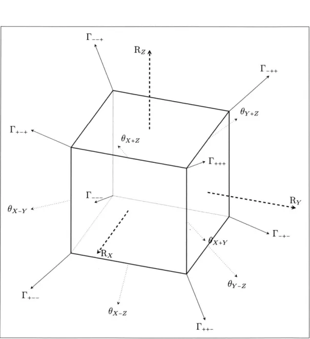
2-1 Single-qubit gates as symmetries of the cube . . . . 29

2-2 CNOT expressed as a

C(Z,

2-3

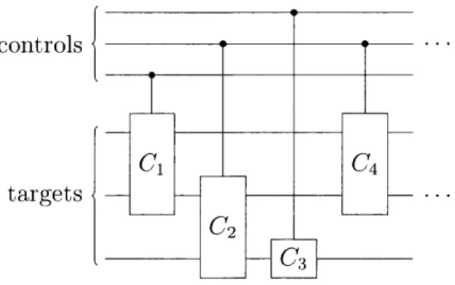
CCC circuit for Clifford gatesC

,

,

H, S}. . . . .

33

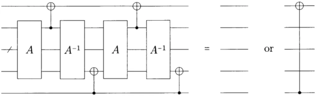
2-4 Construction of CNOT if top right entry of A is equal to 1. . . . . 38

3-1 A full description of p, the local update rule. . . . . 48

3-2 The update rule p' (suppressing symmetries) on white and gray blocks. 51 3-3 Basic operations for manipulating a signal. . . . . 54

3-4 An example of a small computation on bits X1, x2, X3. . . . . 58

4-1 Circuit diagram for CNOT(b, 1, 2) gate. . . . . 74

4-2 The inclusion lattice of degenerate Clifford gate classes . . . . 79

4-3 Inclusion lattice of non-degenerate Clifford gate classes. . . . . 80

4-4 Generating Rz with

and C(Z, Z). . . . .

93

4-5 Generating C(Z, Z) with T4 and Rz. . . . -. -. . . 94

4-6 Universal Construction €(G) . . . . 95

4-7 Decomposition of €(G). . . . . 97

4-8 Intermediate circuit in gate extraction. . . . . 98

4-9 Generating CNOT from Fredkin and NOT gates . . . . 106

4-10 The inclusion lattice of classical gates using quantum ancillas . . . . . 107

4-11 Canonical form of a 2-qubit circuit: optional SWAP gate, optional

C(P,

Q)

5-1 Quantum circuit for the Parity Halving Problem on 3 bits, PHP3

.

5-2 Grid Implementation of a Poor Man's Cat State . . . . 133

6-1 Example of a single-qubit Clifford gate gadget . . . . 164

6-2 CCCO circuit for two round protocol for gates C1,..., Ck in the first round, and gates D1,..., Df in the second round. . . . . 170

6-3 S6 = C2

/P2

6-4 The magic square game . . . . 177

6-5 Conjugating CZ and R2 by CNOT. . . . . 188

6-6 M agic pentagram . . . . . 189

6-7 Even-Odd sorting network: given any permutation, there is some sub-set of the SWAP gates above that implements that permutation. . . . 192

List of Tables

2.1 Single-qubit gates . . . . 30 2.2 Two Q ubit G ates . . . . 32

4.1 Invertible tableau elements and the corresponding single-qubit gates produced by the universal construction. Row of the table corresponds to the sign bit of the row of the tableau in which the element occurs. 74 4.2 Noninvertible tableau elements and generalized CNOT gates . . . . 74 4.3 Rules for coalescing generalized CNOT gates, assuming FPft =

Q

F Q F t= R . . . . 109 6.1 Generators for the ZX-calculus. For each green generator listed above

for the Z-basis, there is an analogous red generator for the X-basis. By convention, a solid green/red circle implies that a equals 0. . . . . 162 6.2 Rules for the ZX-calculus. In every rule, red and green nodes can be

exchanged .. . . . . 162 6.3 Operationsf EH3 which distinguish Did, from

Dc

,.

Chapter 1

Introduction

In recent years, we have seen an unprecedented new wave of investment in quantum hardware. Established tech giants, ambitious start-ups, and university labs around the world have finally begun the race for quantum computers in earnest. Over the last six years1, for example, Google has moved from cautiously benchmarking of D-Wave devices, to constructing their own 72-qubit [68] quantum architecture. These devices (and others like them) appear to be the precursors of general-purpose quantum computers, if they can overcome the high error rates and limited number of qubits they have at present. We assume that with time, researchers will find a way to lower the error rate below the critical threshold for quantum computer and then, as with conventional computers decades ago, scale up the size of the devices (i.e., number of qubits) to the point where full-scale quantum computation is possible.

An important milestone for these quantum hardware groups is the first demon-stration of quantum advantage or quantum supremacy, i.e., some computational task for which quantum devices outperform classical devices. A quantum advantage is crucial to convince skeptics (and more importantly, investors) that quantum devices are not snake oil, and that some fundamentally different, new form of computation is evident. Any particular demonstration will have detractors, so we expect there will be a sequence of increasingly convincing quantum advantage experiments until only the most die-hard detractors of quantum computing are left unpersuaded. Indeed, we may have already seen the first example: although the verdict seems to be that D-Wave's devices did not live up to their marketing (or indeed, surpass the classical state of the art), there was enough doubt about how their quantum annealing algo-rithms compared to the best classical algoalgo-rithms that it spurred further investigation by Google [40], and the computer science community in general

[79,

The push for a quantum advantage is not just the purview of hardware engineers; there has been significant progress on the theoretical side too. From the beginning, interest in quantum computing has been motivated by the idea that quantum comput-ers could be more powerful than classical computcomput-ers. That is, the class of problems solved by quantum computers in polynomial time, BQP, is separate from the class of problems that can be solved by classical computers with randomness in polynomial

time,

BPP.

Proving such a separation unconditionally is beyond current techniques

in complexity theory,

_{but there are some convincing conditional results on the}

the-oretical side.

Initially, it was assumed there would be a quantum advantage for the task of

simulating quantum systems

[48].4

physical quantum systems can be simulated efficiently, even classically, but some cases

appear to require exponential time. A universal quantum computer could plausibly

simulate the same systems in polynomial time (for a substantial quantum advantage).

However, this is bordering on tautological, like saying that simulating an NP machine

is an NP-complete problem. The first concrete evidence of a quantum advantage

came from Deutsch-Jozsa

[41],

separating EQP and P in a black-box query model

of computation, and Simon's algorithm

[107]

improved this to a separation of BQP

and BPP (again, only in the query model). Shor's algorithm

[105]

solves another

problem, factoring, which is thought to be hard classically (at the very least, we

do not have even a quasipoly-time algorithm yet), but unlike simulating a quantum

system, factoring is a very natural, number-theoretic problem which has been studied

for centuries.

Around 2010, Aaronson and Arkhipov [2] introduced boson sampling, showing

that there could be an advantage for a non-universal quantum device built using

lin-ear optics, and using a sampling task rather than a conventional decision problem.

Unfortunately, linear optical devices have proved difficult to scale up to the point

that the Aaronson-Arkipov proposal would be classically intractable. Independently,

Bremner, Jozsa, and Shepherd [29] gave a similar result with similar hardness

as-sumptions, but using a commuting gates model instead of linear optics. The weakest

versions of the Aaronson-Arkhipov and Bremner-Jozsa-Shepherd results require the

(quite reasonable) conjecture that the polynomial hierarchy does not collapse, and

stronger versions (usually to sample within additive error) require domain-specific

conjectures about, e.g., the permanents of matrices with random Gaussian entries,

or anti-concentration of amplitudes in IQP circuits. Sampling results also include

random circuit sampling, the problem of measuring a sample from a quantum circuit

of randomly chosen gates, with various choices of depth, topology, and gate set of

the circuit. Variations of random circuit sampling are the basis of several competing

proposals [21] for demonstrating quantum effects in near-term devices, although they

often fall somewhat short of a rigorous quantum advantage, one main exception being

2

Whether polynomial time (either P or BPP) captures the efficient computation is a big question on its own, going back to Cobham [32] or Edmonds [45] in 1965. It is even less clear that polynomial time captures efficiency for quantum computations, since the same arguments against the idea still apply (e.g., constant factors could be large, big exponents are not especially efficient) and, for now, we lack real world evidence with quantum computers to support it. We adopt the orthodox view that P, BPP, and BQP capture "efficient" or "tractable" problems, although we will have little use for these classes within this thesis.

3

1n _{particular, P c BPP and BQP c PostBQP c PSPACE, so a separation would settle the open}

question of whether P = PSPACE negatively. This would be an enormous breakthrough.

4

In a single quote: "Nature isn't classical, dammit, and if you want to make a simulation of nature, you'd better make it quantum mechanical, and by golly it's a wonderful problem, because it doesn't look so easy."

that of Bouland et al.[23].

Notice that in these quantum supremacy proposals, there is a trend over the years towards what is practically realizable on quantum devices in the near future. Early theoretical results were understandably focused on establishing that quantum com-puters are a worthwhile goal, potentially useful in some hypothetical sci-fi future. As experimental progress is made, the proposals get closer to might soon be achievable, e.g., using linear optics because the hardware looks promising (photons are in some ways easier to manage than other quantum media). The theoreticians are meeting the experimentalists in the middle, so to speak, and in this thesis we argue that is a good thing. Adapting theoretical results (and especially the models of computation) to the realities of near-term quantum devices can only hasten the advent of quantum supremacy. Moreover, some limitations of current quantum hardware may persist well into the future, so there is value in adapting our models of computation to the devices.

This thesis is a collection of results about models of computation (i.e., mathe-matical descriptions of computational devices, suitable for proving theorems about). In each case, the model captures some aspect or limitation of near-term quantum devices (NTQD), and thus contributes to our understanding of those devices. There are three properties which appear again and again, which are themes (and therefore chapters) of this thesis.

1. The topology of qubits in NTQDs tends to be a two-dimensional grid. Being able to implement quantum gates between arbitrary pairs of qubits is probably

not realistic in the near-to-intermediate future, so expect local gates.

2. The Clifford gates are a special gate set in several areas of quantum comput-ing. While we do not expect Clifford gates to be the only gates available on NTQDs, they may be easier, cheaper, or more reliable to implement. If we can make our circuit out of only Clifford gates, so much the better.

3. Depending on the implementation of qubits, coherence time puts an upper bound on the usable lifespan of any qubit. This limits the depth of any cir-cuit we can implement (at least until we have quantum error correction), so low-depth quantum circuits are the most realistic for now.

The models of computation we study are not new: quantum low-depth circuits have been studied for twenty years, cellular automata were proposed in the 1940s, and the Clifford group was of mathematical interest in the nineteenth century. Neither are the models of computation especially realistic or fine grained: in a long tradition of theoretical results, we are interested more in asymptotic behavior than constant factors, even when the constant factors are prohibitive. Our goal is merely to explore these three limitations of near-term devices in a mathematically precise way.

We devote Chapter 2 to notation and background. Experts should skim it for our notation for Clifford gates and complexity classes in particular. The meat of the thesis is in the four chapters after that on grid topology (Chapter 3), Clifford gates (Chapter 4), and two chapters on low-depth quantum circuits (Chapter 5 and Chap-ter 6). Do not be surprised to find these concepts outside their respective chapChap-ters,

since they are the themes of this thesis, not merely chapter headings. Let us briefly

discuss each of the three themes before we continue.

First, for the popular quantum architecture of superconducting qubits, quantum

information resides in superconducting islands, i.e., physical structures on a chip. The

fabrication techniques used for quantum chips are not so different from conventional

integrated circuits, and in particular they arrange the qubits on a plane. In principle

one could arrange the qubits in any planar configuration on the chip, but designers

naturally tend toward regular grids, since then any qubit in the middle of the grid has

a similar neighborhood and hopefully similar circuitry. With sufficiently many qubits,

it is no longer practical to connect every pair of qubits directly, and the architecture

shifts towards connecting only nearby qubits (again, making the connections regular

may simplify matters). Thus, we expect qubits on a plane, in a grid topology, with

local gates between neighbors-and this is exactly what we see in 50+ qubit designs

of IBM, Google, and D-Wave [68, 221.

The Clifford gates are interesting enough in their own right to deserve study.

In keeping with the theme, however, there are also reasons to believe Clifford gates

will be especially important for quantum devices in the future. Some quantum error

correcting codes have the feature that some gates can be implemented transversally on

encoded qubits, i.e., by applying the gate to each physical qubit in all logical qubits.

That is, in a code with k physical qubits per logical qubit, transversal operations are

performed with k gates. Unfortunately, at most the Clifford gates can be transversal,

and they are insufficient for universal quantum computation. There are proposals to

achieve universal computation with encoded qubits, but in at least one notable case

(using magic states, or IT) states) the non-Clifford gates dominate the cost to the

extent that Clifford gates are counted as "free". At any rate, under any quantum code

with the transversal property, we can expect the Clifford gates to be the cheapest to

implement.

Last, we consider low-depth circuits. Qubits have limited lifetimes, in the sense

that the time until an error occurs follows an approximately exponential distribution.

On real, current devices with superconducting qubits, the mean time to error is in

the tens of microseconds

[731.

Even at a clock rate of a few gigahertz (comparable

to modern classical devices) the quantum device can perform fewer than 105 gates

on a particular qubit before it should expect an error. Lowering the error is a major

engineering challenge, and mitigating the error with quantum error correcting codes

is not yet feasible either, and even once it is possible, error correction will require

additional qubits and gates to implement. For now, the best way to minimize this

kind of error on a qubit is to minimize the length of time the qubit needs to exist

coherently. The time required to execute a circuit can be approximated by its depth

(up to constant factors, perhaps), so we wish to study low-depth quantum circuits.

Furthermore, low-depth classical circuits have enjoyed over four decades of fruitful

study, so it is natural to study analogous quantum device (as evidenced by two decades

of low-depth quantum circuit study).

Each chapter presents a different result, so let us briefly summarize them before

5

continuing. Theoretically, grid based computation does not present much difficulty, so Chapter 3 considers an extremely constrained grid-based model of computation, the cellular automaton. We show that a particular cellular automata satisfies a very stringent universality property, and take this as evidence that computation in a grid is possible even under extreme circumstances. Next, Chapter 4 classifies the power of arbitrary subsets of Clifford gates. It turns out a collection of Clifford gates generates one of 57 different subsets of Clifford operations, and we enumerate all of these classes to better understand the structure within the Clifford group from the perspective of building quantum circuits. This brings us to our two low-depth quantum circuit results, which both build off of a recent unconditional separation of shallow circuit classes: constant-depth quantum circuits can do something constant-depth classical circuits cannot

[26].

Chapter 2

Background

In this chapter, we briefly introduce the basic concepts and notation for quantum computing with qubits. We also discuss universality, the Pauli group and Clifford group, common gates, and relevant complexity theory.

2.1

Qubits, Measurement, and Quantum Gates

Mathematically, a qubit is the set of unit vectors (under the f2 norm) in a

two-dimensional Hilbert space. The two classical basis or Z basis vectors are called

|0)

|0) :=

,0l

(11)1

_:

(0).

The symbol 1.) is a "ket", and it denotes a complex vector labeled by the contents of the ket. As you can see, 10) and 11) are just the standard basis vectors eo and ei. We also define the X basis vectors,

0)+1)

1

10)

-1 1)

(1

On the other hand, when we write, e.g.,

|x

{0,

|0)

|1)

For this thesis, most of the models of computation are built on a finite array of qubits. Since a bit has two states and a qubit is a two-dimensional Hilbert space, by analogy we use a 2m-dimensional Hilbert space to represent an array of m qubits. Canonically, we construct this space by taking the tensor product, denoted ®, of m two-dimensional Hilbert spaces (i.e., qubits). The states for an m-qubit system are the unit norm vectors in this 2m-dimensional Hilbert space.

We can also take the tensor product of vectors, e.g., the m-fold tensor product of

10),

is a state on m qubits. The tensor product symbol is omitted in practice as much

as possible, so this would typically be written 10)|0) --- 0). We define the m-qubit

classical basis vectors 0...0),0--1),... ,1 ... 1) as

|bl---.bm) :=|Jbi) (9 --- 9 1|bm)

where bi,...,

{0,

1} are bits. Thus, all of the following states are equivalent:

|0)"m = 10) & --- (& |0) = |0) --- |10)

|0---.0)

|0m).

Measurement (in the Z-basis) of a single-qubit state

1)

a0) + |1)

collapses it to either 10) with probability

or 11) with probability

and in the

process we learn which outcome has occurred. The probabilities sum to one because

#)

la|2

)=

)

returns Ix) with probability

lar|2,

and again the probabilities sum

to one because 10) is a unit vector. More generally, orthogonal measurements divide

the Hilbert space into orthogonal subspaces and project the state onto a subspace

with probability proportional to the square of its component in that subspace. For

example, measuring just the first qubit of 10) gives the state

XE,ln-1olf with probabilityZ{o,in-iaO2

ZExEO,lnl _|E~ 21xlX

with probability

~n-1

jXE{Oi1)n-ic01iaJ

X

In this thesis, we are interested in models of quantum computation built on qubits.

That is, we start with the qubits in some initial state, manipulate them by some

sequence of quantum operations, then measure. Furthermore, we will consider only

models of computation where the quantum operations applied in discrete steps (i.e., a

gate model), though it is worth mentioning that continuous time models exist where

quantum operations can, e.g., continuously rotate 10) to 11) through I+). A quantum

gate is linear map U from the Hilbert space (however many qubits) to itself, mapping

quantum states to quantum states, i.e., preserving£2 norm. One can show that the

f2

norm is preserved if and only if U is a unitary matrix, i.e.,

UUt

UfU = I,

where Ut is the Hermitian conjugate of U. Clearly the inverse of U is Ut, and the

product of two unitaries is unitary, since

UV(UV)t

UVViUt = UIUt = UUt = I.

group, denoted U(d).1

In both classical and quantum circuit models, we do not assume we can implement

arbitrary gates (i.e., arbitrary Boolean functions classically, or arbitrary unitaries

quantumly). For one, an arbitrary gate has an exponentially long description (as-suming an approximate unitary quantumly). Instead, one typically assumes a small set of gates with constantly many inputs, and perhaps a uniform family of gates on an unbounded number of inputs. Classically, one takes the AND, OR, and NOT gates, or simply the NAND gate, or all 1- and 2-bit gates. These can be augmented by unbounded fan-in gates for AND and OR, or for PARITY, MOD functions, MA-JORITY, and so on. Quantumly, the situation is similiar: we take some subset of 1-and 2-qubit gates which is universal in the sense that the gate set can simulate all quantum gates. For example, the CNOT gate defined below, and the set of all (n.b., uncountably many) single qubit gates is universal.

Fact 1. The CNOT gate and the set of all single-qubit gates are universal for quantum

computing in the sense that any unitaryUEU(2m) on m qubits may be implemented exactly with a circuit of these gates.

2.1.1

Quantum Gates

We know in the abstract that quantum gates are unitaries, acting on a small number of qubits. Let us see some examples used in practice, starting with the reversible gates, which permute the classical basis states.2 These correspond to permutation matrices on 2m dimensions, and every permutation matrix is unitary so they are immediately quantum gates as well, acting on quantum states by linearity.

First among the reversible gates is NOT, which flips the input, exchanging 0 and 1, the only non-trivial 1-bit reversible gate. Next, the SWAP gate is a 2-bit gate which exchanges the two bits, i.e., exchanges 01 and 10. The controlled-NOT or CNOT gate is a 2-bit such that input

(x,

(x,

e

x, y E

{0,

and the gate is like applying a NOT gate to target if and only if the control bit is 1. In the same vein, the controlled-SWAP gate (or CSWAP or Fredkin gate) swaps the second and third (target) bits if and only if the first bit is 1. And finally, we have the controlled-controlled-NOT gate (or CCNOT or Toffoli gate), where a (singly)

'There is also a question of phase. If we recall the definition of quantum measurement, notice that nothing changes if we multiply the entire state by eio, in that the measurement outcomes occur with the same probabilities, and the states afterward are multiplied by eO. For this reason, people say the global phase of a quantum state is irrelevant. It follows that we wish to treat all unitaries of the form e'0I as equivalent, so we are actually interested in the projective unitary group, PU(d), defined as the quotient of U(d) by its center, the set of unitaries of the form ei0I.

2

As background, reversible computing was proposed (before quantum computing) as a remedy to Landauer's principle, the idea that destructive operations (e.g., erasing a bit) must consume energy as a consequence of thermodynamics. To avoid this cost, the computation needs to be reversible physically, and therefore also reversible logically, and remarkable work of Bennett [15] shows this is possible. Reversible gates are logically reversible and therefore useful in reversible computation, hence the name.

controlled-NOT gate is applied to the second and third bit if the first bit is 1, i.e.,

(X, y,

- (X, y, zy

z).

In addition, we define some common quantum gates. The controlled-sign gate (or

CSIGN or CZ) flips the global sign if and only if both inputs are 1, i.e., the diagonal

transformation

(1 0 0

0)

CSIGN

0 0 0 -1/

Similarly, the phase gate, traditionally either S or P (we opt for S), is diagonal:

S:=

(a?).

Last but not least, the Hadamard gate is H =

(

1 _

).

2.2

Pauli Group and Clifford Group

An entire chapter of this thesis (Chapter 4) is devoted to the Clifford gates on qubits,

and they are ubiquitous in quantum computing. We have already seen many Clifford

gates above, but let us formally define the Clifford group, and before that, the closely

related Pauli group.

2.2.1

Pauli Group

First, recall the Pauli matrices, a collection of four 2

2 unitary matrices:

1

0 i 1

0

0 1 '1 0 'i 0 '0 -1

Since the Pauli matrices satisfy the relations

X-Y=iZ,

Y-X

= -iZ,

Z.Y= -iX,

_{X- Z = -iY,}

X2 =2 = Z2 I

and I is an identity element, the set P1

:=

{±1,±i}

{I, X, Y, Z} is a group under

multiplication. This is the one-qubit Pauli group, and it generalizes to the m-qubit

Pauli group Pm :=

{

±1,

{I,

tensor product of the Pauli matrices, which we call a Pauli string, and a

{±1,±i}

component which we call the phase. We typically omit the tensor products in the

Pauli string when possible, e.g., writing IXYZ for I X 9 Y 9 Z.

Let us name the group of phases

{±1,

I", and note that

is a normal

subgroup of

This means the quotient

Pm/Zm

is well-defined. Each element of

Pm/Zm

is a coset

{+P,

-P,+iP, -iP} for some P

E

{I,

X, Y, Z}©m, but we identify each

such element with P, its positive representative.

Fact 2. Any matrix AE C2mx2" can be written as a complex linear combination of

{I,

Define the notation G(b1,..,in) := G1 -- Gm where G is a unitary gate and

(bi,..., bn) E Z is an integer vector. Another useful fact is that there are subsets of 2n Pauli elements which generate the whole group up to phase.

Fact 3. Any P e Pm can be written in the form P := aXa awhere a c

{

a,b E IF". Since 1,..., - generates (by multiplication in the group) all Xa and

e1,... ,

Z-generates

Finally, although the Pauli group is not abelian, it has the property that any two elements either commute or anti-commute.

Fact 4. For all P,Q E Pm, the commutator [P,

Q]

2.2.2

Clifford Group

Define the m-qubit Clifford group, Cm, as the set of m-qubit unitaries (under multi-plication) normalizing the m-qubit Pauli group,

Cm := {U E U(2") : UPmUt = Pm}.

That is, a unitary U E U(2m) is Clifford if for any P E Pm, conjugation by U gives

an element of Pm. It is immediate that this is a group, and by construction Pm is a normal subgroup of Cm, i.e.,

Zm ! Pm Cm.

Since conjugation of a Pauli by a Clifford operation is so common, we define the notation . : Cm xPm - Pm where U * P:= UPUt for any U E Cm and P E Pm.

This definition is a quite abstract, so let us give some examples. First, perhaps obviously, the SWAP gate is a Clifford gate since

SWAP(XI)SWAPt = IX, SWAP(IX)SWAPt = XI,

SWAP(ZI)SWAPt

IZ,

SWAP(IZ)SWAPt

ZI.

It suffices to check that XI, IX, ZI, IZ are mapped to Pauli strings because of Fact 3. Any other Pauli string can be written as a product of these elements, and since

U(PQ)Ut = (UPUt)(UQUt), will be transformed to a product of Pauli strings.

Similarly, CNOT is a Clifford gate:

CNOT(XI)CNOTt _{= XI, CNOT(IX)CNOTi =}

IX,

CNOT(ZI)CNOTt = ZI,

CNOT(IZ)CNOTt

IZ.

±P for all P,

Q

E Pm. The Hadamard gate (H) and phase gate (Rz) are also Clifford:

HXHt = Z, SXSt = Y,

HZHt =

X,

The surprising fact, however, is that CNOT, Hadamard, and Phase generate the

entire Clifford group.

Theorem 5. Every element of U E Cm can be constructed

from a

H, and Rz gates.

We define a Clifford circuit as any quantum circuit built from a basis of Clifford

gates, with

{CNOT,

H, Rz} being one possible basis (for the entire group, by

Theo-rem 5). A Clifford state or stabilizer state is any quantum state of the form U 0)0m,

whereUE U(2m) is Clifford. A equivalent way to define a Clifford state is by its

stabilizer group,

Stabp

E

Pm : P I)) = |V)},

the set of Pauli elements which fix the state. The X-basis

(1+),

1-)), Y-basis

(Ii),

-i)), and Z-basis

(10),

11)) states are all trivially stabilizer states, where

10)

i l1)

10) - i

ll)

The cat state

is also an example of a Clifford state.

The Clifford gates are not universal for quantum computing, which is hardly

surprising given that Cm is a discrete, finite group for any particular m. In fact, the

Clifford gates are classically simulable, not only in P, but in the complexity class (L

[4].

We discuss complexity classes in Section 2.3.

2.2.3

Clifford Tableaux

An important representation for Clifford operations (and a good way to prove a

simulation result) is the tableaux representation. In this section, we explain how

tableaux can be derived from first principles, going as far as we need for general

background and Chapter 6. The Clifford chapter, Chapter 4, will require a more

extensive treatment (see Section 4.2).

Observe that any unitary can be defined (up to phase) by how it conjugates

density matrices, i.e., by the set

{(p,

UpUt) : p > 0}. Since the Pauli group forms a

basis for all matrices, this can be reduced to the set

{(P,

UPUt) : P E Pm}. In fact,

since Xe

, Xem,

generate

and conjugation preserves produces (i.e.,

UPUtUQUt

=

it suffices to write down UXiUt and

for all i. When

U is a Clifford unitary, we also get that UXeUt and

are in Pm. For example,

SXSt = Y and SZSt = Z, from which we can derive that

Clearly SISt = I, and thus we can derive SpSt for any p by linearity. Similarly,

HXHt = Z, HZHt = X and

CNOT(XI)CNOTt = XX, CNOT(IX)CNOTt = IX,

CNOT(ZI)CNOTt = ZI,

CNOT(IZ)CNOTt = ZZ.

In general, a Pauli operator P = aXaZb E Pm can be represented with two n-bit vectors a,bE IF' and a pair of bits for o, and any Clifford operation is defined by 2m

Pauli operators UXeUt,..., UXUt, UZe1Ut,..., UZemUt, the entire operation can be described by a matrix of 2n rows with 2m+2 bits per row. The phase information can be reduced to one bit per row (instead of two) to give a tableau, but since we will not need that part of the tableau for most of thesis (only in Chapter 4, and we have a separate discussion of Clifford tableau), we will skip it and focus on the remaining 2m x 2m binary matrix.3 We divide the matrix into four blocks,

I A BI

where A, B, C, D E FTn. That is, the ith row of A records the X component of the Pauli string UXeiUt, and the ith row of B represents the Z component of the same Pauli string. Similarly, the ith row of C and D represent the X and Z components of the Pauli string UZeiUt. Then we have the following facts.

Fact 6. The tableau [ ] corresponds to a Clifford operation if and only if it is

symplectic. The matrix is symplectic if and only if ADT + BCT = I and both ABT

and CDT are symmetric.

Fact 7. Let U c C, be a Clifford unitary with tableau

[

(r s) C D) =u (UV).

₍

A B

It follows that, ignoring phase, the tableau for a unitary VU is the standard matrix product of the tableau for U and the tableau for V.

We have not seen complexity classes yet, but matrix multiplication over IF2 is in

@L. Hence, we can simulate a sequence of Clifford gates in

eL.

[4],

2.2.4

Clifford Gates

In our final background subsection on Clifford gates, we make a thorough study of single-qubit Clifford gates (which happen to correspond to symmetries of cube, see

3

One can check that for all X and Zb, the phase of UX"Ut and UZbUt is either +1 or -1 for all

Figure 2-1), and then the named multi-qubit Clifford gates.

2.2.5

Single-qubit Gates

We group the gates by the type of rotation to emphasize this geometric intuition.

Face rotations: The Pauli matrices X, Y, and Z (as gates) correspond to 180°

rota-tions about the X, Y, and Z axes respectively. Similarly, we define Rx, Ry, and

Rz to be

900

rotations (in the counterclockwise direction) about their respective

axes. Formally,

XI-iX

Rx

Rz

although in the case of Rz (also known as the phase

gate

and often denoted

by S or P), a different choice of phase is more conventional. The clockwise

rotations are then Rt, Ry and R.

Edge rotations: Another symmetry of the cube is to rotate one of the edges 180°.

Opposing edges produce the same rotation, so we have six gates: Ox+y,

0

_{x+z, x-z}

_{y+z, Oy-z. We define}

P+Q

P-Q

.Q =

,'2

_{BeQ =}

_2,

for all Pauli matrices P

Q.

Note that Ox+z is the well-known Hadamard gate,

usually denoted by H.

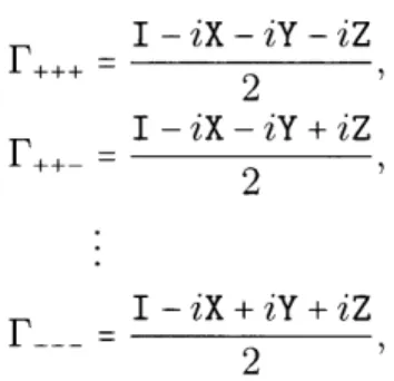
Vertex rotations: The final symmetry is a 120° counterclockwise rotation around

one of the diagonals passing through opposite vertices of the cube. The cube

has eight vertices, (+1, +1, ±1), and we denote the corresponding single-qubit

gates F ..

,

I -iX - iY - iZ

2

I-iX

2

iX+iY+iZ

2

We also define F (without subscripts) to be the first gate, F+++, since it is the

most convenient; conjugation by F maps X to Y, Y to Z, and Z to X.

RzA

IF-+

OY-Z

Ox-z

F++

Figure 2-1: Single-qubit gates as symmetries of the cube

Fx+z

x+y

Unitary Matrix

x

Y

Z

Oxz =

x+z =

H

0x-z

F+++

Table 2.1: Single-qubit gates

2.2.6

Multi-qubit Gates

We now introduce some multi-qubit Clifford gates. We have already seen the SWAP

gate and the CNOT gate. A generalized CNOT gate is a two-qubit Clifford gate of

the form

I®I+P®I+I®Q-P®Q

C(P, Q):=

2

2

where P and

Q are Pauli matrices. If the first qubit is in the +1 eigenspace of P then

C(P,

Q)

does nothing, but if it is in the -1 eigenspace of P then C(P,

Q)

applies

Q

to

the second qubit. Of course, the definition is completely symmetric, so you can also

view it as applying P to the first qubit when the second qubit is in the -1 eigenspace

of

Q.

Observe that C(Z, X) is actually the CNOT gate; Figure 2-2 shows this equivalence,

and illustrates our circuit diagram notation for generalized CNOT gates. Also note

that C(X, Z) is a CNOT in the opposite orientation. The rest of the heterogeneous

generalized CNOT gates (i.e., C(P,

Q)

where P #

Q)

are the natural equivalents of

CNOT in different bases.

Similarly, C(Z, Z) is better known as the controlled-sign gate (denoted CSIGN or

CZ), which flips the sign on input 111), but does nothing otherwise. The homogeneous

generalized CNOT gates (i.e., C(P, P) for some P) are quite different from

hetero-geneous CNOT gates. For instance, when one CNOT targets the control qubit of

30

0

0

0 0

10

110

0 0

1 1

0 1

1 0

0 0

)

-i

1)

-1

1

-1

-1

1

1

-1

i

)

)

)

)

)

)

Z

X

Figure 2-2: CNOT expressed as a C(Z, X) gate

another CNOT then it matters which gate is applied first. On the other hand, two CSIGN gates will always commute, whether or not they have a qubit in common.

It turns out that every two-qubit Clifford gate is equivalent (up to a SWAP) to some combination of one qubit Clifford gates and at most one generalized CNOT gate (see Section 4.9.4). Most classes of Clifford gates are of this form, but there are a handful of classes which require larger generators such as the T4 gate [5, 53]. For all

k > 1, we define T2k as the 2k-bit classical gate that flips all bits of the input when the parity of the input is odd and does nothing when the parity of the input is even. In particular, T2 is the lowly SWAP gate. Notice that T2k is an orthogonal linear function of the input bits. The matrix of the T4 gate (over F2) is

0 1 1 1) 1 0 1 1

1 1 0 1

1

I

1 0

In the quantum setting, define the T2kgate as apply this linear transformation to the Z basis vectors.

2.3

Computational Complexity

We assume a familiarity with Turing machines and the basic complexity classes:

• P: decision problems solvable in polynomial time, " L: decision problems solvable in logarithmic space,

" NP and NL: decision problems solved by non-deterministic versions of the above, " PSPACE: decision problems solvable in polynomial space.

We will also need DL, the class of decision problems solved by an NL machine where we accept if the machine has an odd number of accepting paths and reject if the machine has an even number of accepting paths (i.e., perfectly analogous to &P, but logarithmic space).

Now let us define some standard polynomial-size circuit families. For each of the families below, we adopt the convention that Ci denotes the subfamily of circuits in

GateTabeau

Uniaryatrioncmpuatinalasi

C(XjX)

C(YY)

C(Z, Z)

CSIGN

C(Yj X)

C(ZY)

C(X, Z)

CNOT

1 0 0 1

10 1 0

0

0 1 1 0

0 0

10

1

11 0 1

0

010 1 10

00

1 0 0

1 1

10

1

0 1 0 1

1 0 0 0

0 0 0 1

(1

11

1

1

-1

(ii

1-1 -1

1

-1

1

1 1

1

1

-1

i i 1/

0 0

0

0 0

1

1

i

--i 11

0 0

0

1 0

0

0 i0

0 0 0\

1 0 0/

Table 2.2: Two qubit gates. The sign bits are all 0 in the above tableaux so they are

omitted. In this table, we adopt the convention (from Chapter 4) that the Pauli basis

elements are XI, ZI, IX, IZ in that order.

Unitary Matrix on computational basis

"

NC:

classical circuits of bounded fan-in AND, OR, and NOT gates.

"

AC:

classical circuits of unbounded fan-in AND, OR, and NOT gates.

•

QNC:

quantum circuits of CNOT gates and arbitrary single-qubit gates.

"

Clifford: quantum

circuits of CNOT, Hadamard, and -Phase gates.

Let us now define another

quantum

circuit family, CCC, the classically-controlled

Clifford circuits.

Definition 8. A classically-controlled Clifford circuit is a quantum circuit of Clifford

gates where some gates are labeled by a individual bits of the classical input. To

execute a classically-controlled Clifford circuit on an input, we remove Clifford gates

labeled by a 0 input bit and keep the unlabeled gates or those labeled by a 1 bit.

Then run the quantum circuit as usual.

The name comes from the concept of a controlled gate. Given any n-qubit gate

G, we can define an (n

controlled gate

XG:=(I + X) (& In + (I - X) (& G

X(G) :=

2

which applies G to the last n qubits (the target qubits) if and only if the first qubit

(the control qubit) is 1. For example, CNOT is literally a controlled NOT gate, X(X).

An alternative definition of CCC is a quantum circuit with the input partitioned

into control bits and target bits, where controlled Clifford gates (e.g., CCNOT,

C-Hadamard, C-Phase, CZ) are allowed from the control bits to the target bits and

arbitrary Clifford gates are allowed on the target bits. The classical input appears as

the initial setting of the control bits. See Figure 2-3 for an example circuit.

controls

C1 C4

targets

C2

- C

Figure 2-3: CCC circuit for Clifford gatesC

C

,...

{CNOT, H, S}.

We also note two important subclasses of the classically controlled Clifford gates.

o L/poly: the family of classically controlled Clifford circuits where the only gates

*eL/poly: the

family of classically controlled Clifford circuits where the only

gates are controlled or not controlled versions of CNOT and X (i.e., NOT).

The names of the classes (deliberately) suggest that they are related to the Turing

machine classes L and EL. The notation /poly means they are given polynomial-length

classical advice. In other words, the class is augmented with an (by default, classical)

advice string of polynomial length (indicated by the poly) which depends on the input

length, but not the input. This string is passed to the computational device with the

input. For example, P/poly is equivalent to polynomial-size circuits since, in one

direction the advice could encode a circuit to simulate (circuits c P/poly), and in

the other direction, any P computation can be written out as a circuit and then the

advice could be hard-coded (P/poly c circuits).

As the names suggest, these two classically controlled Clifford circuit classes indeed

align with advice classes.

Theorem 9. The class of decision problems solved by a family of L/poly classically

controlled Clifford circuits is the advice class L/poly. Similarly, the class of decision

problems solved by a family of e L/poly classically controlled Clifford circuits is the

advice class e L/poly. Note that the solution to a decision problem is encoded (for this

kind of computational device) by the value of the top bit at the end of the computation.

Proof. A result of Cobham

[33]

says that L/poly (the advice class) is equivalent to

polynomial-length, polynomial-width branching programs. For the unfamiliar, a

de-terministic branching program is a computational device consisting of a layered

di-rected graph, where the edges of the graph are labeled by input bits and there is only

one outgoing edge for each label. A result of

[74]

says that log space is equivalent

to reversible log space, which improves the Cobham result by asserting the layers of

the branching program are permutations. We leave it as an exercise to verify that a

polynomial-length, polynomial-width branching program of permutations is

equiva-lent to a network of swaps

(i.e.,

the classically controlled Clifford circuit class) and

thus to L/poly.

Computing the product of a network of CNOT gates is complete for EL according

to a survey of Damm

[39].

It follows that a

oL/poly

family of classically controlled

Clifford circuits can be simulated in e L/poly, where the advice is to specify the circuit.

Conversely, given a eL machine that uses advice, translate it to a network of CNOT

gates and then hardcode the ones that depend on the advice.

D

It will be handy to have circuit characterizations of these Turing machine classes,

since we are about to define several kinds of computational problems from circuit

families.

Traditionally, a complexity class is a set of computational problems, often the set

of problems solved by a particular device under certain resource constraints (e.g.,

limited time/space or depth/size) and acceptance conditions (e.g., the device counts

as answering "yes" if it says yes on at least i of random inputs). There are many

kinds of computational problems: