HAL Id: hal-00341613
https://hal.archives-ouvertes.fr/hal-00341613
Submitted on 25 Nov 2008HAL is a multi-disciplinary open access
archive for the deposit and dissemination of sci-entific research documents, whether they are pub-lished or not. The documents may come from teaching and research institutions in France or
L’archive ouverte pluridisciplinaire HAL, est destinée au dépôt et à la diffusion de documents scientifiques de niveau recherche, publiés ou non, émanant des établissements d’enseignement et de recherche français ou étrangers, des laboratoires
Setting port numbers for fast graph exploration
David Ilcinkas
To cite this version:
David Ilcinkas. Setting port numbers for fast graph exploration. Theoretical Computer Science, Elsevier, 2008, 401 (1-3), pp.236-242. �10.1016/j.tcs.2008.03.035�. �hal-00341613�
Setting Port Numbers for Fast Graph Exploration
David Ilcinkas∗CNRS, LaBRI, Universit´e Bordeaux I, France [email protected]
Abstract
We consider the problem of periodic graph exploration by a finite automaton in which an automaton with a constant number of states has to explore all unknown anonymous graphs of arbitrary size and arbitrary maximum degree. In anonymous graphs, nodes are not labeled but edges are labeled in a local manner (called local orientation) so that the automaton is able to distinguish them. Precisely, the edges incident to a node v are given port numbers from 1 to dv, where dv is the degree of v.
Periodic graph exploration means visiting every node infinitely often. We are interested in the length of the period, i.e., the maximum number of edge traversals between two consecutive visits of any node by the automaton in the same state and entering the node by the same port. This problem is unsolvable if local orientations are set arbitrarily. Given this impossibility result, we address the following problem: what is the mimimum function π(n) such that there exist an algorithm for setting the local orientation, and a finite automaton using it, such that the automaton explores all graphs of size n within the period π(n)?
The best result so far is the upper bound π(n) ≤ 10n, by Dobrev et al. [SIROCCO 2005], using an automaton with no memory (i.e. only one state). In this paper we prove a better upper bound π(n) ≤ 4n. Our automaton uses three states but performs periodic exploration independently of its starting position and initial state.
1
Introduction
The task of visiting all nodes is fundamental when searching for data in a network. The specific case of periodic exploration is particularly useful for network maintenance, where every node has to be regularly checked. In this paper we consider the task of periodic exploration, in which a mobile entity, or robot, has to periodically visit every node of an unknown graph.
We assume that the graph is anonymous, i.e., the nodes are unlabeled. Note that node labels would not help much the robot anyway because, as we will see later, it is modeled as a finite automaton, and thus is unable to store even a single node label. To enable the robot to distinguish the different edges incident to a node, edges at a node v are assigned port numbers in {1, . . . , dv} in a one-to-one manner, where dv is the degree of node v. Such port-numbering is called a local orientation.
The robot is modeled by a deterministic finite automaton. More precisely, we consider Mealy automata. A Mealy automaton has a transition function f and a finite number of states. If the ∗Supported by the project “PairAPair” of the ACI Masses de Donn´ees, the project “Fragile” of the ACI S´ecurit´e et Informatique, and the project “Grand Large” of INRIA.
automaton enters a node of degree d through port i, in state s, then it switches to state s′ and exits the node through port i′, with f (s, i, d) = (s′, i′). Since the transition function takes as input a port number, we say that the automaton is on an edge e towards the extremity v of e or, in short, is on (e, v). Such a pair is called a position.
We consider the problem of periodic graph exploration where the finite automaton has to explore any unknown anonymous connected graph of arbitrary size and arbitrary maximum degree. Periodically exploring a graph means visiting every node infinitely often. We are interested in the length of the period, i.e., the maximum number of edge traversals between two consecutive visits of any node by the automaton in the same configuration (i.e., same position and same state). Budach [5] proved that no finite automaton can explore all graphs if the local orientation is given by an adversary. Given this impossibility result, we address the following problem:
Problem. What is the mimimum function π(n) such that there exist an algorithm for setting the local orientation, and a finite automaton using it, such that the automaton explores all graphs of size n within the period at most π(n)?
Dobrev et al. [11] presented a port-numbering algorithm, and an automaton using it, achieving a period of at most 10n for graphs of size n. Hence π(n) ≤ 10n. The main advantage of their approach is that their automaton is ultimately simple: it is oblivious (i.e. it uses only one state). Indeed their automaton uses the so-called right-hand-on-the-wall walk defined by f (s, i, d) = (s, (i mod d) + 1). Using an oblivious automaton naturally solves the problem of setting the initial state. However, the good performance of the automaton in [11] relies on the fact that the agent must start the exploration by the edge with port number 1.
In this paper we prove that π(n) ≤ 4n − 2. Our automaton is not oblivious but has only three states. Moreover, it performs periodic exploration independently from its starting position and initial state. Our port-numbering algorithm is based on a spanning tree of the graph and can be easily implemented in a distributed environment, and extended to dynamic networks.
1.1 Related work
Exploration of unknown environments have been extensively studied in the literature (cf. [20, 22]). The environment can be modeled using geometry as a plan with obstacles or as a graph. In the latter case, moves are restricted to the edges of the graph. The graph setting can be further specified in two different ways. In [4, 9, 14, 18] the robot explores strongly connected directed graphs and it can move only in the head-to-tail direction of an edge, not vice-versa. In [5, 10, 12, 13, 16, 21, 24] the explored graph is undirected and the robot can traverse edges in both directions. Again two different assumptions are used in the literature: it is either assumed that nodes of the graph have unique labels which the robot can recognize (as in, e.g., [9, 13, 21]), or it is assumed that nodes are anonymous (as in, e.g., [4, 5, 12, 24]). We are concerned with the latter context.
It is often assumed that the robot has an unlimited amount of memory to perform his task. In this paper, we are interested in robots using very little memory. More precisely we want the robots to have only a constant number of memory bits. A very natural model in this case is the finite automaton. Budach [5] proved that no finite automaton can explore all graphs. Rollik [24] proved that even a finite team of finite automata cannot explore all planar cubic graphs. This result is improved in [7], in which the authors introduced an even more powerful machine, called the JAG, for Jumping Automaton for Graphs. A JAG is a finite team of finite automata that can permanently cooperate and that can use “teleportation” to move from their current location to the
location of any other automaton. Cook and Rackoff [7] proved that no JAG can explore all graphs. It was proved later in [19] that an automaton requires at least n states to explore all graphs of size n. Reingold [23] proved a very challenging result stating that SL = L by providing a log-space algorithm solving the USTCON problem. A consequence of his work is the existence of a robot with O(log n) bits performing exploration in n-node graphs, matching the lower bound of Ω(log n) bits in [19].
Several papers investigated graph exploration in which nodes of the graph are provided with a whiteboard (as in, e.g., [1, 8, 18]). A whiteboard is a memory where the automaton can read, write and erase information. Initially, all whiteboards are empty. In this setting, exploration requires at least m edge traversals, where m is the number of edges in the graph, because any unexplored edge may lead to an unexplored node. It is proved in [6] that there is an algorithm coloring the nodes using only three colors, and a finite automaton using this coloring which can explore all graphs. The traversal is of length approximately 20m. Other assumptions are used in the literature to improve the performances of algorithms (see, e.g., [15, 17]).
In this paper we restrict attention to fully anonymous graphs: nodes are not labeled and not colored, no whiteboard is provided, and the automaton is not allowed to use any marker on nodes or edges. Having in mind the impossibility result of Budach [5], the only freedom is the setting of the local orientation. This method is used by Dobrev et al. [11]. As stated before, the authors presented a port-numbering algorithm, and an oblivious automaton using it, achieving a period of at most 10n for graphs of size n.
Our work is also closely related to the reverse search algorithm [3]. In this paper, the authors used the notion of finite local search. This is a function f assigning to any vertex v (but one, the root r) a neighbor of v, such that f induces a spanning tree of the graph directed to r. In our paper, we use an algorithm similar to the reverse search algorithm with the following function f : f(u) = v if the port number leading from u to v is 1. However this function is defined for every vertex (including the root), which requires a change in the algorithm to deal with this specificity. Moreover the algorithm in [3] performs in O(m) edge traversals whereas the goal here is to use only O(n) edge traversals.
1.2 Our results
Our main result is the design of a very simple algorithm for setting the local orientation of any graph and the design of a 3-state automaton performing periodic exploration using the local orientation computed by the algorithm. The periodic traversal of the agent is of length at most 4n − 2, where n is the number of vertices of G. Hence π(n) ≤ 4n − 2. Moreover, the good performances of the exploration do not depend on the initial state and starting position of the automaton.
Our port-numbering algorithm is based on computing a spanning tree of the graph and con-structing the local orientation from this spanning tree. We prove that our labeling scheme can be easily transformed in a distributed algorithm or used in a dynamic environment, answering open problems stated in [11].
2
The port-numbering and the corresponding automaton
We first describe our algorithm computing the local orientation of the edges. This algorithm is mainly based on coding a spanning tree of the graph by choosing the small port numbers for the
edges of the spanning tree. More precisely, an edge belongs to the spanning tree if and only if at least one of its two port numbers is 1. Moreover if at some node v an edge with port number i does not belong to the spanning tree, then any edge with larger port number at v does also not belong to the spanning tree. This is used by th automaton to avoid testing too many edges in its traversal. Next, we will present a 3-state Mealy automaton that explores the constructed spanning tree (plus some additionnal edges) in a DFS manner. Our automaton basically performs a right-hand-on-the-wall traversal of the tree (i → (i mod d) + 1)) using port numbers to decide whether the edge belongs to the spanning tree or not.
We will conclude this section by proving the correctness of our algorithm and of the correspond-ing automaton.
2.1 Local orientation algorithm
Let G = (V, E) be a graph. Let us consider an arbitrary spanning tree T of G. Let F ⊆ E be the set of edges of T . For any node v ∈ V , let Fv be the set of edges in F that are incident to v. Definition 1 A local orientation of the edges of the graph G is compatible with a spanning tree T = (V, F ) if and only if:
• for any edge e ∈ E, at least one of its two port numbers is 1 if and only if e ∈ F ; • for any node v ∈ V , the edges in Fv have their port numbers from 1 to |Fv|.
We say that a local orientation of G is tree-oriented if there exists a spanning tree T of G such that the local orientation is compatible with T .
Our algorithm, called Small-Ports, constructs local orientations that are tree-oriented. To fix attention, the algorithm uses the following local orientation.
Algorithm Small-Ports:
1. Pick a rooted spanning tree T of G. Let r be its root.
2. For any node v 6= r, assign port number 1 to the edge of T leading toward the root. At r, assign 1 to an arbitrary edge in Fr.
3. For any node v of G, assign arbitrarily port numbers from 2 to |Fv| to the remaining edges of Fv, if any.
4. Finally, assign arbitrarily port numbers from |Fv| + 1 to dv (the degree of v) to the edges that have not yet assigned port numbers, if any.
Clearly this local orientation is compatible with T .
Remark 1 Small-Portsis very simple since it only requires the computation of a spanning tree to set the local orientation. Moreover, many applications use a spanning tree as underlying structure and in this case, Small-Ports gets the spanning tree for free. The performance and simplicity of Small-Portshas to be compared with the ones of the algorithm presented in [11]. Small-Ports performs in time O(m) whereas the algorithm in [11] performs in time O(n3).
Remark 2 Consider a graph G and a tree-oriented local orientation of G. There is a unique spanning tree T such that this local orientation is compatible with T . Namely, T is the tree composed of the n − 1 edges of G that have at least one of their port numbers equal to 1. Moreover there exist exactly two possible roots for T such that the local orientation can be obtained by running Algorithm Small-Portswith this rooted spanning tree. These two roots are the two extremities of the unique edge with both port numbers equal to 1.
2.2 Description of the exploring automaton
Our exploring automaton, called A, has three states: N (for Normal), T (for Test), and B (for Backtrack). The transition function f of the automaton is defined as follows. Here d denotes the degree of the current node, and i the incoming port number. (Recall that the second parameter output by the transition function is the output port number.)
f(N, i, d) = ½ (N, 1) if i = d (T, i + 1) if i 6= d f(T, i, d) = (N, 1) if i = 1 and d = 1 (T, i + 1) if i = 1 and d 6= 1 (B, i) if i 6= 1 f(B, i, d) = (N, 1)
Intuitively, the automaton traverses an edge in state N when it knows that the edge is in the spanning tree, in state T when it does not know yet, and in state B when it knows that the edge does not belong to the spanning tree. An example is given in Figure 1.
Input Output
step node state i d state port Initialisation phase 1 b N 2 3 T 3 2 d T 2 (2) B 2 3 b B (2) (3) N 1 Exploration phase 1 a N 1 2 T 2 2 c T 1 3 T 2 3 d T 1 2 T 2 4 b T 3 (3) B 3 5 d B (2) (2) N 1 6 c N 2 3 T 3 7 b T 2 (3) B 2 8 c B (3) (3) N 1 9 a N 2 2 N 1 10 b N 1 3 T 2 11 c T 3 (3) B 3 12 b B (2) (3) N 1
a
d
c
b
1 2 1 2 2 3 1 1 2 3Figure 1: The table on the left shows the exploration performed by the robot in the graph on the right, starting in position ((c, b), b). Plain lines represent edges of the spanning tree.
2.3 Correctness
Theorem 1 Let G be a graph of size n, with a tree-oriented local orientation. Start the automa-ton A in an arbitrary state at any arbitrary position in the graph. After at most two steps, the automaton enters a closed walk P and explores it forever. Moreover, P is of length at most 4n − 2 and contains all the nodes of G.
Proof. Let G be an arbitrary graph and let n be its number of nodes. Assume that the local orientation is compatible with some spanning tree T . We first study the periodic behavior of the automaton, and then the initial transient regime.
Let v be an arbitrary node of G, and let e be its incident edge with port number 1. The removal of e in T results in two connected components (subtree). Let T′ be the component containing v. Finally, let n′ be the number of nodes of T′.
Claim 1 If the automaton A enters v through port 1 in a state different from B, then it eventually leaves v through port 1 in state N . Moreover, between these two events, it explores all nodes of T′ in at most 4n′− 2 edge traversals, and does not leave any node not in T′ through port 1 during those traversals.
We prove this by induction on the height h of T′ rooted in v, i.e., the eccentricity of v in T′. The case h = 0 corresponds to v leaf of T . If v is also a leaf in G, then the automaton immediately leaves v through port 1 in state N and the claim is proved. Therefore we assume that deg(v) > 1. By hypothesis of the claim, the automaton enters v in state T or N . In both cases, it switches to state T , and traverses the edge e′ of port number 2. v is a leaf of T and since e is in T , e′ is not. Thus the port number of e′ at the other extremity is not equal to 1. Hence the automaton comes back to v in state B, and finally leaves v through port 1 after 4 · 1 − 2 = 2 edge traversals, which proves the basis of the induction.
Let us now consider the case h > 0. Let d be the degree of v. We have d 6= 1 because v is incident to e and depth(T′) > 0. For i ≥ 2, let v
i be the node at the other extremity of the edge ei with port number i at v. If ei is in T , then let Ti be the connected component of T′ \ {ei} containing vi. Finally, let p be the largest port number of an edge in T incident to v. We have p≥ 2 because v is not a leaf in T . By hypothesis of the claim, the automaton enters v in state T or N . In both cases, it switches to state T , and traverses the edge e2 of port number 2. Assume that the automaton leaves v through port i in state T , with 2 ≤ i ≤ p. It reaches node vi. By induction hypothesis on h, the automaton eventually comes back from vi to v through port i, in state N , after at most 4ni− 2 edge traversals. (Note that during these traversals, the automaton may have visited nodes outside Ti but it never left these nodes through port 1.) If i 6= d, then the automaton leaves v through port i + 1 in state T . Hence, the automaton successively explores the subtrees Ti.
If p = d, then the automaton eventually leaves v through port 1 in state N after finishing the exploration of Tp. If p < d, then the automaton takes the edge ep+1 in state T . Since ep+1 is not in the tree T , the port number of ep+1 at the other extremity is not equal to 1. Thus the automaton comes back to v in state B and finally leaves v through port 1 in state N . In both cases, it remains to bound the number of edge traversals. The automaton traversedPp
i=2(4ni− 2) = 4(n′− 1) − 2(p − 1) edges during the exploration of the subtrees Ti. It also traversed twice each edge ei, 2 ≤ i ≤ p. Finally there are possibly two additional edge traversals, in the case p 6= d. To summarize, the number of edge traversals is at most 4(n′− 1) − 2(p − 1) + 2(p − 1) + 2 = 4n′− 2. This concludes the proof of the claim.
We now use the previous claim to exhibit the closed path traversed periodically by the automa-ton. There is a unique edge e = {v, v′} with both its port numbers equal to 1. Assume that the automaton is at position (e, v) in state N . Applying the claim, the automaton explores the subtree of T \ {e} rooted in v, comes back to v and goes at position (e, v′) in state N . Applying again the claim, the automaton explores the subtree of T \ {e} rooted in v′, comes back to v′ and goes at position (e, v) in state N . Therefore the automaton traverses a closed walk P of length at most 4n − 2 visiting all nodes of T , and thus of G.
It remains to prove that the automaton enters P after at most two edge traversals. The automaton starts in an arbitrary state at an arbitrary position. By definition of the transition function of the automaton, there are three cases:
• Case 1: the automaton leaves the node through port 1 in state N . This implies that the automaton immediately enters the closed walk P .
• Case 2: the automaton leaves the node in state B. The next edge traversal is then along the edge with port number 1, in state N . This implies that the automaton enters P during the second traversal.
• Case 3: the automaton leaves the node v by edge e of port number i, with i ≥ 2, in state T . Assume that either e is in T or e is the edge with the smallest port number that is not in T . In this case the edge traversal is in the closed walk. If it is not the case, then the port number j at the other extremity u of e is not equal to 1 because e is not in T . Hence the automaton switches to state B at u, and comes back to v by e. Then, it leaves v through port 1 in state N. This latter edge traversal is in P .
Finally, in all cases, the automaton enters the closed walk after at most two edge traversals. ¤
3
Additional properties
In the previous section, we presented a simple algorithm, using a spanning tree of the graph, to set the local orientation of the edges, and a 3-state automaton that performs periodic exploration in time at most 4n using this orientation, where n is the number of nodes of the explored graph. We prove that thanks to the robustness and simplicity of our approach, it is possible to use our algorithm in a distributed environment, and in dynamic networks.
3.1 The distributed variant
The distributed construction of a tree spanning an anonymous graph may be impossible if the graph has symmetry. However this task is possible if a single node initiates it. In our setting, we use the automaton to break the symmetry between nodes. The starting position of the automaton is used as the distinguished node, that becomes the root of the spanning tree. This node will wake up all the other nodes of the network by flooding. A node distinct from the root chooses his parent as the node from which it received the wakeup message (ties are broken arbitrarily). Finally, the technique described in Section 2.1 is used to set up the local orientation, based on the constructed spanning tree.
More precisely, the distributed variant of our algorithm, called Distributed-Small-Ports, proceeds as follows. At the beginning, only the node hosting the automaton is awake. This node
is the root r of the future spanning tree. It starts the process by sending a “Hello” message to all its neighbors. A node v, except the root, is said to be awake when it has received at least one message. An awake node v chooses as parent the sender of the first message it has received. Ties are broken arbitrarily. Finally v sends a “Parent” message to the neighbor choosen as its parent and a “Hello” message to all its other neighbors.
When a node u has received a message from all its neighbors, it chooses the local orientation as follows. Let p be the number of “Parent” messages node u has received.
• If u is the root, then it assigns arbitrarily port numbers from 1 to p to the p edges leading to the senders of “Parent” messages. It assigns the remaining port numbers, if any, to the remaining edges arbitrarily.
• If u is not the root, then it assigns port number 1 to the neighbor that was choosen as its parent. Then it assigns arbitrarily port numbers from 2 to p + 1 to the p edges leading to the senders of a “Parent” message, if any. Finally it assigns the remaining port numbers, if any, to the remaining edges arbitrarily.
Theorem 2 Algorithm Distributed-Small-Ports constructs a spanning tree of the graph and sets a local orientation compatible with it, using 2m messages.
3.2 Exploration of dynamic networks
As proved in Theorem 1, the automaton periodically explores any graph in at most 4n steps, whatever the starting position and the initial state are, provided that the local orientation is compatible with some spanning tree of the graph. Therefore the automaton can be used in dynamic networks under the unique constraint that the local orientation of the network remains tree-oriented after every change.
We consider changes of the graph that keep it connected. A change of a graph can be decom-posed in a sequence of the following basic changes.
• Addition of a new edge between two existing nodes;
• Addition of a new node, connected by a new edge to an existing node; • Removal of an edge, without disconnecting the graph;
• Removal of a degree-1 node and of its unique incident edge.
Theorem 3 In the case of a removal of an edge belonging to the spanning tree of a n-node graph G, Θ(n) modifications in the local orientation are necessary and sufficient to maintain it tree-oriented. In all other cases, the update of the local orientation can be done locally with a constant number of modifications.
Proof. Local orientations are updated as follows:
• Addition of an edge. This edge is not placed in the spanning tree. Let u and v be the two extremities of the new edge e and let du and dv be their new respective degree. We set du, respectively dv, as the port number of edge e at u, respectively v.
• Addition of a leaf. The new edge e connecting the new node u to node v of the existing graph is necessarily in the spanning tree. Let d be the degree of v and let p be the largest port number at v corresponding to an edge in the spanning tree, before modification. If p = d, then the port number of edge e at v is d + 1. Otherwise (p 6= d), the edge with port number p+ 1 has now the port number d + 1 and edge e has the port number p + 1 at v. Edge e is assigned port number 1 at u.
• Removal of an edge. If the removed edge e does not belong to the spanning tree T , then let u and v be its two extremities. We describe the modifications of the local orientation in node u. The modifications in v are done similarly. Let i be the port number of e at u. Let d be the degree of u before the removal of e. Finally, let e′ be the edge incident to u with port number d. If e = e′ (i.e., i = d), then no port number is modified at u. If e 6= e′, then we set ias the new port number of e′ at u.
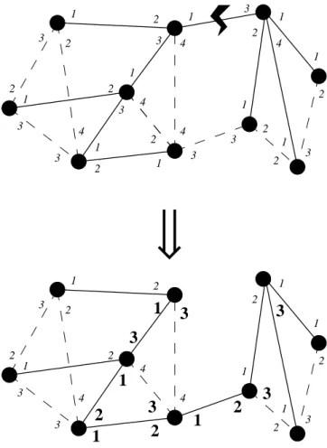
If edge e belongs to the spanning tree T , then T without edge e is not connected. Since we assume that the graph remains connected, there exists an edge e′in the new graph connecting the two parts of T . This edge e′ is added to the tree. Some port numbers have to be changed so that the local orientation become compatible with the resulting spanning tree. We claim that only a constant number of port numbers have to be modified at each node. At the extremities of e and e′, the set of tree-edges incident to it changes. However, at most two edges are concerned. Apart from this, the only modifications to do concern the choice of the incident edge with port number 1. A switch between two port numbers is sufficient. Therefore, at most a constant number of port numbers are modified at each node. An example is given in Figure 2.
• Removal of a leaf. Let v be the node connected to the removed leaf u. Let i be the port number at v of the edge leading to u. Let p be the largest port number at v of an edge in T. Let d be the degree of v before the removal of e. Finally, let e′, resp. e′′, be the edge incident to v with port number p, resp. d. Since edge e is in the tree T , we have i ≤ p ≤ d. We modify the port number of e′, resp. e′′, if and only if i 6= p, resp. p 6= d. If i 6= p, then we set i as the new port number of e′. If p 6= d, then we set p as the new port number of e′′. In all cases, the other port numbers in the graph remain inchanged.
It may not be possible to avoid a linear number of modifications in the case of the removal of a tree-edge. For example, consider a cycle C of odd length 2n + 1. To simplify the description, let us give names from 1 to 2n + 1 to the nodes. For any node i ≤ n, resp. i > n, 1 is the port number of the edge leading to node i + 1, resp. i − 1. Thus the local orientation is compatible with the path starting at node 1 and ending at node 2n + 1. Now assume that the edge {n, n + 1} is removed. The port numbers at node n and n + 1 are set to 1 since they are now leaves. All edges are necessarily in the spanning tree but the edge {2n + 1, 0} has both its port numbers equal to 2. The local orientation is not tree-oriented. In fact, in a tree-oriented orientation, exactly one edge emust have both its port numbers equal to 1. Moreover, for any node v, excluding the extremities of e, the edge with port number 1 must point toward e, i.e., the edge must be in the path from v to the closer extremity of e. Hence, the local orientation has to be modified in at least n nodes to
1 1 1 1 1 1 4 2 4 2 2 3 2 2 2 3 3 3 4 2 1 1 1 1 1 1 1 1 1 1 4 4 2 3 2 2 3 2 4 3 4 2 2 3 2 3 2 2 3 3 3 4 2 3
1
2
3
1
2
3
3
3
1
3
1
2
Figure 2: Removal of an edge belonging to the spanning tree.
Plain lines represent edges of the spanning tree. Bold numbers represent port numbers modified by our algorithm to preserve the tree-oriented property.
4
Further Investigations
In this paper, we proved the upper bound 4n − 2 on the minimal period π(n) for periodic graph exploration by a finite automaton. Since graphs are anonymous, using an extensive amount of memory does not help much. Therefore finding the minimal period for machine with unbounded memory may be very challenging.
Open problem. What is the mimimum period ψ(n) such that there exists an algorithm setting the local orientations and a robot with unlimited memory such that the robot explores any graph of size n within the period ψ(n)?
Finally, it remains open if the period 10n proved in [11] can be improved if the robot is restricted to be oblivious.
References
[1] Y. Afek and E. Gafni. Distributed Algorithms for Unidirectional Networks. SIAM J. Com-puting 23(6):1152-1178, 1994.
[2] S. Albers and M. R. Henzinger. Exploring unknown environments. SIAM J. Computing 29:1164-1188, 2000.
[3] D. Avis and K. Fukuda. Reverse search for enumeration. Discrete Appl. Math, 65(1-3):21-46, 1996.
[4] M. Bender, A. Fernandez, D. Ron, A. Sahai and S. Vadhan. The power of a pebble: Exploring and mapping directed graphs. Information and Computation 176(1):1-21, 2002.
[5] L. Budach. Automata and labyrinths. Math. Nachrichten, pages 195-282, 1978.
[6] R. Cohen, P. Fraigniaud, D. Ilcinkas, A. Korman and D. Peleg. Label-Guided Graph Explo-ration by a Finite Automaton. In 32nd Int. Colloq. on Automata, Languages & Prog. (ICALP), LNCS 3580, pages 335-346, 2005.
[7] S. Cook and C. Rackoff. Space lower bounds for maze threadability on restricted machines. SIAM J. on Computing 9(3):636–652, 1980.
[8] S. Das, P. Flocchini, A. Nayak, and N. Santoro. Distributed Exploration of an Unknown Graph. In 12th Colloquium on Structural Information and Communication Complexity (SIROCCO), LNCS 3499, pages 99-114, 2005.
[9] X. Deng and C. H. Papadimitriou. Exploring an unknown graph. J. Graph Theory 32(3):265-297, 1999.
[10] K. Diks, P. Fraigniaud, E. Kranakis, and A. Pelc. Tree Exploration with Little Memory. J. Algorithms 51(1):38-63, 2004.
[11] S. Dobrev, J. Jansson, K. Sadakane, and W.-K. Sung. Finding Short Right-Hand-on-the-Wall Walks in Graphs. In 12th Colloquium on Structural Information and Communication Complexity (SIROCCO), LNCS 3499, pages 127-139, 2005.
[12] G. Dudek, M. Jenkin, E. Milios, and D. Wilkes. Robotic Exploration as Graph Construction. IEEE Transaction on Robotics and Automation 7(6):859-865, 1991.
[13] C. Duncan, S. Kobourov, and V. Kumar. Optimal constrained graph exploration. In 12th Ann. ACM-SIAM Symp. on Discrete Algorithms (SODA), pages 807-814, 2001.
[14] R. Fleischer and G. Trippen. Exploring an unknown graph efficiently. In 13th Annual Inter-national Symposium on Algorithms (ESA), LNCS 3669, pages 11-22, 2005.
[15] P. Flocchini, B. Mans, and N. Santoro. Sense of direction in distributed computing. Theoretical Computer Science 291(1):29-53, 2003.
[16] P. Fraigniaud, L. Gasieniec, D. Kowalski, and A. Pelc. Collective Tree Exploration. In 6th Latin American Theoretical Informatics (LATIN), LNCS 2976, pages 141-151, 2004.
[17] P. Fraigniaud, C. Gavoille, and B. Mans. Interval routing schemes allow broadcasting with linear message-complexity. Distributed Computing 14(4):217-229, 2001.
[18] P. Fraigniaud, and D. Ilcinkas. Digraphs Exploration with Little Memory. In 21st Symposium on Theoretical Aspects of Computer Science (STACS), LNCS 1996, pages 246-257, 2004. [19] P. Fraigniaud, D. Ilcinkas, G. Peer, A. Pelc, and D. Peleg. Graph Exploration by a Finite
Automaton. In 29th International Symposium on Mathematical Foundations of Computer Science (MFCS), LNCS 3153, pages 451-462, 2004.
[20] A. Hemmerling. Labyrinth Problems: Labyrinth-Searching Abilities of Automata. Volume 114 of Teubner-Texte zur Mathematik. B. G. Teubner Verlagsgesellschaft, Leipzig, 1989.
[21] P. Panaite and A. Pelc. Exploring unknown undirected graphs. J. Algorithms 33(2):281-295, 1999.
[22] N. Rao, S. Kareti, W. Shi, and S. Iyengar. Robot navigation in unknown terrains: Introductory survey of non-heuristic algorithms. Tech. Report ORNL/TM-12410, Oak Ridge National Lab., 1993.
[23] O. Reingold. Undirected ST-Connectivity in Log-Space. In 37th ACM Symp. on Theory of Computing (STOC), pages 376-385, 2005.
[24] H. Rollik. Automaten in planaren Graphen. Acta Informatica 13:287-298, 1980 (also in LNCS 67, pages 266-275, 1979).