Computer simulation of the effects of a phosphorus plume on Ashumet Pond and associated remediation schemes

Computer Simulation of the Effects of a Phosphorus Plume on

Ashumet Pond and Associated Remediation Schemes

By

ENO'

Jeffrey W. Goulet

B.S., Civil and Environmental Engineering

Lehigh University, 1999

Submitted to the Department of Civil and Environmental Engineering in Partial

Fulfillment of the Requirements for the Degree

Master of Engineering

In Civil and Environmental Engineering

at the

Massachusetts Institute of Technology

June 2000

@ 2000 Jeffrey W. Goulet

All Rights Reserved.

The Author hereby grants to MIT permission to reproduce and to distribute publicly paper and electronic copies of this thesis document in whole or in part.

Signature of Autho

/

(~

Jeffrey W. Goulet

Department of Civil and Environmental Engineering

May

5,

2000

Certified by

Dr. E. Eric Adams

Senior Research Engineer and Lecturer

Thesis Supervisor

Accepted b_y

Computer Simulation of the Effects of a Phosphorus Plume on Ashumet Pond and

Associated Remediation Schemes

By

Jeffrey W. Goulet

Submitted to the Department of Civil and Environmental Engineering on May

5,

2000, in

partial fulfillment of the requirements for the degree of Master of Engineering in Civil

and Environmental Engineering

Abstract

Ashumet Pond is located southeast of the Massachusetts Military Reservation

(MMR) in the towns of Falmouth and Mashpee, Massachusetts. A sewage treatment

plant (STP) located inside of the MMR discharged phosphorus-rich treated sewage into

the ground for a period of approximately

50

years. As a result, a treated sewage plume

formed and has migrated a significant distance, intersecting Ashumet Pond in its

northwest corner.

Many studies have been done to try and assess the impact of the phosphorus-laden

groundwater on the pond. Over the last 20 years the pond has experienced heightened

levels of phosphorus inputs from the STP plume, and there is concern that this

phosphorus could cause excessive phytoplankton growth due to phosphorus being the

limiting nutrient.

The purpose of this study was to utilize a computer model to predict the

effectiveness of remediation schemes that have been proposed to control the amount of

phosphorus present in the water column. The model that was used in this study was the

Water Quality for River-Reservoir Systems (WQRRS), which was developed by the U.S.

Army Corps of Engineers. WQRRS is a one-dimensional model, and was used to

extensively model temperature profiles, dissolved oxygen, and phosphorus levels within

the water body.

The most promising remediation schemes that were proposed and modeled are

hypolimnetic extraction and sediment extraction. Both methods were found to be

effective in removing the phosphorus from the water column without causing large

disturbances in other ecological parameters. An attempt was made to model the

phytoplankton, but a lack of data prevented effective calibration.

Thesis Supervisor: Dr. E. Eric Adams

ACKNOWLEDGEMENTS

First, I would like to take this opportunity to thank Dr. Adams for his guidance

throughout this project, as well as the effort that he has put into the Meng program on a

whole.

Secondly, I would like to sincerely thank Peter Shanahan for his dedictation, patience,

and advice. Throughout the course of this project and the year he has been a tremendous

help and asset to the Meng program. Without him this project would not have been

possible.

Finally, I would like to thank all of my friends and family for believing in me and helping

me to achieve this goal. I would especially like to thank my parents Wayne and Linda,

my brothers Bruce, Paul, and Shaun, and my grandparents. Without all of your help and

support, I could never have achieved this!!

TABLE OF CONTENTS

List of Figures...

6

List of Tables ...

...

8

1

Introduction...

9

1.1 PROBLEM STATEMENT ...

9

1.2 SITE LOCATION AND HISTORY...

9

1.3 ASHUMET POND ... 10

1.4 BACKGROUND ON THE ASHUMET VALLEY PLUME ... 12

1.5 W ATER QUALITY DYNAMICS ... 14

1.6 EUTROPHICATION... 18

1.6.1

Carbon Cycling ...

20

1.6.2

Nitrogen Cycling ...

20

1.6.3 Phosphorus Cycling ...

20

1.6.4 Limiting Nutrient ...

20

2

Trophic State Analysis ...

22

2.1 TROPHIC STATE ... 22

2.2

22

2.3 NYSDEC CRITERIA ... 24

3

Computer Modeling of Ashumet Pond...25

3.1

3.2

31

3.2.1

Inflows to Ashumet Pond...

32

3.2.1.1 Phosphorus Budget in Ashumet Pond...33

3.2.1.2 Other Constituents...

38

3.2.2

Outflows ...

39

3.2.3

Calibration ...

39

3.2.3.1 W ater Budget...

40

3.2.3.2 Thermal Profile...

40

3.2.3.3 Dissolved Oxygen Concentration...

45

3.2.3.4 Phosphorus Concentration...48

3.2.3.5 Phytoplankton and Zooplankton ...

51

4

Possible Rem ediation Schem es...52

4.1 CONTROLLING THE EXTERNAL PHOSPHORUS LOAD ...

52

4.1.1

Pump and Treat ...

52

4.1.2 Hydraulic Diversion ...

53

4.1.3 Monitored Natural Attenuation...

53

4.2 IN-LAKE CONTROL OF PHOSPHORUS...53

4.2.1 Nutrient Inactivation ...

54

4.2.2 Ferrous Iron Addition ...

54

4.2.4 Circulation ...

57

4.2.5 Oxidation of Sediments...

57

4.2.6 Biomanipulation ...

58

4.2.7 Sediment Removal ...

58

4.2.8 Hypolimnetic Withdrawal ...

59

5

Testing the Possible Remediation Schemes...

60

5.1 HYPOLIMNETIC WITHDRAWAL ...

60

5.2

5.3

6

Conclusions and Recommendations ...

68

6.1

68

6.2 RECOMMENDATIONS ... 69

7

Bibliography ...

71

List of and Figures

Figure 1.1 Ashumet Pond's Bathymetry Figure 1.2 Ashumet Vally Plume

Figure 1.3 Field Data of Temperatures at Different Depths Figure 1.4 Field Data of Dissolved Oxygen at Different Depths

Figure 1.5 Field Data of Phosphorus Concentrations at Different Depths

Figure 3.1 A Geometric Representation of the Reservoir and Mass Transport Mechanisms Used by WQRRS

Figure 3.2 Interaction of Constituents within WQRRS Figure 3.3 Phosphorus Budget Within Ashumet Pond

Figure 3.4 Phosphorus Concentration in the Groundwater Entering in to Ashumet Pond Figure 3.5 Graphical Representation of the Sources and Sinks of Phosphorus in Ashumet

Pond

Figure 3.6 Comparison of Experimental and Model Predictied Temperature Profiles in July 1999

Figure 3.7 Comparison of Experimental and Model Predicted Temperature Profiles in August 1999

Figure 3.8 Comparison of Experiemental and Model Prediceted Temperature Profiles in September 1999

Figure 3.9 Comparison of Temperatures at the MMR and Logan Airport

Figure 3.10 Comparison of Experimental and Model Predicted Profiles in August 1993 Figure 3.11 Comparison of Experimental and Model Predicted Profiles in June 1994 Figure 3.12 Comparison of Experimental and Model Predicted Dissolved Oxygen in July

1999

Figure 3.13 Comparison of Experimental and Model Predicted Dissolved Oxygen in August 1999

Figure 3.14 Comparison of Experimental and Model Predicted Dissolved Oxygen in September 1999

Figure 3.15 Comparison of Experimental and Model Predicted Dissolved Oxygen in August 1993

Figure 3.16 Comparison of Experimental and Model Predicted Dissolved Oxygen in June 1994

Figure 3.17 Comparison of Experimental and Model Predicted Phosphorus Concentrations in July 1999

Figure 3.18 Comparison of Experimental and Model Predicted Phosphorus Concentrations in August 1999

Figure 3.19 Comparison of Experimental and Model Predicted Phosphorus Concentrations in September 1999

Figure 4.1 Phosphorus Concentration Contours

Figure 5.1 Model Predicted Effects of Hypoplimnetic Extraction at 7 liters/sec on August 17, 1999

Figure 5.2 Model Predicted Effects of Hypoplimnetic Extraction at 7 liters/sec on September 27, 1999

Figure 5.3 Model Predicted Effects of Hypoplimnetic Extraction at 28 liters/sec on September 27, 1999

Figure 5.4 Model Predicted Effects of Sediment Extraction on September 27, 1999 Figure 5.5 Model Predicted Effects of Pumping and Treating on September 27, 1999

List of Tables

Table 2.1 Range of Data and Average Values Table 2.2 Calculated TSI Values and Ranges Table 2.3 NYSDEC Trophic State Criteria Table 3.1 Ashumet Pond Phosphorus Budget

Table 3.2 Past Estimates of Ashumet Pond Phosphorus Budget Table 3.3 Concentration of Constituents Modeled in the Inflow

1 Introduction

1.1

Problem Statement

Over the past 20 years Ashumet Pond has been studied extensively to monitor the possible deterioration of the water quality due to phosphorus in the Ashumet Valley Plume, which originated inside the Massachusetts Military Reservation (MMR) boundary. The pond is in danger of experiencing excess algae growth, which would severely reduce the ponds usefulness as a recreational area for boating, fishing, and swimming. This study was done to assess the phosphorus loading within the pond and to use a computer model to simulate remediation techniques that have been proposed to reduce the phosphorus concentration in the pond.

1.2 Site Location and History

The MMR is located in Barnstable County, Massachusetts, in the western portion of Cape Cod known as the "upper Cape". It is comprised of about 22,000 acres, within the towns of Bourne, Falmouth, Mashpee, and Sandwich (Jacobs Engineering, 1999).

The MMR site has played host to numerous sectors of the United States Military since its beginning as a training ground for the Massachusetts National Guard in 1911. In the 1920s and early 30s, the reservation had private owners, but was bought by the government and transformed into a National Guard training camp in 1935. World War II marked the peak in military activity at MMR. The war effort spawned tremendous growth within the facility as over 1400 buildings were built, and over 50,000 people were assigned to the training camp at that time in preparation for war (Rolbein, 1995)

The airfield became active in 1941, and facilitated coastal surveillance. The site was also conducive to several forms of special training, and troops practiced amphibious assaults on the beaches to prepare for similar attacks in Asia, Africa, and throughout the Pacific. Located on the base was the East Coast Processing Center, a facility dedicated to training reluctant patriots who

Following World War II, the MMR lease was reorganized several times among its occupants, primarily the Air Force, the Army, and the Coast Guard. The Commonwealth of Massachusetts currently leases MMR property to these parties. The 5,000-acre cantonment in the southern portion of the base has seen the most activity over the past century. It has been used by all three military branches and contains runways for airplanes, roads, housing, and maintenance facilities

for both aircraft and land vehicles (MMRIRP, 1996).

1.3 Ashumet Pond

Ashumet Pond has a surface area of approximately 203-acres and is described best as a kettle pond. Kettle ponds were formed at the end of the ice age as the glaciers receded. As the glaciers receded they left behind deposits of meltwater outwash that sometimes contained large ice blocks buried within (Wetzel, 1979). As the ice blocks melted in the outwash, they created large depressions that are often very irregular in shape. This phenomenon explains the pond's irregular shape that consists of two deep depressions, one about 60 feet deep and the other about 20 feet deep. Figure 1.1 is a contour map of the pond's bathymetry.

Another interesting feature of Ashumet Pond is that it's primarily source of water is through groundwater recharge. The hydraulic gradient, or the direction of flow of the groundwater, is mainly in the north to south direction. It is estimated that 1/3 of the pond bottom accounts for groundwater inflow, while the remaining 2/3 is groundwater outflow. The "hinge line," also in Figure 1.1, shows the approximate boundary between groundwater inflow and outflow. Other sources of inflows to the pond are the 180- 200 acre watershed consisting wooded, residential, and beach areas, a cranberry bog that has seasonal inflows of water, and direct precipitation (E.C. Jordan Co., 1988).

JOHNS POND

Legend

~-~-Water

MSL Mean Sea Level

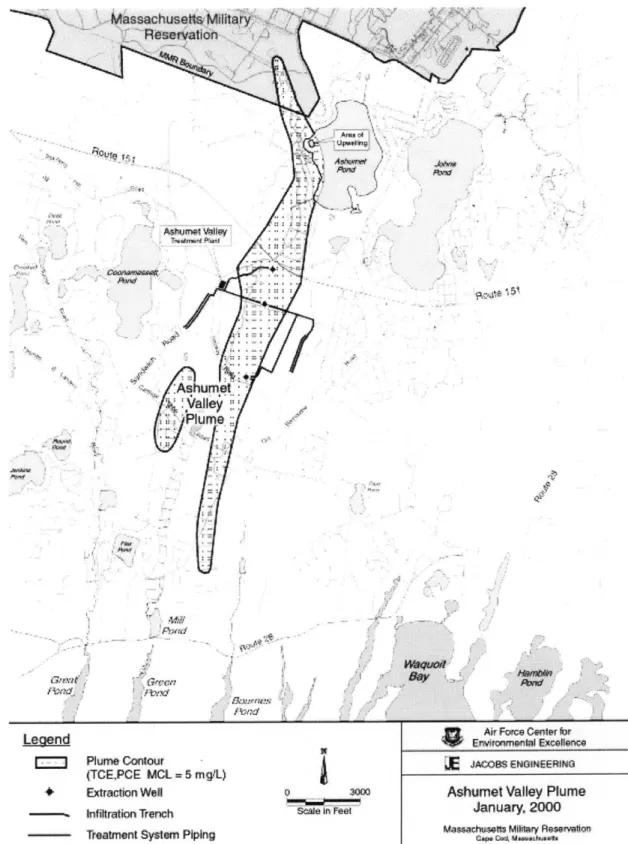
1.4 Background on the Ashumet Valley Plume

The Ashumet Valley Plume was formed from the discharge of treated sewage from a sewage treatment plant located just inside the southeast border of the MMR. The Sewage Treatment Plant (STP) was constructed in 1936 to treat approximately 0.9 million gallons per day (mgd) of sewage from the MMR. In 1941 the treatment plant was expanded to treat an average of 3 mgd and a maximum load of 6 mgd. Actual flows were much less than the design flows, and it is estimated that between 1936 and 1980, approximately eight billion gallons of sewage was treated at the plant (LeBlanc, 1984). A conservative estimate of 2 billion gallons of sewage was treated between 1980 and the closing in 1995 (Shanahan, 1996), bringing the total treated sewage to approximately 10 billions gallons.

The STP operated essentially unchanged from 1941 to 1995. The STP had primary treatment consisting of a comminutor with a bar screen, an aerated grease-removal unit, and Imhoff tanks. The secondary treatment system consisted of trickling filters and secondary settling tanks. The treated sewage was then discharged into 24 one-half-acre rectangular sand beds. Each bed was designed to handle the infiltration of 125,000 gallons per day (LeBlanc, 1984).

The STP plume was discovered in the 1970s when the Town of Falmouth had to terminate the use of a well 9,000 feet downgradient of the infiltration beds because of foaming due to surfactants in the plume. Other constituents of the STP plume are nitrogen, phosphorus, boron, dissolved organic carbon, and to a small extent volatile organic chemicals. The plume spread rapidly and to great extents due to the high hydraulic conductivity of the sandy soils. It is estimated that the hydraulic conductivity of the aquifer is 200 to 300 ft/d (LeBlanc, 1984), and this high conductivity has allowed the contamination to spread 24,000 feet downgradient from its origin, and to 4000 ft wide in some sections. Figure 1.2 shows the size and shape of the Ashumet Valley plume. The location of the former STP was at the northern tip of the plume.

II #tvfl 0/ 4bumelwdI& ndntfl P~M 4T ./ AVOW nat G"u MAY1 t~o 4 Pimattp

lw Air Fomce Center for

Leqend

4

Plume Contour - JcOXBS ENGINEEMaN

(TCE,PCE MCL = 5 mg/L)

* Extraction Well pS 30.00Ashumet Valley Plume -- Infiltration Trench Scale In Feet Jaua 20

Masachusefs MiKway Rsweton

Teatment System Piping uAP*.,,usM.avR,.

FIGURE 1.2 Ashumet Valley Plume (http://www.mmr.org/cleanup/maps)

reaching the pond (only 2,000 ft downgradient). The most probable explanation for this slow migration is the adsorption of phosphorus onto aquifer sediments and the formation of insoluble phosphorus compounds (LeBlanc, 1984). Metallic oxides, especially ferric hydroxide and aluminum and calcium hydroxides (Shanahan, 1996), are especially good at adsorbing phosphorus in groundwater. Lab experiments were conducted with native soils to try to determine the sorptive capacity. These lab experiments involved exposing the native soils to extremely high initial concentrations of phosphorus, and then monitoring the sorption. Two sorption reaction rates were found. The initial sorption reaction that occurs is rapid and is followed by a slower reaction usually lasting a total of 12 to 15 days. When tests were conducted with initial concentrations representative of the actual treated sewage, the sorption was rapid and completed in about 24 hours. As a result it was concluded that the soils in the aquifer should have capacity to sorb all of the dissolved phosphorus released from the STP (Walter et al., 1996). However, since the treated sewage was released into the aquifer for over 50 years, available sorption sites have become occupied, which has allowed the phosphorus to migrate downgradient. This migration, however, has been at a very slow rate compared to the rest of the plume. Since the STP has ceased operation, uncontaminated groundwater has begun to flush the plume, and phosphorus is predicted to slowly desorb and migrate downgradient.

Studies have shown that pockets of phosphorus exist in the plume where concentrations are in excess of 6 mg P/L, while the average uncontaminated groundwater in the aquifer is only .05 mg P/L (Shanahan, 1996). The most recent studies show that these pockets have reached Ashumet pond, and in fact may have been contributing to the phosphorus budget for some time.

1.5 Water Quality Dynamics

In order to understand the problems that are affecting Ashumet Pond, one must have an elementary knowledge of water quality dynamics. In most deep quiescent ponds a condition known as stratification occurs. Stratification refers to a separation in a water body due to density differences. The basic physical process that drives stratification is that more dense water sinks, while less dense water rises. Changes in density can occur from differences in the salinity or temperature of the water. Colder water generally is denser than warm water, the densest water having a temperature of 4 'C. In the absence of high solar radiation, a water body usually remains well mixed as long as there is mixing from the wind or some other energy source. In

other words, there is sufficient movement within the water body to keep the temperature and other constituents within the water body well mixed.

Following the ice melt in the spring, Ashumet Pond is mostly uniform and well mixed by currents derived from the wind. As warm weather persists, the solar energy heats the surface waters and makes them less dense. Without deep currents and high wind velocities, the water body becomes very hard to mix completely and as a result stratifies, leaving the mixing between the layers to diffusion. Even slight differences in water densities make it very difficult to mix the entire pond. In the summer the pond can be characterized by having an upper layer that is generally warm, well mixed, and turbulent. This upper layer is referred to as the epilimnion. The deep, cold, and relatively unmixed region of the pond is referred to as the hypolimnion. The layer of water that lies in the middle of the hypolimnion and the epilimnion is called the metalimnion, which is characterized by its thermal gradient. When autumn approaches, the temperature falls in the atmosphere. The epilimnion loses the heat energy that it has gained over the summer months, and the density of the epilimnion ultimately becomes greater than that of the hypolimnion. The surface waters then sink and mix by convective currents or with a wind induced epilimnetic circulation. These mixing mechanisms then quickly eliminate the metalimnion until the entire volume of the lake participates in the mixing and circulation. This process, termed the fall turnover (Wetzel, 1975), is cyclical and occurs once a year.

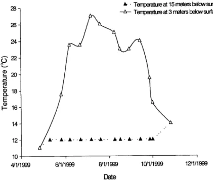
Figures 1.3, 1.4, and 1.5 show different characteristics of the pond in both the hypolimnetic and the epilimnetic regions over a period of stratification. The data was supplied by Jacobs Engineering (Jacobs Engineering, 2000a).

A Tempertureat 15meters below surface

-a- Temperasture at 3 rmters below surface

A-A. A-A-A-A.A A -A- -A-A

61/1999 8/1/1999 10(1/1999 12/1/1999

DEte

FIGURE 1.3 Field Data of Temperatures at Different Depths

-a Dissolved Oxygen 15 meters below surface -- Dissolved Oxygen 3 meters below surface

- . U U -.. 6/1/1999 U E* EU- E**E ~ 8/1/1999 10/1/1999 12/1/1999 Date

FIGURE 1.4 Field Data of Dissolved Oxygen at Different Depths

24-M

1000

-.*

- Phosphate Levels 15 meters below surface 800 --- Phosphate levels 3 meters below surface -'

600 -0 CZ 400 200 0 -4/1/1999 6/1/1999 8/1/1999 10/1/1999 12/1/1999 Date

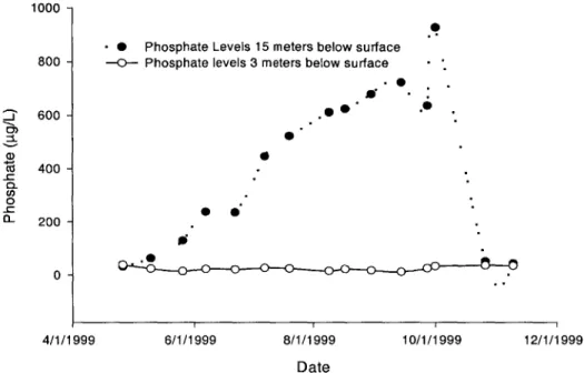
FIGURE 1.5 Field Data of Phosphorus Concentrations at Different Depths

The previous figures graphically depict the stratification cycle for temperature, phosphate, and dissolved oxygen in Ashumet Pond during 1999. Data collection began in late April, and ended in November. At the beginning of the collection period the pond was well mixed, characterized by similar values in the deep region and the shallow region of the pond. The pond then quickly became stratified, characterized by large differences in the temperature, dissolved oxygen, and phosphate values. In the beginning of October the fall turnover occurred, and the pond went back to being well mixed. The steep drop in dissolved oxygen in the hypolimnion is mainly due to the oxygen that is used during the decay of organic matter, and the fact that dissolved oxygen cannot be replenished in the hypolimnion due to the lack of mixing. Under anoxic, or oxygen depleted zones, there is a release of phosphorus from the sediments known as sediment regeneration. This release is clear in Figure 1.5. Under oxygenated conditions, phosphorus is often retained in the sediments at the bottom of the pond due to an oxidized microlayer at the sediment surface (Shanahan, 1996), but once this layer is depleted, phosphorus is liberated to the water column. Once conditions become oxygenated again, the microlayer forms and phosphorus gets trapped in the sediments.

1.6 Eutrophication

Extensive studies have been done over the last 20 years to determine if the STP plume emanating from the MMR has promoted eutrophication. Eutrophication traditionally refers to the natural aging process of a lake or pond where a water body becomes shallower and more productive through the introduction and cycling of nutrients. In a natural setting, a water body receives inflows of water from its surrounding watershed, direct precipitation, and groundwater. Along with the water, the water body also receives all the constituents that are in the water. These other constituents could include natural substances such as minerals and sediments, and they also could include man made substances that come from fertilizer runoff, septic system leakage, industrial waste, etc. As a result, the state of the water body reflects all the water and materials that flow in.

A lake or pond in its natural state is usually in a balance with the environment, resisting change in its trophic state. The trophic state is a term used to relate a water body's health to other water bodies, and also determines its stage of eutrophication. Inevitably a lake will become a marsh and ultimately a terrestrial system, but it is normal for a lake to remain in a trophic state for thousands of years.

There are three general trophic states in which a water body can be classified: oligotrophic, mesotrophic, and eutrophic. Oligotrophic water bodies are generally thought of as having low levels of nutrients, clear blue waters, and large depressions with steep sides (Home and Goldman, 1994). Because of the low levels of nutrients, there is a cascade effect up the food chain resulting in a relatively low level of fish and other biota. Oligotrophic lakes are often limited in phosphorus and have an abundance of nitrogen; therefore, the key constituent contributing to the eventual eutrophication of a lake is phosphorus (Wetzel, 1975). Eutrophic lakes, on the other hand, are very productive. They are usually less than 10 meters deep with gradually sloping edges and murky waters. Nutrients usually abound, making the water body very productive in terms of biological life. Mesotrophic lakes are the intermediates in the trophic status, and have characteristics of both oligotrophic and eutrophic water bodies. Water bodies in the mesotrophic state are the most common. Once a lake changes its trophic state it is almost impossible to change it back (Ryding and Rast, 1989). As a result, it is very important to the citizens of Falmouth and Mashpee to ensure that the trophic state of the pond does not change prematurely.

As previously mentioned, a eutrophic water body usually contains high levels of nutrients which promote algae growth. Algae require three macronutrients in order to grow: carbon, nitrogen, and phosphorus. Micronutrients may also be necessary in some cases. In order for uninhibited algae growth, all nutrients must be present but not necessarily in the same quantity. The average atomic ratio of the macronutrients necessary for growth is 106C: 16N: 1P, which is a simplified form of the Redfield ratio (Hemond and Fechner-Levy, 2000). If any of these nutrients are missing or not available in the necessary amount, algal growth becomes limited. This concept was formulated in 1840 by Justin Liebig, who claimed that, "growth of a plant is dependent on the amount of foodstuff that is presented to it in minimum quantity." Today this concept is known as Liebig's law of the minimum. Liebig's law, however, only applies if the actual cause of limited growth is nutrient related, and not due to lack of sunlight or sub-optimal temperatures (Ryding and Rast, 1989).

Mass is normally recycled in an ecosystem. Chemical substances generally are passed from one trophic level to another via the food chain, starting with the smallest plants, which are algae. Eventually the carbon and other nutrients cease to move up the food chain and are put back in the water column in the form of detritus, which is comprised of dead organisms or excretion.

As the detritus sinks to the bottom of the water column it begins to undergo mineralization, which is the process by which microbes convert organic compounds back to their inorganic forms. Mineralization occurs as the result of redox reactions in which electrons are transferred from one atom to another through the use of an electron acceptor. During this transfer there is an energy release to the microbes that allows them to live. The size of the energy release is dependant on the electron acceptor that is used; therefore, electron acceptors are usually utilized in a specific order. Oxygen is the electron acceptor that releases the most energy, followed by nitrogen, magnesium, iron, and sulfate. As a result, the microbes that can use oxygen as a substrate often dominate in a water body until the oxygen has been depleted, then microbes favoring nitrogen take over, and so on until all of the sulfate has been used up in a system. Following the depletion of sulfate, organic material decomposes by fermentation in a process called methanogenesis, in which methane gas is produced (Hemond and Fechner, 1994).

1.6.1 Carbon Cycling

Almost all algae receive their carbon from dissolved carbon dioxide that is found in water. The carbon dioxide has a constant source of replenishment from the air. When the algae dies or is consumed by another living organism the organic carbon is mineralized back to carbon dioxide thus completing the carbon cycle.

1.6.2 Nitrogen Cycling

In most water bodies nitrogen is introduced in the form of nitrate, which the algae can immediately use as substrate. As the algae die and begin to decompose, nitrogen is released in the form of ammonia. The ammonia then undergoes a process called nitrification, where it is oxidized back to the nitrate form. The previously described cycle occurs under aerobic conditions. Under anaerobic conditions, such as within the sediments, nitrate is further reduced by bacteria to nitrogen gas in a process called denitrification. The nitrogen is then generally lost from the system. However, a few species of algae do have the capability to convert nitrogen gas from the atmosphere to organic nitrogen.

1.6.3 Phosphorus Cycling

Most phosphorus that is found in water bodies originates from external sources. In most cases phosphorus must be in the inorganic form of orthophosphate in order to be used by algae and incorporated into organic compounds. As organisms die, they sink to the pond bottom where they decay and mineralize. During mineralization phosphorus is released, but often becomes retained in the sediments due to the oxidized micro layer described in Section 1.5. Phosphorus sediment regeneration may not be harmful during periods of stratification when there is not complete mixing in the water body, but when the water body has its fall overturn the phosphorus will be spread throughout the pond (Davis and Cornwell, 1998).

1.6.4 Limiting Nutrient

As described above, phosphorus is the only nutrient that is not readily available in the atmosphere and must originate from sources outside of the water body. As a result, phosphorus is usually

deemed the limiting nutrient in most fresh water bodies. However, one must be careful when investigating eutrophication problems because it is not uncommon that a water body is controlled by the amount of nitrogen in the ecosystem (Davis and Cornwell, 1998). Even if a water body is labeled as "nitrogen" or "phosphorus" limited, different species use nutrients in different ratios and have affinities for different types of nitrogen and phosphorus. This makes it difficult to determine what the limiting factor actually is.

Because phosphorus can have such severe effects on water bodies, it is desirable and often necessary to limit the amount of phosphorus that is allowed to flow into a water body. The largest natural source of phosphorus comes from the weathering of rocks, which is very hard to control. Sources of phosphorus that can be controlled are the ones that man is responsible for, such as municipal and industrial wastewaters, seepage from septic tanks, and fertilizer runoff from agricultural practices. When man is responsible for promoting eutrophication, it is known as cultural eutrophication. Ashumet Pond is thought to be a victim of cultural eutrophication because a phosphorus flux occurs from a small stream coming from cranberry bogs to the north of the pond, residential septic systems which leach phosphorus into the pond, and most prominently the phosphorus rich sewage plume that originates in the MMR.

2 Trophic State Analysis

2.1

Trophic State

In order to assess the effects of the phosphorus plume on the pond, a trophic state analysis must be done to determine the pond's present state. None of the trophic states are absolutely defined, but rather water bodies are evaluated on an 'open boundary' classification system that rates the lake on certain chemical and biological criteria (Ryding and Rast, 1989). In other words, no fixed values are used to define a water body because a water body may be classified in one trophic state for one parameter and another trophic state for another parameter. Therefore, different parameters must be looked at and jointly evaluated to decide the final trophic state of a water body.

The basis for most trophic state indices is the relationship between phosphorus and chlorophyll-a. Chlorophyll-a is one of the green pigments that is involved in photosynthesis and is found in all algae. It can be a useful parameter to distinguish the amount of algae in the water apart from other organic solids such as bacteria.

Over the last 20 years Ashumet Pond has generally been classified as a mesotrophic water body by a variety of different classification methods. In the latest study conducted by Jacobs Engineering (Jacobs Engineering, 2000a-b), the pond seems to remain at the same trophic level, but may be bordering on eutrophic conditions.

2.2 Carlson's Trophic State Index

Carlson's Trophic State Index (TSI) (Carlson, 1977) is a popular trophic state indicator that is endorsed by the U.S. Environmental Protection Agency, but should only be used in lakes that have low non-algal turbidity and relatively few rooted plants. Ashumet Pond fits these criteria. The test utilizes three parameters to classify the system: the Secchi disk, chlorophyll-a, and phosphorus levels. A Secchi disk is a black and white disk that is lowered into a water body to measure the water's clarity. The disk is lowered into the water until it disappears, and then it is brought back up until it just reappears. The average depth is termed the Secchi depth.

Carlson's TSI uses a log transformation of the Secchi depth values to approximate algal biomass on a scale from 0-110. Phosphorus and chlorophyll-a are usually closely correlated with Secchi disk depth; therefore, they also can be used as indicators of trophic state using a log transformation. Equations 2.1, 2.2, and 2.3 show these transformations.

TSI = 60 - 14.41 In [Secchi depth (meters)] TSI = 9.81 In [Chlorophyll a (pg/L)] + 30.6 TSI = 14.42 In [Total phosphorus (pg/L)] + 4.15

(2.1) (2.2)

TSI = Carlson trophic state index In = natural logarithm

If a calculated TSI value falls in between 40 and 50, it is usually associated with mesotrophic conditions. Index values greater than 50 are associated with eutrophic conditions, and values less than 40 are associated with oligotrophic.

(http://www.epa.gov/ceiswebl/ceishome/atlas/ohiowaters/resources/moreaboutlakes.html)

Jacobs Engineering used the Carlson TSI method to determine the trophic state in its 1999 investigation (Jacobs Engineering, 1999). The range of data and average values for Secchi depth, total phosphorus, and chlorophyll-a are presented below in Table 2.1.

TABLE 2.1 Range of Data and Average Values (Jacobs Engineering, 2000a)

Secchi Depth (m) Total Phosphorus (gg/L) Chlorophyll a (gg/L)

Average 2.6 26 6.4

Range 1.6-5.5 18-43 1.5-19.2

TABLE 2.2 Calculated TSI Values and Ranges (Jacobs Engineering, 2000a)

TSI Value Trophic State

Secchi Depth 46 (35-53) Mesotrophic

Total phosphorus 51(46-58) Meso-Eutrophic

Chlorophyll-a 58 (44-69) Meso-Eutrophic

2.3 NYSDEC Criteria

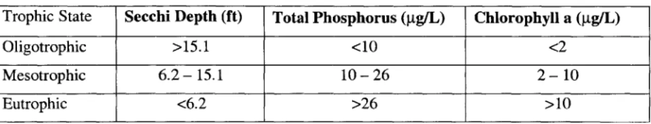
Jacobs Engineering also used the New York State Department of Environmental Conservation (NYSEC) criteria. Like Carlson's TSI criteria, the NYSDEC criteria assume that there is low non-algal turbidity and few rooted plants. The NYSDEC criteria base their determination of trophic state on the range of values in Table 2.3.

TABLE 2.3 NYSDEC Trophic State Criteria

Trophic State Secchi Depth (ft) Total Phosphorus (pg/L) Chlorophyll a (gg/L)

Oligotrophic >15.1 <10 <2

Mesotrophic 6.2- 15.1 10-26 2-10

Eutrophic <6.2 >26 >10

Using data from the 1999 Jacobs Engineering report, the NYSDEC criteria gives the pond a mesotrophic status for Secchi Depth and chlorophyll-a. The total phosphorus parameter lies on the border of mesotrophic and eutrophic.

In general Ashumet Pond appears to be mesotrophic, but bordering on eutrophic conditions. This new data correlates with earlier studies done by Shanahan in 1996 and E.C. Jordan in 1988 in which the pond was classified as mesotrophic.

3 Computer Modeling of Ashumet Pond

3.1 Water Quality for River-Reservoir Systems

The goal of modeling Ashumet Pond with a computer model was to represent and predict aspects of water quality within the pond. The software that was chosen to do this task was the Water Quality for River-Reservoir Systems, or WQRRS. WQRRS is a computer program that was developed by the US Army Corps of Engineer's Hydraulic Engineering Center (Smith, 1978). The program has the capability to model both the reservoir and river sections of a system; however, since Ashumet Pond does not have any river inflows, only the reservoir portion of the program was used.

WQRRS was chosen because it could effectively model the important water quality variables affecting Ashumet Pond. These main water quality variables are phosphorus content, phytoplankton, temperature stratification, dissolved oxygen content, and nitrogen content. The model is dimensional, represented by horizontal slices stacked on top of each other. A 1-dimensional model has the advantage of being simpler to use than a 2-1-dimensional or

3-dimensional model, but may not give accurate results in some water bodies due to turbulent mixing caused by surface water inflows and outflows. The model assumes that there is complete mixing within each slice, and internal transport of heat and mass happens only in the vertical direction. Figure 3.1 shows the geometric representation of the reservoir and mass transport mechanisms that are used by the model.

Evaporation

Tributary

Inflow

Tributary Inflow

Vertical Ad ection & Effective DXiffusio

Volume Element

Outf low

FIGURE 3.1 A Geometric Representation of the Reservoir and Mass Transport Mechanisms Used by WQRRS (Smith, 1978)

A theoretical method that can be used to determine if a 1-dimensional model is appropriate is the Froude number. If the calculated Froude number is much less than one, the water body is vertically stratified and applicable to WQRRS. If the Froude number is found to be much larger than 1, the pond is likely to have a horizontal gradient and could not be modeled using WQRRS. The Froude number can be calculated using Equation 3.1 (Orlob, 1969).

Froude =

LQ

Q

N = buoyancy frequency, sec-1

Ashumet Pond's Foude number was found to be about .00018, therefore the pond is vertically stratified and can be modeled using WQRRS.

The modeling approach that WQRRS uses is based on the concept of conservation of mass and energy, and can be used to model the dynamics of each chemical and biological component. The model uses Equation 3.2, below, to model the dynamics of thermal energy, biotic and abiotic materials:

ac = w ac D C. -C±S _(3.2)

at dz dz ' az A A

Where:

z = space coordinate, m w = vertical velocity, m/sec

Az = element surface area normal to direction of flow, m2 De = effective diffusion coefficient, m2/sec

qi = lateral inflow, m/sec

Ci = inflow thermal energy or constituent concentration in appropriate units gO = lateral outflow, m/sec

S = all sources and sinks in appropriate units, e.g., kcal/sec, mg/1/sec, etc.

Equation 3.2 is used for all constituents that move freely about a water body with the movement of the surrounding water. The constituents that can move freely (fish) are modeled using Equation 3.3 (Smith, 1978):

dc

- = ±S (3.3)

dt

Arguably, one of the most important parameters in a water body is the temperature because most chemical, biological, and even some physical parameters are temperature dependent.

Temperature changes occur because of transfer of heat to and from the air-water interface. Heat exchange with the sediments is ignored because the model assumes that the bottom area is small compared with the volume of the lake. Water surface heat exchange consists of five components:

qm = net rate of short-wave solar radiation across the interface

qm = net rate of atmospheric long-wave solar radiation across interface q = rate of long-wave radiation from the water surface

qe = rate of heat loss by evaporation

qc= rate of convective heat exchange between the water surface and overlying air mass

These five components are used in conjunction with the meteorological data to determine the heat flux to and from the water column. The meteorological parameters that are used to control the heat exchange coefficients are wind speed, dew point, dry bulb air temperature, and the fraction

of the sky that is cloud covered. Changes in these constituents are what drive the temperature profiles in the model.

The surface water temperature is also affected by adjusting the evaporation coefficients in the model. Increasing the evaporation coefficients lowers the temperature in the water, and decreasing the evaporation coefficients raises the temperature.

Once the energy is introduced to the water body, it is spread by the ponds hydrodynamics. WQRRS models the hydrodynamics in a pond using two types of net flow, advection and diffusion.

Advection is the bulk movement of fluid in a water body. WQRRS models advective mass transfer and heat within the system by algebraically summing the inflows and outflows, and then filling in the flow imbalances with vertical advection to the elements directly above and below a specified element. Figure 3.1 shows this process graphically with two tributaries contributing to the reservoir, one outflow, and the effects of evaporation. When there is an imbalance in the system, vertical advection occurs along with changing pond volumes.

Diffusion is the second process that is modeled, and is composed of molecular and turbulent diffusion as well as convective mixing. Wind and flow are usually responsible for diffusive mixing. In well-stratified reservoirs that do not contain large inflows, diffusive mixing can be a very important consideration, which is the case in Ashumet Pond. WQRRS allows the user to specify one of two methods for diffusive mixing. The first method is the wind method, which uses the wind as the main source of mixing. The second is the stability method, which assumes that mixing will be at a minimum when the density gradient is at a maximum. Since the pond is deep in some sections and well stratified with a strong density gradient, the stability method was found to be the most effective method for specifying diffusion. The stability method involves the use of effective diffusion coefficients and critical column stability to control the amount of diffusive mixing.

In order to model the biological constituents of a water body, WQRRS's ecological processes center around phytoplankton and its direct relationship with nutrients within the pond. Figure 3.2

option to either not use the parameter or hold the parameter constant at a specific value. However, when eliminating parameters in the model a user must be fairly certain that the parameters eliminated will not alter the outcome of the simulation. If they will alter the outcome, they should not be eliminated.

Aeration Bacterial Deday Chemical Equilibrium Excreta G Growth M Mortality P Photosynthesis R Respiration S Settling H Harvest

FIGURE 3.2 Interaction of Constituents within WQRRS (Smith, 1978)

A

B C

3.2

Modeling, Data, and Calibration

The modeling process involves three equally important steps: data input, calibration and validation, and predictions. The first two of these steps will be discussed in this chapter.

In order for the model to accurately predict results, accurate data must be input to the system, and the model must be calibrated to reflect the pond's specific characteristics. The compilation of accurate data to model Ashumet Pond is fairly straightforward, as there were extensive studies done on the pond in 1993, 1994, and 1999. The study done in 1999 has the most extensive data, having been collected on average once every two weeks. The data is inputted to WQRRS through a text file that must be formatted a certain way. The user manual written by Smith (Smith, 1978) gives a detailed description of how the text file must be set up. An example input file used during this study is presented in Appendix A of this document.

The WQRRS model runs by taking an initial set of conditions and parameters, and then predicting future conditions over a specified period of time. For best results it is recommended that the modeling begin during a time when there is no stratification. Ashumet Pond normally begins stratification in late April; therefore, the modeling began in April and ran through October. The remainder of the year was not modeled because of a lack of pond data before April and a lack of climatic data after October. Using WQRRS to model the pond year-round would also be erroneous because the model cannot account for ice cover that Ashumet Pond usually experiences in the winter months.

Jacobs Engineering performed the detailed study done on Ashumet pond in 1999. Data that was collected in April of 1999 was used for the initial conditions in the pond (Jacobs Engineering, 2000a). The Jacobs Engineering report was used to input initial conditions of temperature, dissolved oxygen, ammonia, nitrate, nitrite, and phosphate. Initial values for zooplankton and phytoplankton had to be estimated using past reports because the 1999 report did not include

these constituents.

observation, fraction of sky that was cloud covered, dry bulb air temperature, dew point, barometric pressure, and wind speed. In order to get the most accurate results, it is desirable to get the climatic data from a location close to the water body that is being modeled. There are many weather stations near the MMR that collect data; unfortunately none of them had complete records for the time periods that were needed. Therefore, climatic data from Logan airport, which is approximately 65 miles north of Ashumet Pond, was used.

Inflows and outflows from the pond are also extremely important. WQRRS is a model that was developed to model reservoirs that contain one or more tributary rivers. WQRRS models withdrawals through one or two wet wells that contain up to eight ports each, a flood control outlet, and an uncontrolled spillway that operates only when the total flow exceeds the combined capacity of the wet wells and flood control outlet. Because the inflows and outflows in Ashumet Pond are both done through groundwater, a few tricks had to be used to model the pond.

3.2.1 Inflows to Ashumet Pond

Modeling the tributary river as groundwater inflow was straightforward, but several assumptions had to be made. The assumption was that the water had a constant temperature throughout the entire modeling period of 14*C. This is a valid assumption because the temperature of groundwater generally remains constant throughout the year. A constant inflow rate is also specified, and is determined from a water budget of the entire pond. Because there is only one inflow source, the inflow must include not only the groundwater input, but also the precipitation that directly falls on the pond surface, intermittent flow from the cranberry bog, runoff from the immediate watershed, and storm water discharge (E.C. Jordan Co., 1988). On average the pond receives 3.5 x 106 m3/yr of water as inflow.

Another factor that is extremely important is the flux of other constituents into the pond, such as the dissolved oxygen, nitrate, nitrite, ammonia, and phosphate. Constituents such as phytoplankton and zooplankton do not exist in the groundwater or other sources of water, and therefore are not included in the inflows to the pond. The most important inflow constituent that is modeled in this study is the concentration of phosphate in the inflows. As a result, there have been numerous attempts to quantify the amount of phosphate that enters the pond on a yearly basis. Section 3.2.1.1 outlines phosphorus budget analysis that was done by Jacobs Engineering

(Jacobs Engineering, 2000a), but is typical of many of the analyses that have been done in the past.

3.2.1.1 Phosphorus Budget in Ashumet Pond

Normally phosphorus is not found naturally within a water body; therefore, all of the phosphorus that is present in a water body is assumed to have originated elsewhere. Ashumet Pond has a number of potential sources of phosphorus that could be damaging to the pond. The traditional sources of phosphorus used to develop Ashumet Pond phosphorus budgets are: groundwater impacted by the STP plume, groundwater not impacted by the STP plume, runoff from cranberry bogs, direct rainfall, residential septic systems, storm water runoff, and immediate watershed runoff. A significant source of phosphorus within the pond is regeneration from the pond sediments. There are only two significant phosphorus sinks within the pond, and they are sediment burial and groundwater outflow. Figure 3.3 graphically depicts the phosphorus budget within Ashumet Pond.

Total Precipitation Storm Water Discharge STP Plume Groundwater Inflows Surface Water Runoff Cranberry Bog Runoff

FIGURE 3.3 Phosphorus Budget Within Ashumet Pond

Sedimentation/Regeneration

Groundwater Outflow

00Sediment Burial

Phosphorus from the Groundwater

Phosphorus in the STP plume affects approximately 3% of the total groundwater inflow. This estimate was formulated according to recent studies done along the northwestern shore of Ashumet Pond known as Fisherman's Cove (see Figure 1.1). Figure 3.4 (Walter et al, 1996) shows the results of a study conducted by the US Geological Survey. The figure shows the location of the infiltration beds and the resulting contour lines of phosphorus concentrations. In some areas of the plume the phosphorus levels have peaked to levels greater than 6 mg/l; however, in the area of Fisherman's cove the phosphorus levels are generally 2 mg/L, which is still a high concentration when compared to the natural groundwater concentration of .026 mg/L.

70'32-50. 70*32'07"

Ba1e rom US. Gelogial surey agital data 0 500 1,000 2,000 FEET

1-24,000. 19_____lO,

U*Me~qe Timemae MemlC *00wdr

~

G ra ns v 0 250 50 METERS

FIGURE 3.4 Phosphorus Concentration in the Groundwater Entering into Ashumet Pond (Bussey and Walter, 1996)

Another source of phosphorus is septic tank discharges. Approximately 32 houses exist within 300 feet upgradient of the pond, and discharges from their septic systems could contribute to elevated concentrations of phosphorus as well.

In calculations done by Jacobs Engineering, it was found that the STP plume contributes approximately 42 to 82 kg/year of phosphorus to the pond. The rest of the groundwater, including the water contaminated by residential septic systems, contributes an additional 117 to

125 kg/yr of phosphorus.

Direct Surface Water Runoff

The watershed that directly drains into Ashumet Pond is fairly small, not to mention that a lot of the rainwater infiltrates into the sandy soil before it can run off. The phosphorus content of the surface water runoff is variable depending upon soil types, slopes, fertilization practices, and land use. A conservative estimate of the phosphorus contribution is found by using a watershed area of approximately 180 acres and a phosphorus concentration of .25 mg/L of phosphorus. These estimates result in a loading of approximately 6 kg/yr.

Storm Water Drainage

There are two major storm water drainage systems that flow into Ashumet Pond from the MMR. The storm drains are used primarily to drain the water from the airport runways, which are still in use at the MMR. No phosphate fertilizers are used in the grounds keeping activities around the areas of the storm drains (E.C. Jordan, 1988). The first storm drain discharges directly into Ashumet Pond, while the second discharges into the abandoned cranberry bogs. It is estimated that the storm drain that discharges directly into the pond is responsible for approximately 5 to 9 kg/yr of phosphorus to the pond.

Cranberry Bog

Abandoned cranberry bogs are located northeast of Ashumet Pond, and discharge runoff directly into the pond during certain times of the year. As previously mentioned, a storm drain from the

the pond, average phosphorus concentrations were found to be roughly .0035 mg/L, thus giving a total loading of approximately 2 kg/yr.

Precipitation

The final contributor to the phosphorus budget is from direct precipitation. The average phosphorus concentration in rainfall is estimated to be approximately .03 mg/l. Since the average annual rainfall is approximately 47.65 inches and the surface area of the pond is 203 acres, the phosphorus load is approximately 31.5 kg/yr.

Table 3.1 shows the phosphorus budget that was used to do the modeling. This budget is adapted from the Ashumet Pond Phosphorus Budget (Jacobs Engineering, 2000a).

TABLE 3.1 Ashumet Pond Phosphorus Budget

Water Inflow Phosphorus Phosphorus Percent of

Pond Budget Source (m3/yr) Concentration Flux (kg/yr) Total

Total Groundwater Inflow 4.7E+06 - 4.9E+06

STP Plume Groundwater Inflow 1.2E+05 - 1.6E+05 48-82 19.0 -39.0

Other Groundwater Inflow 4.5E+06 - 4.8E+06 .026 mg/L 117-125 46.0 -60.0 Storm Wwater Discharge 1.8E+04 - 3.7E+04 .25 mg/L 4.6-9.2 2.0 -4.0

Cranberry Bog Discharge 6.7E +05 .0035 mg/L 2.3 1

Surface Water Runoff 2.4E + 04 .25 mg/L 6 2.0 -3.0

Total Precipitation 9.9E + 05 .03 mg/L 30 12.0 - 14.0

Total 208-255

Regeneration 3759

Ashumet Pond Sink

Groundwater Outflow 4.9E+06 - 5.7E+06 216-239

Sediment Burial 69-84

1___ 1__ 284-322 1 1

Table 3.1 also shows regeneration within the pond. The regeneration is split into two entities, the first of which is regeneration within the water column. Regeneration within the water column measures the mineralization that takes place in the water, and is measured by the oxygen uptake in water samples. This value was then used to approximate the quantity of phosphorus regenerated within the water column. Based on the calculations done by Jacobs Engineering, approximately 3370 kg/yr of phosphorus is regenerated within the water column. Mineralization is part of the natural cycling of nutrients in the water column, and most of this phosphorus is used

as substrate. Sediment regeneration is the second term associated with regeneration. Sediment regeneration was described previously as the phosphorus that is released to the water column under anoxic conditions. The sediment regeneration was found to be approximately 390 kg/yr.

Phosphorus sinks are also shown in Table 3.1. The two main sinks are groundwater outflow and sediment burial, both of which are significant. From this study it appears that the sinks in the pond outweigh the sources if regeneration is not included. This imbalance may or may not be enough to counteract the inflows from the STP plume in the long run

Figures 3.5a and 3.5b are graphical representations of the phosphorus sources and sinks within Ashumet Pond. It is easy to see that the STP contributes a significant amount of the total phosphorus to the system, and if it was eliminated there would be significantly less phosphorus entering the pond annually.

-STP Plum Other Groundwater

-Storm Water

Ml Cranberry Bog

EM Sudao, Water Runoff

Direct Precipitation Groundwater Outflow Sediment Burial (a) FIGURE 3.5 (b)

Graphical Depiction of the Sources and Sinks of Phosphorus in Ashumet Pond a) Phosphorus Sources b) Phosphorus Sinks

In the past there have been other studies to derive an accurate phosphorus budget. Table 3.2 (Shanahan, 1996) shows some predicted phosphorus concentrations derived in past studies. It is clear that the loading that Jacobs Engineering calculated is higher than the predictions made in

Past Estimates of Ashumet Pond Phosphorus Budget (Shanahan, 1996)

3.2.1.2 Other Constituents

The remaining parameters necessary to model Ashumet Pond were all part of the nitrogen budget. Values of ammonia, nitrate, and nitrite were estimated using both the groundwater contribution and atmospheric contribution to the pond. Concentrations were derived for the groundwater using studies done by the United States Geological Survey (USGS) on the groundwater in the

immediate area. Table 3.3 shows the concentration of each constituent modeled in the inflows.

TABLE 3.3 Concentration of Constituents Modeled in the Inflow

Constituent Concentration (mg/)

Phosphate .073

Ammonia .07

Nitrate .10

Nitrite .11

Phosphorus Load Total Percentage Load Aerial Phosphorus Predicted

From STP Plume Phosphorus from MMR Plume Loading Rate Concentration Trophic State (kg/yr) Load (kg/yr) (%) (g/m2 - yr) ctig/L)

K-V Associates, 1991 37 126 30 0.15 17 Mesotrophic E.C. Jordan Co., 1988 Present, best ase 19 70 27 0.09 9 Oligotrophic Present, worst case 57 145 39 0.18 19 Mesotrophic Future, best case 187 241 78 0.29 32 Eutrophic Future, worst case 375 466 81 0.57 62 Hypereutrophic Walter et al., 1995 67 155 44 0.19 21 Mesotrophic Shanahan, 1996 205 293 70 0.36 39 Eutrophic No MMR -plume scenarios

Best case 0 51 0 0.06 7 Oligotrophic

Worst case 0 88 0 0.11 12 Mesotrophic

3.2.2 Outflows

As previously mentioned, outflows from the pond can be modeled using wet wells, an uncontrolled spillway, and a flood control gate. Simulation of the groundwater outflow can best be represented using one of the wet wells. A wet well is a device that can selectively withdraw water from different depths of a water body, and therefore was particularly useful in simulating groundwater inflows. One wet well was used, utilizing all 8 ports. Each port was spaced evenly at 2.5 meters, starting at an elevation of 1.25 meters above the bottom of the deep basin. Each port was set to extract water at the same rate. This even spacing and flow rate allowed for a reasonably good simulation of groundwater evenly flowing out at all depths of the pond.

One model assumption that should be mentioned is that, when the wet wells extract water from each level, they extract the water as well as all of the constituents in the water. This, however, may not be what is actually happening in the system. For example, phosphorus does not flow through the groundwater very well and therefore may not leave the pond at the rate specified. This may also hold true for algae and detritus that is suspended in the water column. Another assumption that could be pertinent is that the water is uniformly extracted in the model over all of the depths, when this may not be exactly representative of the real conditions in the pond. Both of these possible discrepancies had to be taken into account when analyzing the model and calibrating.

3.2.3 Calibration

Careful calibration of a model is equally important to getting accurate results as correct initial values. During calibration, parameters in the model are adjusted to reflect the actual conditions within a specific water body. WQRRS is programmed with an initial set of conditions relating to almost every physical and biological constituent within the pond, and a user is then responsible for making changes to these parameters to best represent the water body. As a result, calibration can be a tedious process and it is best achieved if it is done in an order where parameters that affect other parameters are calibrated first.