A computational study of a geometric embedding of minimum multiway cut

A. Computational Study of a Geometric

Embedding of Minimum Multiway Cut

by

David Shin

Submitted to the Department of Electrical Engineering and Computer

Science

in partial fulfillment of the requirements for the degree of

Master of Engineering in Electrial Engineering and Computer Science

at the

MASSACHUSETTS INSTITUTE OF TECHNOLOGY

May 2006

@ Massachusetts Institute of Technology 2006. All rights reserved.

A uthor ...

:... ... ... ... .

Department of Electrical Engineering and Computer Science

May 16, 2006

Certified by..,/..

....

.

...

...

As id

tR. Karger

Associate Professor

Thesis Supervisor

Accepted by ...

Chairman, Department Committee on Graduate Students

ARCHIVES

AUG 14 2006

LIBRAR IES

E.

S...rthur

C.

. Smith

rthur C.

Smith

A Computational Study of a Geometric Embedding of

Minimum Multiway Cut

by

David Shin

Submitted to the Department of Electrical Engineering and Computer Science on May 16, 2006, in partial fulfillment of the

requirements for the degree of

Master of Engineering in Electrial Engineering and Computer Science

Abstract

In the minimum multiway cut problem, the goal is to find a minimum cost set of edges whose removal disconnects a certain set of k distinguished vertices in a graph. The problem is MAX-SNP hard for k > 3. Cglinescu, Karloff, and Rabani gave a geomet-ric relaxation of the problem and a rounding scheme, to produce an approximation algorithm that has a performance guarantee of 3/2 - 1/k. In a subsequent study, Karger, Klein, Stein, Thorup, and Young discovered improved rounding schemes via computation experiments for various values of k, yielding approximation algorithms with improved performance guarantees. Their rounding scheme for k = 3 is prov-ably optimal (i.e., its performance guarantee is equal to the integrality gap of the relaxation), but their rounding schemes for k > 3 seemed unlikely to be optimal.

In the present work, we improve these rounding schemes for small values of k > 3, yielding improved approximation algorithms. These improvements were discovered by applying an improved analysis to the same set of computational experiments used by Karger et al. We also present computer-aided proofs of improved lower bounds on the integrality gap for various values of k > 3. For the k = 4 case, for instance, our work demonstrates a lower and upper bound of 1.1052 and 1.1494, respectively, improving upon the previously best known bounds of 1.0909 and 1.1539. Finally, we present additional computational experiments that may shed some light on the nature of the optimal rounding scheme for the k = 4 case.

Thesis Supervisor: David R. Karger Title: Associate Professor

Acknowledgments

I would like to thank my parents and my sister Sarah. Their support over the past years has been vital to me.

Dina Katabi and Dan Stratila allowed me to use their machines for my computa-tional experiments. I would like to thank them for their generosity.

Finally, I must thank David Karger for the many useful ideas and insights into this problem. I am grateful for his enthusiasm and advice.

Contents

2.1 The Geometric Relaxation of Calinescu, Karloff, and Rabani 2.1.1 The embedding . ...

2.1.2 The relaxation ... 2.1.3 Rounding schemes ... 2.1.4 Integrality gap ...

2.2 A Study of the Relaxation by Karger, Klein, 2.2.1 Density ...

2.2.2 Maximum density segments ... 2.2.3 Some important linear programs . 2.2.4 Side parallel cuts . ... 2.2.5 Computational experiments... 2.2.6 Results . ...

Stein, Thorup,

2.3 Additional Computational Experiments by Mlosk-Aoyama ... 3 R.evisiting the Linear Program of Karger et al.

3.1 The constraints of Karger et al. ... 7

3.2 Exact density bounds . . ... 3.3 Observations and results . ... 4 Lower Bounding the Integrality Gap

4.1 Preliminaries . . . ...

4.2 Finding exact minimum k-way cuts . ...

4.2.1 Branch and bound enumeration tree . . . . 4.2.2 Lower bounds . . ...

4.2.3 Branching order . . ... 4.2.4 Empirical performance ... 4.3 Searching for bad embedded graphs . ...

4.3.1 Grid graphs . . ...

4.3.2 General embedded graphs . ... 4.3.3 Results and Observations . ... 5 Study of Pair-Isolating Cuts

5.1 Interpreting Mosk-Aoyama's results . ... 5.2 An alternative approach ...

5.3 Experimental variations ... 5.4 Results and conjectures ...

6 Conclusion 6.1 Future work ... .. . . . 39 .. . . . 44 47 .. . . . 47 .. . . . . 48 .. . . . . 48 .. . . . 49 .. . . . . 50 .. . . . . 51 .. . . . . 52 . . . . . 52 .. . . . . 55 .. . . . . 56

List of Figures

2-1 Relationship between linear programs . ... ... 30

2-2 A pair-isolating slice ... ... . 34

3-1 A 1,2-conjugate pair of permutations. . ... ... 40

3-2 A 1,2-aligned segment, split into two parts . ... 42

3-3 Density contributions from a (1,2)-conjugate pair sub-distribution . 43 4-1 A graphical representation of a non-sparc cut . ... 59

5-1 An example of a non-binding constraint becoming a binding one upon addition of another constraint. ... ... . . . 66

List of Tables

2.1 The upper bounds on the integrality gap computed by Karger et al.. 33 3.1 The upper bounds on the integrality gap obtained by improving the

analysis of Karger et al ... .. ... .. . 45 4.1 Improved lower bounds on the integrality gap. .... . . . ... .. .. 57

Chapter 1

Introduction

In the minimum multiway cut problem, one is given a weighted graph and a size-k subset of the vertices called the terminals. The goal is to find a minimum cut whose removal disconnects the terminals from each other. The problem is MAX-SNP hard for k > 3, so we are interested in approximation algorithms.

We are particularly interested in a geometric relaxation of the problem formulated by Cl1inescu, Karloff, and Rabani. Their approach uses the common graph optimiza-tion technique of embedding a graph into a geometric space. In order to round this relaxed solution to a cut of the graph, one partitions the geometric space, as a parti-tioning of the geometric space naturally induces a cut in the graph. By partiparti-tioning the geometric space randomly according to a carefully chosen distribution, one can use the properties of the embedding to prove bounds on the expected value of the induced cut, thus generating an approximation algorithm.

Specifically, we have sought to investigate the integrality gap of this geometric relaxation. This value represents the best provable approximation factor based on Chlinescu et al.'s relaxation. The question has been resolved for the k = 3, but remains open for k > 3.

In the present work, we establish tighter lower and upper bounds on the exact value of the integrality gap for various values of k. Furthermore, we analyze some previous conjectures concerning the yet-to-be-discovered optimal rounding schemes for k > 3, while preselnting some conjectures of our own.

1.1

Problem Definition

We begin with some preliminary definitions and notation. Given a graph G = (V, E), and a nonnegative weight function w : E --+ R, a cut is a subset C C E, and the cost

of C is given by w(C) = E cc w(e). When we are additionally given a distinguished

subset T C V, we define a T-cut to be a cut whose removal disconnects every pair of vertices of T. In this context, the vertices of T are referred to as terminals. If k = ITI, we also call this type of cut a k-way cut of G.

In the minimum multiway cut problem, we are given as input G, w, and T, and seek to find a k-way cut of minimum cost. We notate the cost of the minimum k-way cut of a graph G by wo(G). Note that the minimum multiway cut problem is a natural generalization of the classical (s, t)-cut problem.

The minimum multiway cut problem arises in several applications. One may formulate the scheduling of jobs on multiple processors in distributed computing systems as a minimum multiway cut problem [11]. In computer vision, maximum a posteriori estimates of a certain useful class of Markov Random Fields can be obtained

by solving minimum multiway cut [2]. Other applications include partitioning files among the nodes of a network and partitioning the elements of a circuit during the design of electronic chips into the subcircuits that are placed on different chips [4].

1.2

Prior Work

The minimum multiway cut problem was first studied by Dahlaus, Johnson, Papadim-itriou, Seymour, and Yannakakis [4]. They showed that the problem was MAX-SNP hard for k > 3. Additionally, they gave a simple approximation algorithm: for each terminal, t, use the traditional minimum (s, t)-cut algorithm [5] as a subroutine to find the minimum cut separating t from the other terminals, and take the union of the k - 1 smallest such cuts. One can prove that this algorithm achieves an app)roxinlation factor of 2 - 2/k.

Calinescu, Karloff, and Rabani [3] then gave a novel geometric relaxation for the problem. Their idea was to embed the graph into the k-simplex, which is a (k - 1)-dimensional polytope in Rk with k vertices'. This embedding is done in such a way that the k terminals map to the k simplex vertices. Then, the simplex is partitioned into k regions, so that each vertex of the simplex lies in a different region. This partitioning, referred to as a k-way cut of the simplex, induces a k-way cut in the original graph in a natural way: an edge of the original graph is in the cut if its endpoints map to different regions of the partitioned simplex. The manner in which this partitioning is chosen (i.e., a probability distribution over k-way cuts of the simplex) is referred to as a cutting scheme. Calinescu et al. specify a simple cutting scheme and use the properties of the embedding to show that the resulting

approximation algorithm achieves a performance guarantee of 3/2 - 1/k.

Subsequently, Karger, Klein, Stein, Thorup, and Young [8] extended this work by developing cutting schemes for various values of k that yield improved approxima-tion ratios. These cutting schemes were found through computaapproxima-tional experiments involving probability distributions over a class of partitions of the simplex that they refer to as side-parallel cuts, abbreviated sparcs. They also gave a precise geometric criterion for proving the optimality of a cutting scheme. They then used this criterion to prove the optimality of their cutting scheme for the case k = 3, thus demonstrating the limits o:f the Calinescu et al. embedding for k = 3. The question of the optimal cutting scheme for k > 3, however, remained open.

Mosk-Aoyama, in his Master's thesis, considered alternatives to sparcs for the k = 4 case. He performed computational experiments involving a new class of partitions of the simplex. which he refers to as pair-isolating cuts. The results of his computational experiments led him to conjecture that no optimal rounding scheme for k > 3 can be defined purely in terms of sparcs.

1_{As illust.rIitive examplles, the 3-simplex is an equilateral triangle, and the 4-simplex is a regular}

1.3

Our Results

Our goal is to further understand the geometric relaxation of Calinescu et al. Specif-ically, we aim to establish tighter lower and upper bounds on the integrality gap of the relaxation for various values of k. The integrality gap represents the best approx-imation ratio one can prove using an analysis that bounds the optimum cut only by the value of the relaxation.

We were successful on both fronts. We found stronger upper bounds by applying a more careful analysis to the computational experiments of Karger et al. We found stronger lower bounds through an original set of computational experiments. For k = 4, we obtain bounds of 1.1052 and 1.1494, improving upon the corresponding Karger et al. bounds of 1.0909 and 1.1539. In the process, we devise a branch-and-bound heuristic algorithm to solve the minimum multiway cut problem exactly.

We also perform additional computational experiments for the k = 4 case to ex-plore the possible role of pair-isolating cuts in optimal cutting schemes. Our conjec-ture, on the basis of these additional experiments, is that an optimal cutting scheme can be defined without using pair-isolating cuts. A bolder conjecture is that an opti-mal cutting scheme can be defined purely in terms of sparcs.

1.4

Presentation Overview

In Chapter 2, we describe in detail the geometric embedding of Cilinescu et al., and the works of Karger et al. and Mosk-Aoyama. Chapter 3 discusses how we were able to tighten the analysis underlying Karger et al.'s computational experiments. The performance guarantees given at the end of Chapter 3 represent the best known values to date. In Chapter 4, we present our branch-and-bound heuristic algorithm to solve minimum multiway cut exactly, and show how we were able to use this algorithm to establish new lower bounds on the integrality gap of the relaxation. These bounds, given at the end of Chapter 4, also represent the best known values to date.

compu-tational experiments we have performed to investigate pair-isolating cuts. We believe these experiments to suggest that pair-isolating cuts are not a necessary component of the optimal cutting scheme. Concluding remarks and natural directions for future research are given in Chapter 6.

Chapter 2

Background

Our present work draws heavily upon the previous works of Calinescu et al., Karger et al., and Mosk-Aoyama. In this chapter, we introduce the key ideas and results of these previous works.

2.1

The Geometric Relaxation of ClMinescu, Karloff,

and Rabani

The basis of this work is the geometric relaxation of the minimum multiway cut prob-lem formulated by Calinescu et al. In order to lay the framework for this relaxation, we begin with some terminology and notation.

2.1.1

The embedding

The geometric space we consider is the k-simplex A = {x E RkIl - xi = 1 A x > 0}. Note that A is a polytope of Rk with k vertices. The i-th vertex is the point identified by the i-th coordinate vector e4, which has coordinates (e')i = 1 and (e')j = 0 for all j j i. To avoid ambiguity. we refer to the vertices of the graph, the elements of V,

as nodes, and reserve the word vertices for the vertices of the simplex.

We measure distance in the simplex by using the LI-norm divided byv 2. Thus, if x and y are points of the simplex, we have d(x, y) = E- xl• - yjI. If s is the

line segment in the simplex with endpoints x and y, we define the length of s to be

1s)

An embedding of a graph G - (V, E) into A is a mapping a : V --, A. For any e = (u, v) E E, we let a(e) denote the line segment connecting a(u) and a(v). We define the volume of a by

vol(a)

= w(e)|a(e)I.

eEE

Consider an embedding that maps each node to a vertex of the simplex, with the ith terminal mapping to the ith simplex vertex. Then each embedded edge has length

0 if its endpoints embed to the same vertex and 1 otherwise. Every such embedding naturally induces a k-way cut of the graph. In this context, the set of edges in the cut are the edges whose endpoints map to different vertices of the simplex. Thus, the volume of the embedding is equal to the value of the induced cut.

These observations motivate the following integer program formulation (IP) of the minimum multiway cut problem:

min vol(fl) s.t. 3 is an embedding into A

(IP)

P(u) E {e, e2 ,...,ek} Vu E V

fl(t) = et Vt E T

Here, we are assuming that the terminals are labeled 1, 2,.., k.

2.1.2

The relaxation

The integer problem is, of course, intractable, as it is equivalent to the original MAX-SNP hard mininmum nmultiway cut problem. However, by removing the integer

con-straints, we obtain a tractable linear programming relaxation (LP):

min vol(a) s.t.

a is an embedding into A (LP)

a(t)

= et

Vt E T

Expressing LP as a linear program is not trivial, as the objective function involves distances between embedded points. Distances are of the form d(x, y) = Ei

lxi - yiJ,

Ei

lxi

inequalities, which do not use absolute values:

d(x,y) Ž diZ(x,y) di(x, y) > xi - yi di(x, y) > yi - xi.

A feasible solution to LP is a mapping a from V to arbitrary points of A. We denote the optimal solution by a*. To convert a feasible solution a into a feasible solution 0 of IP, we partition the simplex into k regions, one per vertex of the simplex:

k

A =U Ri

s.t. ee

Ri Vi

i=1

We call such a partitioning a k-way cut of A. Our converted solution, 3, is such that /3(u) = e' iff a(u) C Ri.

With a k-way cut of A and a feasible solution a to LP, we can generate a feasible solution to IP, and thus a k-way cut of the original graph. Specifically, each region of the simplex generated by the k-way cut corresponds to a connected component of the graph after the cut edges are removed. This means that we add edge (u, v) to the

cut iff a(u) and a(v) lie in different regions of the simplex.

2.1.3

Rounding schemes

In order to turn this framework into an algorithm that finds k-way cuts of the graph, we must specify how to choose the k-way cut of the simplex. One option is to use randomized rounding by specifying a probability distribution over k-way cut of A. We call such a probability distribution a cutting scheme.

Note that a cutting scheme specifies how to "round" the solution of a fractional program (LP) to a solution of an integer program (IP). For this reason, we use the term rounding scheme interchangably with "partitioning scheme".

The rounding scheme used by Calinescu et al. is independent of the input graph. It has the property that the k-way cut of the graph induced by the random k-way cut has an expected cost at most 3/2 - 1/k times the volume of the computed embedding. The induced algorithm thus has an approximation ratio of 3/2 - 1/k.

2.1.4

Integrality gap

The approach of embedding-relaxation-rounding outlined thus far is a formulaic one, used throughout the literature to approximately solve many NP-hard graph opti-mization problems. In every such application of this methodology, the question of the value of the integrality gap of the relaxation arises.

Formally, in our framework, the integrality gap of the relaxation is the supremum, over all weighted graphs G, of the ratio of the minimum cost of any k-way cut of G divided by the volume of the minimum volume embedding of G. In other words, it is equal to the worst case ratio between the optimal value of the integer program IP and the optimal value of the linear program LP.

This value is significant as it represents the best approximation ratio one can prove using an analysis that bounds the value of the rounded solution only by the value of the relaxed solution.

2.2

_{A Study of the Relaxation by Karger, Klein,}

Stein, Thorup, and Young

The work of Karger et al. provides additional insight into the relaxation, as well as further results about its integrality gap. Among other things, they show that the problems of determining the integrality gap and finding a corresponding optimal rounding scheme can be expressed purely as a geometric question. Thus, the inte-grality gap and approximation ratio can be obtained by studying the simplex itself, without considering particular input graphs or embeddings.

2.2.1

Density

Let us say that a line segment s in A is cut by a k-way cut C if some region boundary of C intersects s. Let Ok(C, s) denote the number of times that C cuts s.

Given a probability distribution P over k-way cuts of A (i.e., a cutting scheme), and a line segment, s, in A, let the density of P on s be given by

rk(P,s) = ECEp [c(C s)]

We then define the maximum density of P, Tk(P), by

Tk(P) = sup 7k(P, s).

The supremum is taken over all segments s with endpoints in A. The relevance of Tk(P) is the following:

Lemma 1 (Karger et al.). A cutting scheme P yields a randomized approximation algorithm with approximation ratio at most Tk(P).

Proof. Let (a be the minimum cost embedding. Consider an edge e in G. This edge maps to a segment a(e), which is cut in expectation at most Tk(P, a(e)) -ja(e)j tinmes. By the Markov inequality, this upper bounds the probability that the edge is cut.

Thus, the expected cost of the induced k-way cut is at most

e e

=

k(P)vol(G).

Since LP is a relaxation of IP, the minimum volume lower bounds the minimum k-way

cut. The lemma follows. O

Lemma 1 suggests that we should search for cutting schemes P with the property that rk(P) is small. Thus, we define the minimum maximum density, k*, by

rk = infTrk(P), P

and frame our goal as finding the value of Tr. Here, the infimum is taken over all

probability distributions over k-way cuts. In fact, the work of Karger et al. indicates something stronger:

Theorem 2 (Karger et al.). There exists a cutting scheme whose maximum density equals the integrality gap. Thus, Tr equals the integrality gap.

The proof is highly technical and so we omit it here. The theorem is significant, as it implies that the value of 7r can be resolved exactly by the following twofold

strategy:

1. Find a family1 of cutting schemes {Pi} such that

lim Tk(Pi)= - .

i oo

2. Find a family of graphs, {Gi} such that

,iD-o vol(ac*(Gi)) = Tk "

1

0f course, if a single cutting scheme P could be found such that Tk(P) = r-, there would be no need to find an entire family. However, there is no guarantee that such a cutting scheme exists. Similar remarks apply for the fanily of graphs in 2.

Recall that Co(G) denotes the minimum k-way cut of G, and that a*(G) denotes an optimal embedding of G.

That the family of cutting schemes exists is implied directly by the definition of rT (with or without the theorem), but the existence of the family of graphs relies on the theorem. If the theorem were not true, it is unclear how one would identify a particular value as T(.

2.2.2

Maximum density segments

The work of Karger at al. demonstrates that the key property of a cutting scheme is the maximum density the cutting scheme has on any line segment in the simplex. Implicit in the work of Cllinescu et al. is the observation that it is only necessary to consider infinitesimal segments in certain orientations. This is captured by the following lemmas, which we will not prove.

Lemma 3. There is always a line segment of infinitesimal length that achieves the maximum density.

We say that a line segment is i, j-aligned if it is parallel to the edge whose endpoints are vertices i and

j

Lemma 4. There is always an aligned line segment that achieves the maximum den-sity.

These lemmnas simplify the task of computing -rk(P).

2.2.3

Some important linear programs

In this section, we introduce some linear programs that will be referred to extensively throughout this work.

Karger et al. noted that the problem of finding an optimal cutting scheme could be formulated as an infinite-dimensional linear program, with one variable for each k-way cut of the simplex, and one constraint for every infinitesimal aligned segment. The variables represent probabilities, thus inducing a cutting scheme, and each constraint bounds the density of the induced cutting scheme on the corresponding segment. The objective function minimizes the density bound. The solution to the linear program is an assigment of probabilities to the various k-way cuts, or a cutting scheme.

The linear program is as follows:

min

7-c= 1

SPC

(PRI-0o)

sup

Zpc

•

<

c s

Here, the sums are taken over the set of all k-way cuts C of the simplex.

Actually, a much more precise formulation is required, as the set of all k-way cuts is uncountable, making the sums in the constraints meaningless. The variables should rather take the form of a measure defined on some a-field of subsets of the set of all k-way cuts of the simplex, and the constraints should rather take the form of Lebesgue integrals2. Nevertheless, we present this (incorrectly formulated) infinite linear program for sake of simplicity. Throughout this work, we will only use dis-cretized versions of PRI-oo, for which an appropriate transformation from measures and Lebesgue integrals to discrete probability distributions and sums can be made.

In particular, the approach taken by Karger et al. was to partition a subset of the uncountably many k-way cuts into a finite collection of subsets,

Q.

sub-

distribution.

Furthermore, Karger et al. partitioned the simplex into a finite collection of cells, W, and observed that the supremum of PRI-oc could be taken over all segments s wholly contained in some cell W' E W (by Lemma 3). For any X C A, let S(X) denote the set of line segments whose endpoints lie in X. The linear program PRI-oo then becomes a legitimate one:

min -r 7

SPQ

_(PRI-oo

Q

sup EpQ -

(Q, s)

VW

E

W

sES(W) Q

The significance of this linear program is summarized by the following theorem. Theorem 5. The objective value of PRI-oo 2 is equal to the maximum density of the

cutting scheme specified by its variables.

Still, the suprema in the constraints represent an infinite number of constraints, making the linear program impractical, though legitimate. To get around this, let

0(Q,W)= sup Tk(Q,s),

sES(W)

and note that for any subset W C A,

sup pQ .-

rk(Q,

EPQ.

7k(Q,s)

EPQ -

seS(W) Q Q SES(W) Q

By computing an upper bound, O(Q, W), on 0(Q, W), for each Q E Q and W E

min T

E PO = 1

SQ

_(LP-UB)

PQ · '(Q, W) < 7 VW

C

Theorem 6. The objective value of LP- UB is an upper bound of the maximum density of the cutting scheme specified by its variables.

Remark 2.2.1. The two factors that can cause an optimal solution of LP-UB to be

non-optimal for PRI-oo2 are:

* The slack lost in the application of (2.1), and

* The gap between

O(Q,

W) and O(Q,

W).

The lower bounding linear program

In a similar fashion, the problem of finding a worst-case graph can be formulated as an infinite-dimensional linear program. By "worst-case graph", we mean a graph G for which the ratio (a) is maximal. Since the given ratio can only decrease by

replacing a* with a non-optimal embedding a, we can in fact formulate an infinite-dimensional linear program to find a worst-case embedded graph: that is, a graph G together with an embedding a for which the ratio wo(G) is maximal. Note that an embedded graph is simply a set of embedded nodes,

a(1),a(2),...,

our set of embedded nodes can be taken to equal the entire simplex, in which case the embedded graph can be fully expressed by an assignment of edge weights to simplex segments.

Thus, this infinite linear program has a variable for every segment of the simplex, and a constraint for every k-way cut of the simplex. The variables represent edge weights, and the constraints bound the cost of the mininmum k-way cut of the graph. One further constraint is used to set the volume of the embedding to 1, so that the quantity to be maximized is simply the cost of the mininum k-way cut of the graph. This can be done because the ratio is invariant under a scaling of the edge

3We may _{use a set (as opposed t.o a imultiset) of embedded nodes, since if two nodes embed to}

the same point of the simplex, they will never be separated by a. cut, allowing us to consider instead the graph formed by merging the two nodes into one.

weights. The objective function maximizes the cost of the minimum k-way cut of the graph.

The linear program is as follows:

max A

.

1

_(DUAL-oo)

inf

S

w>

A

The infimum is taken over all k-way cuts C of the simplex, and the sums are taken over all segments of the simplex. As before, the sums are meaningless as they are taken over uncountable sets, making this linear program formulation erroneous. Again, we point ouLt that we will only use discretized versions of DUAL-o, for which an appropriate transformation from measures and Lebesgue integrals to discrete weight assignments and sums can be made.

In particular, one natural approach is to consider a fixed embedding of a finite graph. We can do this by selecting a finite subset of points in the the simplex, V C A, and by defining a graph, G(V), whose vertices are the points of V, and whose edges are the elements of S(V). We let cuts(V) denote the set of k-way cuts of G(V). The infimum of DUAL-oo then becomes a minimum over a finite numbers of cuts. The linear program DUAL-oo then becomes

max

A

s

S(1)

_(LP-LB)

seS(V)

wS > A VC E cuts(V)

sEC

We call this linear program LP-LB, since the resultant value of A represents a lower bound on Ti, with the resultant {w₈} specifying an embedded graph that achieves that value. Unlike the linear program LP-UB, however, it is not clear that this linear program can be of imich Jpractical computational use, as the number of constraints is exponential in the size of the embedded graph. Karger et al. were able to bypass

PRI-oo dual D U A L -oo

discretize

PRI-OO2 discretize

slack

LP-UB ILP-LB

Figure 2-1: The relationship between the linear programs PRI-oo, PRI-oo2, DUAL-00, LP-UB, and LP-LB.

this difficulty for the k = 3 case by exploiting planarity to replace the exponentially many constraints with a provably equivalent set of polynomially many constraints.

One can see that this DUAL-oo is actually the dual of PRI-oo. This, along with strong duality, is in fact the key observation behind Theorem 2. The argument, however, requires some more rigor than what we have presented. Karger et al. take a more rigorous measure-theory based approach by considering finite discrete versions of both linear programs and by taking a limit as the discrete programs approach the given continuous ones.

The relationship between the linear programs PRI-oo, PRI-oo2, DUAL-oo,

LP-UB, and LP-LB are summarized by Figure 2-1.

2.2.4

Side parallel cuts

For small values of k, Karger et al. were able to solve instances of LP-UB using the linear program software CPLEX. In this section, we describe a particular type of cut they used in their set up. They refer to this type of cut as a side parallel cut, or sparc.

Define A,,= p = {x E A'x, = p} and Ax__p = {x E Axi >_ p} (similarly A,,<p).

Note that Azx=p is a hyperplane that runs through the simplex, parallel to the face opposite vertex i, at a distance p from that face. We call such a hyperplane a side parallel slice. This hyperplane cuts the simplex into two regions: the corner, Ax;:>p, and the base. A,,<p,.

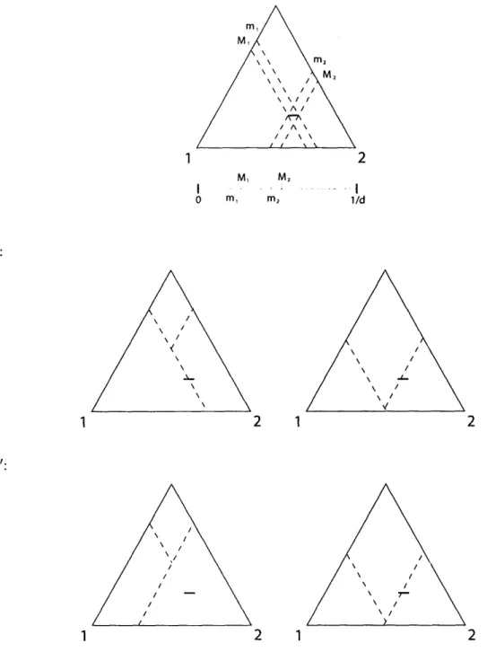
partition of A into regions 1, 2,..., k) resulting from the following procedure.

1. Choose a permutation a of the simplex vertices.

2. Process the vertices in the order specified by a. For each vertex i, except the last, choose a slice distance pi E [0, 1].

3. When vertex i is processed, assign to region i all the points in Ax>pi (the corner) that have not already been assigned to a previous region. We say that vertex i captures the points assigned to region i, and that it cuts a segment if it captures some of the points in the segment, but not the entire segment. 4. After the first (k - 1) vertices have been processed, assign the remaining

unas-signed points of the simplex to the final k-th region.

When a is chosen uniformly at random from the set of all permutations, and the slice distances are P1, p2,... , Pk-1, we call the resulting sparc a [P1, P2, ... Pk-1]-sparc.

2.2.5

Computational experiments

We can now describe the particular setup Karger et al. used for LP-UB. For their setup, they fixed an integer discretization level d, and used one sub-distribution for each element of {0, 1,..., d - 1}k-1_{. The sub-distribution for (ql, q}

2, ... ,q k-1) is

in-duced by choosing a value pi uniformly at random from [ql/d, (qi + 1)/dj for each i, and then by taking a [pl, 2, ... , Pk-1]-sparc. We refer to this specific sub-distribution as a sparc range.

For their cells, they used the regions of A formed by slicing the simplex along the hyperplanes xi = j/d for 1 < i < k and 1 <

j

{(X1, .-- ,Xk)

:

< x

1)/d}.

With this choice of cells and sub-distributions, a set of upper bounds Vp(Q, W) could be computed. Section 3.1 discusses how exactly Karger et al. computed these bounds. In Section 3.2, we will show how we were able to compute stronger bounds.

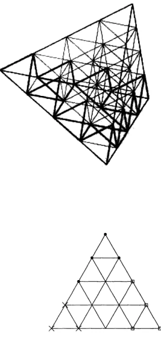
For the k = 3 case, Karger et al. were also able to solve instances of the linear program LP-LB for appropriately chosen embedded graphs. The embedded graph they used was chosen by fixing an integer discretization level d and by using all points in the simplex of the form (al/d, a2/d, a3/d) with al, a2, a3 E Z as embedded

nodes. Rather than listing the exponentially many constraints, however, they were able to rely on max-flow/min-cut duality and the planarity of the simplex to devise an equivalent linear program with only polynomially many constraints. They could not use an analogous strategy for k > 3, and so were unable to obtain better lower bounds on 7- for k > 3.

2.2.6

Results

For the k = 3 case, Karger et al. were able to observe convergent behavior for the solutions of both LP-UB and LP-LB as the discretization level increased. This led to the following discoveries:

1. A cutting scheme P for which they could prove analytically that T3(P) = 12/11.

2. A family of embedded graphs, {aj(Gi)} such that

lim wo(G%) 12

i- -oo vol(oai(Gi))9

11-These discoveries together imply that T3 = 12/11.

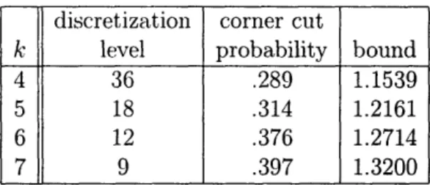
For greater values of k, solutions to LP-UB led to computer generated proofs of upper bounds for T-. These values are summarized in Table 2.1. Their experiments revealed an interesting fact: in all cases, the optimum cut distribution made use of '"corner cuts." That is, the output distribution had the following form: with some probability, place each slice at a single distance chosen uniformly between 0 and 1/3 from its terminal; otherwise, use a (joint) distribution that places each slice at distance greater than 1/3 from its terminal.

discretization corner cut

k level probability bound

4 36 .289 1.1539

5 18 .314 1.2161

6 12 .376 1.2714

7 9 .397 1.3200

Table 2.1: The upper bounds on the integrality gap computed by Karger et al.

2.3

Additional Computational Experiments by

Mosk-Aoyama

Although the optimal cutting scheme for k = 3 can be expressed as a distribution over sparcs, there is no guarantee that this will be true for general k. Mosk-Aoyama, in his Master's thesis, explored alternatives to sparcs for the k = 4 case. He considered

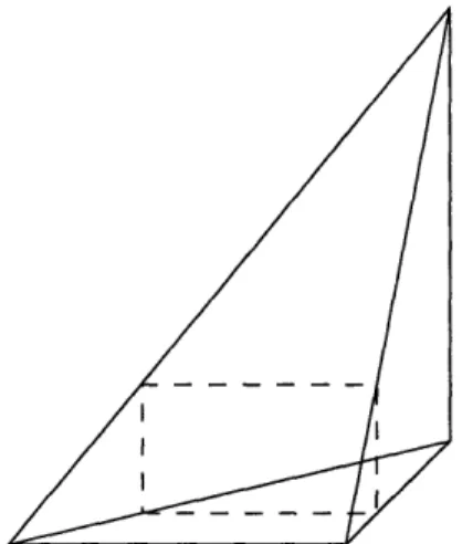
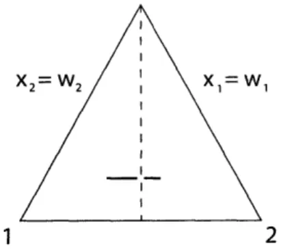
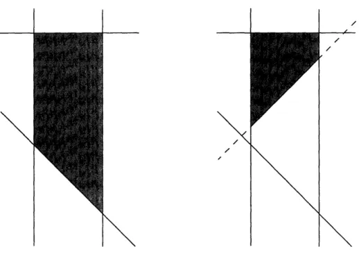
cuts that first isolate two pairs of vertices from each other, then separate each pair of vertices. He refers to such cuts as pair-isolating cuts. All such cuts he considered began with a pair-isolating slice: a hyperplane that is parallel to the two edges of the simplex connecting the pairs of vertices that they isolate. Such a hyperplane is shown in Figure 2-2. He then considered two different alternatives for how to separate the pairs of vertices. One was to separate them via a hyperplane parallel to a side of the simplex, and the other was to separate them via a hyperplane perpendicular to an edge of the simplex. He calls the pair-isolating cut induced by using a pair-isolating cut in conjunction with one of these two types of vertex-separating slices a pair-isolating side-parallel cut (abbreviated pair-side cut) and a pair-isolating edge-perpendicular cut (abbreviated pair-edge cut), respectively.

For his computational experiments, Mosk-Aoyama had to formulate appropriate versions of LP-UB, which entailed defining sub-distributions {Qi} and cells {Wj}, and computing density bounds ý4(Qi, WU). For this, he first fixes a discretization level d > 1. He then defines sub-distributions over pair-side cuts and pair-edge cuts which we will call pair-side cut 7anges and pair-edge cut ranges (analogous to Karger et al.'s spare ranges), and uses as his sub-distributions the set of all sparc ranges.

Figure 2-2: A pair-isolating slice. The intersection of the pair-isolating slice and the simplex is represented by the dashed region. This slice isolates the pair of vertices connected by the horizontal edge from the pair of vertices connected by the vertical edge.

pair-side cut ranges, and pair-edge cut ranges. For his cells, Mosk-Aoyama considers the possible orientations of all hyperplanar boundaries that can be generated by any cut chosen from his set of sub-distributions. He then performs d equally spaced hyperplanar slices of the simplex along each one of these orientations, and takes the resultant regions of the simplex as his cells. Note that this can be seen as a natural generalization of the way in which Karger et al. define their cells with respect to their choice of sub-distributions.

Mosk-Aoyama's results indicate that at a fixed discretization level, the introduc-tion of pair-side cuts and pair-edge cuts slightly improves the objective value of LP-UB. This led him to postulate that an optimal cutting scheme for k = 4 cannot be described as a probability distribution over sparcs. We will investigate this postulate in further detail in Chapter 5.

Chapter 3

Revisiting the Linear Program of

Karger et al.

In Section 2.2.3, we described an infinite-dimensional optimization problem, PRI-oo, that captures the problem of computing the minimum maximum density -r. Karger et al. formulated the finite linear program LP-UB, whose objective value is provably an upper bound on Tr. In this chapter, we discuss how we were able to loosen some of the constraints of that linear program in order to obtain stronger upper bounds. These upper bounds are given in Table 3.1, near the end of this chapter.

3.1

The constraints of Karger et al.

Recall the discretized version of PRI-oo used by Karger et al. for their computational experiments:

min 7

Q

_(LP-UB)

Q

pj-jQ(Q W) W - VWc W

Here, WV is a collection of cells, and the sums are taken over Q, a collection of d(istributions. The values {pQ} specify a probability distribution over the

sub-distributions. Each

4,(Q,

O(Q,

W) = sup TA(Q, s).

sES(w)

Recall that S(W) denotes the set of all segments whose endpoints lie in W. Let S1,2(W) denote the set of all 1, 2-aligned segments of S(W), and define the quantity

0

,2(Q, W) by

01,2(Q, W) = sup Tk(Q, s).

SES₁,2(W)

Karger et al. noted that O(Q, W) - 01,2(Q, W). This fact follows from Lemma 4 and the fact that each sub-distribution

Q

Karger et al. computed the upper bounds O(Q, W) as follows. Note that each sparc range Q can be itself thought of as a uniform probability distribution over k! sub-distributions, one per permutation of { 1,..., k}. If we let Q, be the sub-distribution corresponding to the permutation a, we have that

0

,

(Q, W)

•

sup

(

(Q, s).

(3.1)

Now, note that

sup >'rk(Qu,s) < sup Tk(Q,,s) (3.2)

SES1,2(WV) r sES1,2(VW)

E 01,2(Qa, 1¥).

To compute a bound '(Q, W), then, we can compute the values 01,2(Q0,, WI), and set

(Q,W)

)

=

-E

o2(Qr,

W).

(3.3)

To see that O(Q, W) is an upper bound on 01,2(Q, ii), note that 01,2(Q,

W)

1

=

(Q,

W).

Here, we have made use of equations (3.1) and (3.2).

The values 01,2(Qa, W) can be computed as follows. The vertices are processed in the order specified by cr, and the f-th slice distance pe is applied to the e-th vertex in the permutation, o(e).

When applying the f-th slice distance, we have three distinct possibilities. If the f-th coordinate of the sparc range is different from that of the cell, then the f-th slice will not pass through the cell: depending on whether the coordinate is larger or smaller the slice will either capture the entire cell or none of the cell. If the f-th coordinates are the same, then the slice might pass through the cell. In this case, we

can use the fact that the slice is uniformly distributed over a range.

A 1, 2-aligned segment can only be cut if the slices for vertex 1 or 2 go through the cell. If only one of the two slices goes through the cell, and no earlier slice goes through the cell, then the density of

Q,

<

In fact, we can see that 01,2(Qa, W) is exactly equal to 2d in the case when both slices go through the cell, and no earlier slice goes through the cell. It is not necessary to prove this in order to perform our goal of simply establishing an upper bound on 01.2(Q, W), but we include a proof for completeness:

Lemma 7. When the slices for both vertex 1 and 2 go through the cell, and no earlier slice goes through the cell,

Proof. Assume without loss of generality that the slice for vertex 1 comes before the slice for vertex 2. Consider then an infinitesimally small segment s that is arbitrarily close to the hyperplanes xl = wl and x₂ = w2. Then, the probability that the first

slice captures s is negligible, implying that the density contributions of the two slices can be added independently, for a total density arbitrarily close to d + d = 2d. Thus, 01,2(Qa, W) > 2d - E for all E > 0, implying that 01,2(Q,, W) = 2d. O

We can summarize our analysis by giving an explicit formula for 01,2(Q,, W). To do this, we first give an explicit formula for X(Qo, W), the number of slices of Q,

that can cut a 1, 2-aligned segment contained in W. Let the coordinates of Q be

(q1

,...

{(x

< xi

1)/d}.

For any i E

{1,..., k},

fi(Q, W) =

3m

otherwise.

The value of fi is 0 if some slice earlier than the i-th slice captures the cell W. Define 6(m, n) to be 1 if m = n and 0 otherwise.

Then, we have that

x(QU,

W)

=

(f"f(Q,

W)6(q,-I(l), w

)

+

f2W(Q,

W)6(q,-1(

Our explicit formula for 01,2(Q~, W4) then reads:

Cobining

(Q3.3), we obtain the density bound used by Karger et).

this

with

equation

al.:

'0(Q,

E

3.2

Exact density bounds

The analysis of the previous section relies on the application of inequality (3.2). A certain amount of slack is lost in doing so, resulting in sub-optimal density bounds

4(Q,

value is chosen adaptively with respect to the permutation a. On the other hand, equality can clearly only take place in (3.2) if that segment is chosen irrespective of

the permutation a.

As a result, the computed objective value of LP-UB only represents an upper bound of the maximum density of the corresponding cutting scheme. In this section, we show how to calculate the values 0(Q, W) exactly. Furthermore, we prove that with these new density bounds, the computed objective value of LP-UB in fact represents the exact value of the maximum density of the corresponding cutting scheme.

We begin by defining an alternate type of sub-distribution, closely related to a sparc range. As with sparc ranges, we fix an integer discretization level d and use one sub-distribution for each element of {0, 1,..., d- l}k - 1

. The sub-distribution for (qi, q2, ... qk-l) is induced by choosing a single value p uniformly at random from [0,

1/d],

Let Q, denote the set of uniform sparc ranges, and let W denote the same set of cells used by Karger et al. For our setup of LP-UB, we use Q, as our sub-distributions and W as our cells. One can prove that, if

Q

0(Q, UW:)

a : [7,3,1,4,2,6,5] a' : [7,3,2,4,1,6,5]

Figure 3-1: A 1,2-conjugate pair of permutations, for the k = 7 case. Note that the two permutations are identical except for the positions of 1 and 2.

WE

cW.

As before, each uniform sparc range

Q

k! _{sub-distributions, one per 1, 2-conjugate pair.}

Let Q,,,, be the sub-distribution corresponding to the permutation pair (a, a'). As before, we have that

sup

Pk(Q,'a,

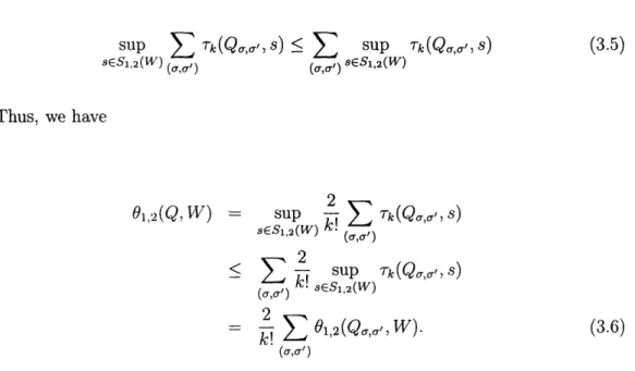
sES,2() ) () SES1,2(W) Thus, we have 01,2(Q,

W)

Here, the suprenma are taken over 1, 2-aligned segments, and the sumns are taken over all 1, 2-conjugate pairs.

density TA.(Q.o,) = supsg Tk(QT,&, s) when a and a' differ in their relative ordering of 1 and 2. The value they compute for this quantity is 1.5. Since a and a' differ in their relative ordering of 1 and 2 when (a, a') is a 1,2-conjugate pair, we are able to apply their analysis to compute the values of 01,2(Q,,,', W) for 1,2-conjugate pairs

(a, a').

Both a and a' are equally likely to be selected from Q,,,,, so that for any fixed segment s,

1

Tk(Q,,,', s) = 2 (-k(Q, s) + Tk(Q,', s)). (3.7) For 1, 2-conjugate pairs where only one of the slices for vertex 1 or vertex 2 can pass through the cell, the analysis of the previous section applies; we have that

Tk(Q,, s) = 7rk(Q~,, s) = d, and so

91,2(Q,,o', W) = sup k(Qa,,,, s) = d.

sES1,2(W)

The interesting case is when a and a' are permutations such that both the slices for vertex 1 and vertex 2 can pass through the cell.

Consider a 1, 2-aligned segment s. Define the following quantities:

mi -= min l -Wl xEs .M = max x - wi xEs m2 m= 12in2 -W2 XEs AM2 = max 2 -W2 xES

Note that Is = M8 - mi = M2 - m2. Without loss of generality, we may assume

that M1 < 'n2. This is because a 1, 2-aligned segment can be split in two with one

part closer to the hyperplane xl = wi and one part closer to the hyperplane x2 = w2, and our assumption then applies to each part separately (see Figure 3-2). Suppose that a is the permutation where 1 precedes 2, and that a' is the permutation where 2 precedes 1. Let us consider each of Tk(QU, s) and Tk-(Q,,, s) in turn.

1

Figure 3-2: A 1,2-aligned segment, split into two parts, with one part closer to the hyperplane xl = wl and one part closer to the hyperplane x2 w2. The dividing

hyperplane, represented by the vertical dashed line, can be expressed as x1 - X2 =

wl - w2. In this case, the assumption that M1

<

to the right of the dashed line.

p E [ml, M1] U [mn2, M2], which is a subset of [0, d] of measure 21s . On the other

hand, we can see that Tk(QM,, s) = d, since s will be cut iff p E [m2, M2], a subset of

[0, d] of measure IsI. The reason that s will not be cut if p E [ml, M1] is that the slice

for vertex 2 will capture all of s before the slice for vertex 1 has a chance to cut it. Figure 3-3 summarizes this argument.

Plugging into (3.7), then, we have that k(Q,,,', s) = 1.5d, and thus that

01,2(Q1,a', W) = sup Tk(Q,,a',

s)

sES1,₂(W)

If we define X as in the previous section, this analysis shows:

01.5d

if x(QU, W) = 2

d(-

_{(x(Q,, W) + x(Q,,, W)) else.}

Combining with (3.6) gives

O(Q, W) <

()),

1 2 M₁ M, I . I o m, m2 1/d o: / / / \ \ / V 1 2 1 2 7-1 2 1 2

Figure 3-3: A summary of the density contributions from a (1,2)-conjugate pair sub-distribution. At the top, we have a cell with a 1,2-aligned segment obeying the constraint M1 • m2. Directly below is the 1/d-length interval [0, 1/d], with the

dis-joint sub-intervals [mi, MI] and [fm2, M2] highlighted. The next row shows partitions

generated by o, and the bottom row shows partitions generated by a'. In both rows, the left side shows the case when p E [ml,

M

when p E [rm2, l2]. The key observation is that the segment is not cut when the

In fact, our analysis demonstrates that for segments s E S1,2(W), with the

prop-erty that M1 m Tk (Q,~,, s) exactly equals 01,2(Q~,I,, W) for all Q E Q, and all2,

1, 2-conjugate pairs (a, a'). Thus, the inequality of (3.5) is tight, implying that

O(Q,

W) =

g((Q,,

W)).

Note that without g, the right hand side simply becomes the density bound of Karger et al. given in (3.4).

Moreover, this implies that the inequality in (2.1), back in Section 2.2.3, is tight for the same reason. Thus, by substituting these values of 0(Q, W) for

4(Q,

3.3

Observations and results

We wrote a simple program to generate the linear programs described in this chap-ter automatically, and used CPLEX to solve them. While it is difficult to "prove" programs correct, our computations reproduced the results of Karger et al. prior to incorporating the function g in Equation (3.8), giving us confidence in the program's

correctness.

Table 3.1 summarizes the results of our computational experiments. Under the as-sumption that the programs were correct, the listed bounds are proven upper bounds on the integrality gap. The cutting schemes outputted by the program have maxi-mum density exactly equal to the given bounds. One unusual phenomenon we noticed was the corner cut probability did not decrease monotonically with respect to k as it had when using the Karger et al. bounds. In particular, the corner cut probability for k = 7 was higher than for other values of k. We have no hypothesis for why this might be the case. Perhaps the notion of corner cuts is not as significant as was originally suspected. In other respects. we did not notice any qualitative difference

discretization Karger et al. bounds Improved bounds

k level corner cut prob. bound corner cut prob. bound

4 36 .289 1.1539 .299 1.1494

5 18 .314 1.2161 .326 1.2071

6 12 .376 1.2714 .360 1.2573

7 9 .397 1.3200 .284 1.2967

Table 3.1: The upper bounds on the integrality gap obtained by improving the anal-ysis of Karger et al.

Chapter 4

Lower Bounding the Integrality

Gap

In this chapter, we present some approaches used to lower bound the value of T7. Our

approach has successfully generated computer-aided proofs of lower bounds on Tk-, as shown in Table 4.1 near the end of the chapter.

4.1

Preliminaries

Recall that wo(G) denotes the cost of the minimum k-way cut of G. For any em-bedding, a, of G into Ak, let

'y(G,

y(G, a) < y(G) for all embeddings a.

Theorem 2 tells us that 7-* is a value such that -y(G) K -F for all G. In order to prove a lower bound of To on TkZ, then, it suffices to demonstrate a particular graph Go a.nd a pa.rticular embedding ao such that y(Go, cao) > 7o. In fact, Theorem 2 guarantees the existence of such an embedded graph for any fixed 70 < T,, motivating us to search for bad embedded graphs.

4.2

Finding exact minimum k-way cuts

We wish to find embedded graphs a(G) for which the quantity 7(G, a) = woi(G)

is large. In order to compute this value, we need to compute the quantity wo(G). Unfortunately, finding the minimum k-way cut is a MAX-SNP hard problem (which is the reason we are performing this study in the first place). Thus, we set out to devise exact algorithms to solve minimum multiway cut efficiently in practice. Our approach uses the typical branch-and-bound paradigm.

In the remainder of this section, we will revert to using vertices to describe the elements of V. Nodes will refer to the elements of the enumeration tree.

4.2.1

Branch and bound enumeration tree

Note that any minimal k-way cut of a connected graph leaves every vertex connected to a unique terminal; i.e., it never disconnects a vertex from all the terminals. Thus, any minimal k-way cut of a connected graph can be thought of as an assignment of vertices to terminals, f : V - T, such that f(t) = t Vt E T. Conversely, any such assignment corresponds to a k-way cut of the graph: take as the cut the set of all edges (u, v) for which f(u)

#

#

This leads to the following equivalent phrasing of the minimum multiway cut problem: given a weighted graph G = (V, E), together with a set T C V, find an assignment f : V -+ T, with f(t) = t for all t E T, that minimizes the quantity

EEeLW(e), where L = {(u,v) E E :

f(u)

#

f(v)}.

tk

elements of T. This is in fact an instance of the more general discrete metric labeling problem, abbreviated DMLP. A DMLP branch-and-bound heuristic is described in [10], and our approach is based on it.

In the branch-and-bound enumeration tree, node i of the enumeration tree repre-sents a partial assignment, fi : Si --* T, of the vertices of some subset Si C V such that T C Si, and such that fi(t) = t Vt E T. The root node, r, is associated with the partial assignment where S,. = T. The children of any node i of the enumeration tree