Automating the Scientific Method
by
Span Spanbauer
Submitted to the Department of Mechanical Engineering
in partial fulfillment of the requirements for the degree of
Doctor of Philosophy in Mechanical Engineering
at the
MASSACHUSETTS INSTITUTE OF TECHNOLOGY
February 2021
© Massachusetts Institute of Technology 2021. All rights reserved.
Author . . . .
Department of Mechanical Engineering
Oct 26, 2020
Certified by . . . .
Ian W. Hunter
George N. Hatsopoulos Professor in Thermodynamics
Thesis Supervisor
Accepted by . . . .
Nicolas G. Hadjiconstantinou
Chairman, Department Committee on Graduate Theses
Automating the Scientific Method
by
Span Spanbauer
Submitted to the Department of Mechanical Engineering on Oct 26, 2020, in partial fulfillment of the
requirements for the degree of
Doctor of Philosophy in Mechanical Engineering
Abstract
We present a collection of novel computational tools designed to contribute to the goal of large-scale scientific automation. Deep Involutive Neural MCMC and other inference compilation techniques present a promising path to accelerating inference in probabilistic programs. Neural Group Actions provide foundational methods for learning symmetric transformations useful for the development of statistical models and probabilistic algorithms. Coarse-Grained Nonlinear System Identification provides an exceptional new model class for nonlinear dynamic systems, enabling accurate model identification with minimal experimental data. Optimization plus Stochastic
Interchange is a flexible new way to generate experimental stimuli, leading to optimally
informative measurements during system identification. Extended Koopman Models advance a new method for the optimal control of nonlinear systems. When coupled with high-throughput laboratory automation, these and other computational tools made possible by recent developments in artificial intelligence promise to revolutionize the way we do science and engineering.
Thesis Supervisor:
Ian W. Hunter, George N. Hatsopoulos Professor in Thermodynamics
Thesis Committee:
Kamal Youcef-Toumi, Professor of Mechanical Engineering Tonio Buonassisi, Professor of Mechanical Engineering
First and foremost, I would like to express my deepest gratitude to my thesis advisor and mentor, Ian Hunter. We met a full decade ago when I took his undergraduate course ‘Measurement and Instrumentation.’ I had been training to be a theorist in mathematics and physics, and I had just begun to realize that I wanted to have a more tangible impact through engineering and entrepreneurship. Ian, an accomplished Renaissance-type polymath, helped me find a path that unified my theory background with new skills in engineering and business. His steadfast support and encouragement to freely explore across traditional domain-boundaries enabled me to grow and find my calling in the automation of scientific exploration and technology development. Ian’s group, the MIT BioInstrumentation Laboratory, reflects his mentorship style. It is a uniquely multidisciplinary group bridging biology, optics, mathematics, mechanics, materials, electronics, chemistry, and computation. Every member of the laboratory naturally becomes an expert in several of these fields by collaborating on high-impact, discipline-spanning projects. I would like to thank every brilliant member of the lab, and I will call out Cathy Hogan and Mike Zervas specifically, two individuals who have been with me through the years.
I want to thank another community, MIT’s Epsilon Theta (ET) independent living group. The friends I’ve made at ET have been an endless source of creative energy. From learning how to create ‘deep fake’ videos together, to inventing new chess variants, to improvised cooking, it is always an adventure.
I would also like to thank my co-authors. Luke Sciarappa is a good friend and brilliant mathematician I met at ET. Cameron Freer and Vikash Mansignka of the MIT Probabilistic Computing Group were critical in helping me grow as a scientific author. And of course I cannot thank my mentor Ian enough.
I want to thank my family for striving to create opportunities for me to learn and grow. They’ve had a deep influence on me, without which I wouldn’t be who or where I am today.
I would also like to thank my other close friends, including the TB living group, Jayson Lynch, Katie Sedlar, Mollie Wilkinson, and Carter Huffman. I especially would like to thank my close friend of many years, Sarah Bricault, who has been an invaluable source of support and feedback during my graduate studies. Throughout the years we’ve shared many memories, including raising our cats Artemis, Kegan, and Nita, rescuing a baby squirrel, and having many holidays together.
1 Introduction 15
2 Deep Involutive Generative Models for Neural MCMC 23
2.1 Introduction . . . 25
2.2 Background . . . 26
2.3 Involutive Neural Networks . . . 29
2.3.1 Involutive function blocks . . . 30
2.3.2 Involutive permutation blocks . . . 31
2.3.3 Involutive matrix blocks . . . 32
2.3.4 Deep involutive networks . . . 33
2.4 Universality of Involutive Generative Models . . . 35
2.4.1 Proof of Universality . . . 36
2.4.2 Proof of Validity . . . 44
2.5 Training and sampling algorithm . . . 48
2.6 Experimental Results . . . 53
2.7 Discussion . . . 55
3 Neural Group Actions 57 3.1 Introduction . . . 58
3.2 Background . . . 60
3.3 Neural Group Actions . . . 61
3.3.3 Generative models derived from a Neural Group Action . . . . 67
3.4 Experiment . . . 68
3.4.1 Architecture and training . . . 68
3.4.2 Results. . . 69
3.5 Discussion . . . 70
4 Coarse-Grained Nonlinear System Identification 73 4.1 Introduction . . . 75
4.2 Background . . . 76
4.2.1 Volterra series expansions . . . 76
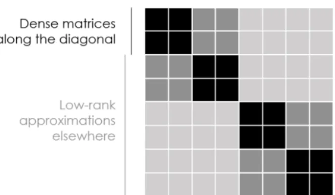
4.2.2 Hierarchical matrices and tensors . . . 78
4.3 Synthetic experiment . . . 80 4.4 Physical experiment . . . 83 4.4.1 Experimental apparatus . . . 83 4.4.2 Input signal . . . 85 4.4.3 Model details . . . 85 4.4.4 Results. . . 86 4.5 Discussion . . . 89
5 Rapid Generation of Stochastic Signals with Specified Statistics 91 5.1 Introduction . . . 93
5.2 Background . . . 94
5.3 Algorithm . . . 96
5.4 Results . . . 98
5.5 Discussion . . . 102
6 Extended Koopman Models 103 6.1 Introduction . . . 104
6.3 Extended Koopman Models . . . 108
6.4 Architecture . . . 109
6.5 Training . . . 110
6.6 Experimental Details and Results . . . 111
6.6.1 Particle in a double-well potential . . . 112
6.6.2 Quadrupedal robot . . . 114
6.7 Discussion . . . 116
7 Future Directions 119
2.1 Definition (Involutive function block) . . . 30
2.2 Definition (Involutive permutation block) . . . 31
2.3 Definition (Involutive matrix block) . . . 32
2.4 Lemma (Every involutive matrix block is involutive) . . . 32
2.5 Definition (Involutive network) . . . 34
2.6 Theorem (Involutive generative models are universal.) . . . 36
2.7 Theorem (Hornik [40, Thm. 3]) . . . 37
2.8 Lemma (Conditioned on the event 𝐴𝜖𝑚, we have the following:) . . 39
2.9 Lemma (Conditioned on the event 𝐴𝜖𝑚, the random variable ℐ𝜖𝑚[𝜑] converges in distribution to 𝑇 [𝜑] as 𝜖𝑚 → 0.) . . . 39
2.10 Lemma (As 𝛿𝑚 → 0, the function ̂︀ℎ𝜖 𝑚,𝛿𝑚 converges uniformly to ℎ𝜖𝑚 on Ω × 𝐵3(0𝑛+6) and its inverse ̂︀ℎ−1 𝜖𝑚,𝛿𝑚 converges to ℎ −1 𝜖𝑚 on Ω +× Ω+.) 41 2.11 Lemma (Consider the random variable 𝑥 := 𝜑⌢𝜋. Conditioned on the event 𝐴𝜖𝑚, the function ℐ̂︀𝜖𝑚,𝛿𝑚(𝑥) converges pointwise to ℐ𝜖𝑚(𝑥), as 𝛿𝑚 → 0.) . . . 41
2.12 Lemma (Conditioned on the event 𝐴𝜖𝑚, the random variableℐ̂︀𝜖𝑚,𝛿𝑚[𝜑] converges in distribution to ℐ𝜖𝑚[𝜑] as 𝛿𝑚 → 0.) . . . 42
2.14 Lemma (𝑃𝐻 is symmetric:) . . . 46
2.15 Lemma (𝑃𝐴 satisfies the following simpler form:) . . . 47
2.16 Lemma (𝑃𝑆𝑃𝐺𝑃𝐴 is symmetric:) . . . 47
2.17 Theorem (The Markov chain defined by transitions 𝑃𝑀 has 𝑃𝑆 as a
stationary distribution.) . . . 47
3.1 Lemma (Construction for a Neural Group Action:) . . . 62
3.2 Lemma (If 𝐻 and all of the 𝑇𝑠 are volume preserving, then so is the
2.1 Comparison of performance on a mixture of two Gaussians . . . 27
2.2 System diagram showing that two composed involutive function blocks forms the identity operation. . . 30
2.3 System diagram of a deep involutive neural network . . . 35
2.4 Comparison of convergence rate of Involutive Neural MCMC and A-NICE-MC on a mixture of six 2D Gaussians . . . 54
2.5 Quantitative comparison of convergence rates of Involutive Neural MCMC and A-NICE-MC . . . 54
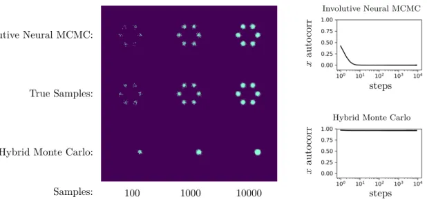
2.6 Comparison of mixing of Involutive Neural MCMC and Hybrid Monte Carlo on a mixture of 6 2D Gaussians. . . 55
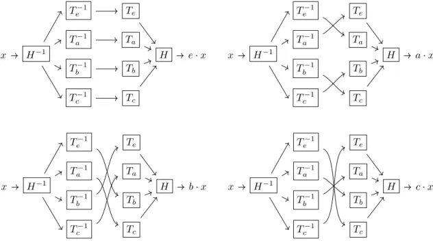
3.1 Architecture for a 𝐾4–Neural Group Action . . . 65
3.2 Single qubit transformations learned by a 𝑄8–Neural Group Action . 70
4.1 Structure of a hierarchical matrix . . . 78
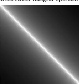
4.2 Discretized integral operator . . . 81
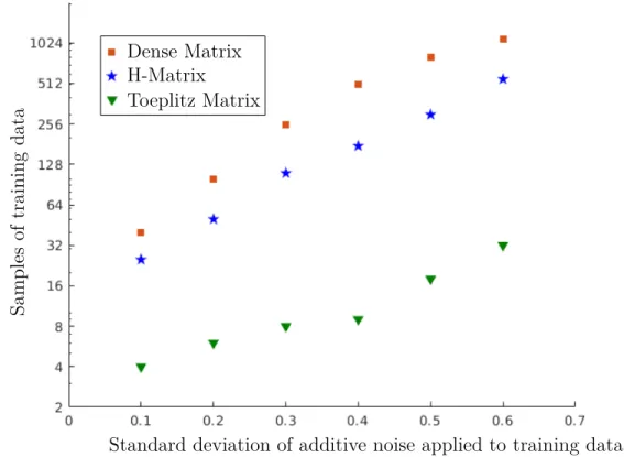
4.3 Synthetic training data required to achieve a given accuracy in held-out data . . . 82
4.4 Experimental apparatus . . . 84
4.7 Identified second order Volterra kernel . . . 89
5.1 Comparison of convergence rate (10k and 100k sample signals) . . . . 99
5.2 Comparison of signals generated via optimization plus stochastic inter-change vs optimization on its own . . . 100
5.3 Autocorrelation function of the generated signal . . . 101
5.4 Cumulative distribution function of the generated signal . . . 101
6.1 Example architecture for Extended Koopman modeling . . . 110
6.2 Trajectory prediction for a particle in a double-well potential . . . 113
6.3 Model of the quadrupedal robot as rendered in the physics engine . . 114
Introduction
Scientific advances often come in the form of a new language for describing a do-main [57]. These languages couple a syntax, taking the form of a mathematical theory, with semantics describing how that theory relates to observations in the physical world. Canonical examples of new languages include the theory of general relativity for describing the structure of spacetime, the action principle and the path integral formulation of quantum field theory, the Turing machine for modeling computation, the molecular orbital theory of chemistry, and the Hodgkin-Huxley model of neural action potential propagation. Each of these languages take existing observations and re-explain them in a much simpler form; this new form then constrains and shapes the form of new hypotheses, essentially acting as a strong statistical prior to guide future science.
These languages need not be sweeping reformulations of an entire discipline; they may be narrow in scope, they may be incremental in impact, and they may reuse existing mathematical machinery. For example, a proposal to use the Volterra series expansion [31] to model the nonlinear dynamics of NiTi shape memory alloy [79] would constitute a scientific advance so long as the model had explanatory power.
Under this view, a primary role of scientists is to formulate new languages which accurately and parsimoniously describe observations. Once a scientist has formally described classes of models, priors on those models, and the semantics of how experi-ments connect to those models, then other scientific activities, including the design of optimal experiments and the collection and analysis of data, are in striking distance of full automation.
Achieving this level of automation requires the development of automated laboratory equipment, ideally capable of flexible high-throughput experimentation in the domain under study. It is our view that the development of this flexible physical automation is as important as the development of computational tools enabling flexible statistical automation; however this thesis focuses primarily on the latter.
Probabilistic programming [33] is a leading candidate for a general method for scientists to express model classes within their domain. Modern probabilistic programming languages such as Gen [25], Stan [18], and PyMC3 [95] provide a straightforward and general way to express computable, differentiable classes of models with quantified uncertainty.
Once a scientist has expressed a class of models along with the semantics of possible experiments, it is possible to perform automated model identification. Bayesian optimization [78] can be used to design optimal experiments. Once data is available, automated inference algorithms included as part of a probabilistic programming language can be used to infer the model structure and parameters best describing the system under study.
However, the general purpose inference algorithms available in probabilistic pro-gramming languages, typically some form of Markov Chain Monte Carlo (MCMC) inference [83], are often too slow to be of practical use when performing inference on large, complex, or computationally expensive classes of models. Some probabilistic programming languages such as Gen [25] have interfaces for users to design their own
accelerated inference algorithms specialized to their particular problem. Unfortunately, the design of these specialized inference algorithms requires fairly detailed knowledge of computational statistics, which is not as broadly accessible as development of the model classes alone.
Fortunately, there is a promising path towards broadly-accessible, fast, general-purpose inference for probabilistic programs: the development of inference compilation tech-niques [62]. An inference compilation technique takes a model class, for example as expressed in a probabilistic programming language, and automatically ‘compiles’ it into an accelerated inference algorithm, optimized and specialized for the model class. An inference compilation technique which uses deep learning to accelerate importance sampling [8] was applied in 2019 to accelerate inference for a problem in particle physics, specifically of the branching ratios associated with 𝜏 lepton decay [9]. In Chapter2[106] we describe a novel inference compilation algorithm, Deep Involutive
Neural MCMC, which uses deep learning to accelerate Markov Chain Monte Carlo
inference. We demonstrate that it converges faster than an existing neural MCMC algorithm, A-NICE-MC [101], and that it mixes faster than a commonly used gradient-accelerated MCMC algorithm, Hybrid Monte Carlo [29]. We’re optimistic that this and further developments in inference compilation will drive adoption of probabilistic programming as a meta-language for formalizing scientific theories, appropriate for driving automated experiment design and data analysis.
Development of Deep Involutive Neural MCMC involved designing novel deep neural network architectures satisfying special mathematical properties. These mathematical properties were useful in making our inference compilation algorithm both fast and provably correct. First, we introduced neural networks 𝒩 which are exactly involutive, that is, which satisfy 𝒩 (𝒩 (𝑥)) = 𝑥 for any data 𝑥, no matter the choice of parameters of the neural network. Second, we showed how to constrain these networks to exactly preserve volume, that is, to have a Jacobian whose determinant has magnitude 1.
In addition to proving our method correct, we also proved a universality property showing that our inference compilation algorithm is the first neural MCMC algorithm which if given an inference problem and a level of accuracy will, given enough network capacity and training time, learn how to solve that inference problem to that accuracy in a single step.
In Chapter 3 [105] we introduce Neural Group Actions, which are a a dramatic generalization of the involutive neural networks used for Deep Involutive Neural
MCMC. For any finite symmetry, we show how to design a collection of neural
networks which exactly satisfy the laws of that symmetry. Involutive neural networks are the special case satisfying the law 𝒩 (𝒩 (𝑥)) = 𝑥 of the symmetry expressed by Z2,
the cyclic group of order 2. We also show how to constrain Neural Group Actions to exactly preserve volume, just as we did for involutive neural networks. We provide an experiment showing that a Neural Group Action satisfying the laws of a larger group, the quaternion group 𝑄8, can be used to model how a certain set of quantum
gates satisfying the 𝑄8 group laws act on single-qubit quantum states. Neural Group
Actions will be useful in modeling symmetric physical transformations, most commonly
appearing in quantum physics and statistical physics, as well as neurally accelerating probabilistic algorithms such as Deep Involutive Neural MCMC.
Until this point we have spoken in fully domain agnostic terms, and described infer-ence techniques applicable to any domain. We now restrict ourselves to dynamical systems [88], that is, systems which evolve in time. The statistical study of this broad class of systems is called system identification [67].
One notable model class for dynamical systems is the Volterra series expansion [31], which directly generalizes the theory of linear dynamic systems to arbitrary nonlinear dynamic systems. It has seen extensive application in fields including biology [55,
96, 19], chemistry [6], electronics [114, 82, 47], optics [11, 48], and energy storage and transfer [35, 43, 60]. The Volterra series expansion is a particularly flexible
model class, which perhaps accounts for its success. However, it is in some regards too flexible; Volterra series models require a large number of parameters to specify, particularly when modeling highly nonlinear systems. This lack of parsimony means that identifying an accurate Volterra model can require an impractically large amount of experimental data.
In Chapter4 [102] we introduce Coarse-Grained Nonlinear Dynamics, a new language for describing dynamical systems based on a dramatic simplification of the Volterra series expansion which avoids losing useful representational power. We accomplish this by imposing a form of temporal coarse graining closely related to the fast multipole method [92], famous for its ability to simulate 𝑛-body dynamics in only 𝒪(𝑛) time. This temporal coarse-graining structurally imposes a strong statistical prior which we leverage in a novel system identification technique, Coarse-Grained Nonlinear System
Identification, enabling the identification of accurate models of nonlinear dynamic
systems with minimal experimental data. The reduction in the amount of experimental data required, as compared to standard identification of a Volterra series, is so extreme that its scaling lies in a strictly smaller multiparameter complexity class FPT rather than XP [28]; this is a superpolynomial reduction in the amount of experimental data required for highly nonlinear systems.
To rapidly learn an accurate model of a system one must, in addition to choosing a good model class, perturb the system so as to generate highly informative experimental data. With some prior knowledge of the system, one may use Bayesian optimization [78] to design optimal experimental stimuli leading to informative measurements. This objective can often be framed as generating a stochastic input signal with specific statistics, such as its autocorrelation function and probability density function.
In Chapter 5 [104] we describe a new algorithm, designed for generating optimal experimental stimuli, which produces stationary stochastic signals with specified statistics. We focus on generating stochastic signals with specified autocorrelation
and probability density functions, though a primary feature of our method is the ease by which it can be generalized to produce signals with other combinations of statistics. We combine gradient optimization with a prior technique based on stochastic interchange of samples [41], leading to strictly better time complexity than stochastic interchange alone and much better stationarity than optimization alone. This enables the generation of long stochastic signals with flexible combinations of statistics, ideal for use in optimal system identification.
A common reason to identify a model of a dynamical system is to subsequently control it. Of the many approaches to control, one common strategy is to combine an approximate Bayesian filter [97] with a model predictive controller [17]. For linear dynamic systems this approach is called a linear quadratic Gaussian regulator, for which the control problem can be solved quickly via quadratic programming [81]. While the problem of linear control is settled, the control of nonlinear systems is an extremely active area [100, 61, 107] currently heavily influenced by deep learning. One unusual new approach to the optimal control of nonlinear systems leverages a method of globally linearizing nonlinear systems first described in 1931: Koopman operators [52]. This approach entails finding a nonlinear transformation which ‘lifts’ the system state to a new space in which its dynamics are linear. One can then perform fast, optimal linear model predictive control in the lifted space. Surprisingly, the Koopman operator approach is universal; every dynamical system, no matter how nonlinear, can be approximated arbitrarily well via a Koopman model and, in principle, controlled in this way. At first appearance this approach to control seems extremely promising. Unfortunately, Koopman models of typical systems must be impractically large in order to have good accuracy. Koopman models of a practical size can only predict accurately out to a short time horizon, beyond which they cannot be used for control.
models, dramatically increasing their accuracy without sacrificing the potential for fast, globally optimal control. We generalize Koopman models in two ways. First, we replace the standard linear dynamics in the lifted space with more general convex dynamics. Second, we allow the lifted dynamics to depend on an invertible transformation of the control signal. To perform fast, globally optimal control, one would use convex optimization in the lifted space on the transformed control coordinates, and then use the inverse of the transformation to obtain the true optimal control signal. We show experimentally for two nonlinear, nonconvex systems that an Extended Koopman Model using a lifted space of the same dimension as a standard Koopman model can predict accurately out to a time horizon an order of magnitude longer. This development may lead to new practical methods of globally optimal control for nonlinear, nonconvex systems.
These various computational tools were designed to contribute to the goal of large-scale scientific automation. Each of these contributions may only play a small part, however I am optimistic that further work—academic, entrepreneurial, and so on—will lead to a phase change in the way we do science, greatly improving the scientific and technological capabilities of our species.
Deep Involutive Generative Models
for Neural MCMC
The contents of this chapter were taken from the following publication:
S. Spanbauer, C. Freer, and V. Mansinghka. Deep Involutive Generative Models for Neural MCMC. arXiv preprint arXiv:2006.15167, 2020
for Neural MCMC
Span Spanbauer Cameron Freer Vikash Mansinghka
MIT MIT MIT
Abstract
We introduce deep involutive generative models, a new architecture for deep generative modeling, and use them to define Involutive Neural MCMC, a new approach to fast neural MCMC. An involutive generative model represents a probability kernel
𝐺(𝜑 ↦→ 𝜑′) as an involutive (i.e., self-inverting) deterministic function 𝑓 (𝜑, 𝜋) on an enlarged state space containing auxiliary variables 𝜋. We show how to make these models volume preserving, and how to use deep volume-preserving involutive generative models to make valid Metropolis–Hastings updates based on an auxiliary variable scheme with an easy-to-calculate acceptance ratio. We prove that deep involutive generative models and their volume-preserving special case are universal approximators for probability kernels. This result implies that with enough network capacity and training time, they can be used to learn arbitrarily complex MCMC updates. We define a loss function and optimization algorithm for training parameters given simulated data. We also provide initial experiments showing that Involutive
Neural MCMC can efficiently explore multi-modal distributions that are intractable for
Hybrid Monte Carlo, and can converge faster than A-NICE-MC, a recently introduced neural MCMC technique.
2.1
Introduction
Markov Chain Monte Carlo (MCMC) methods are a class of very general techniques for statistical inference [13]. MCMC has seen widespread use in many domains, including cosmology [30], localization [85], phylogenetics [93], and computer vision [58]. For the Metropolis–Hastings class of MCMC algorithms, one must specify a proposal distribution 𝑞(𝜑 ↦→ 𝜑′). Convergence will be slow if the proposal distribution is poorly tuned to the posterior distribution 𝑝(𝜑′|𝐷). Conversely, if one could use a perfectly-tuned proposal distribution — ideally, the exact posterior 𝑞(𝜑 ↦→ 𝜑′) = 𝑝(𝜑′|𝐷) — then MCMC would converge in a single step.
Neural MCMC refers to an emerging class of deep learning approaches [101, 110, 64] that attempt to learn good MCMC proposals from data. Neural MCMC approaches can be guaranteed to converge, as the number of MCMC iterations increases, to the correct distribution — unlike neural variational inference [77, 50,91], which can suffer from biased approximations. Recently, Song et al. [101] suggested that involutive neural proposals are desirable but difficult to achieve:
“If our proposal is deterministic, then 𝑓𝜃(𝑓𝜃(𝑥, 𝑣)) = (𝑥, 𝑣) should hold for
all (𝑥, 𝑣), a condition which is difficult to achieve.” [101]
Contributions. This paper presents a solution to the problem of learning involutive
proposals posed by [101]. Specifically, it presents the following contributions:
1. This paper introduces involutive neural networks, a new class of neural networks that is guaranteed to be involutive by construction; we also show how to constrain the determinant of the Jacobian of these networks to have magnitude 1, that is, to preserve volume.
new class of auxiliary variable models, and shows that the volume-preserving ones can be used as Metropolis–Hastings proposals.
3. This paper proves that volume-preserving involutive generative models are universal approximators for transition kernels, justifying their use for black-box learning of good MCMC proposals.
4. This paper describes a new, lower-variance estimator for the Markov-GAN training objective [101] that we use to train involutive generative models. 5. This paper shows that Involutive Neural MCMC can improve on the convergence
rate of A-NICE-MC, a state-of-the-art neural MCMC technique. 6. This paper illustrates Involutive Neural MCMC on a simple problem.
We motivate our approach by showing that several common Metropolis–Hastings proposals are special cases of involutive proposals (Section2.2). We then show that by using a class of exactly involutive neural network architectures (Section 2.3) satisfying an appropriate universality condition (Section 2.4) and using adversarial training (Section 2.5), we can find involutive proposals that empirically converge extremely
rapidly (Section 2.6).
2.2
Background
Recall that the speed of convergence of a Metropolis–Hastings algorithm is highly dependent on how well the proposal distributions match the posterior.
In order to use a given proposal distribution, one typically constructs a transition which satisfies the detailed balance condition, which (in an ergodic setting) ensures convergence to the posterior. Satisfying this condition for a general proposal is hard, which has led researchers to use smaller classes of proposals for which this problem
𝜑 𝑃true(𝜑) True posterior 𝑃true(𝜑) = 12 [︁ 𝑃𝑁 (0.5,0.05)(𝜑) + 𝑃𝑁 (−0.5,0.05)(𝜑) ]︁ 𝜑′ 𝜑 𝜑 High-variance Gaussian 𝜑′ 𝜑 𝜑 Low-variance Gaussian 𝜑′ 𝜑
Hybrid Monte Carlo
𝜑′ 𝜑 Involutive Neural MCMC steps auto corr steps auto corr steps auto corr steps auto corr
Figure 2.1: Consider the problem of using MCMC to sample from a mixture of two Gaussians. Here, each trace shows the distribution (rescaled for clarity) of proposed state transitions 𝜑′ from a given initial state 𝜑. High-variance Gaussian proposals are a poor approximation of the posterior, and hence converge slowly. Low-variance Gaussian proposals fail to mix between the two modes because proposals between the modes will be rejected with high probability. Hybrid Monte Carlo converges quickly within a mode, but also fails to mix between modes. Proposals from Involutive Neural MCMC nearly match the posterior from every state, mixing and nearly converging in a single step.
is tractable. Our method, Involutive Neural MCMC, satisfies detailed balance for a universal class of proposal distributions, drawn from a generative model specified by a volume-preserving involutive function. Our method builds on previous work on invertible neural networks [3], for example the architecture we use in our constructive proof of universality makes use of additive coupling layers [26] which have been cascaded [27,44]. We now describe several existing classes of proposals, and observe that each can be viewed as an involutive proposal.
The canonical example of a class of proposal distributions is the collection of shifts by a multivariate Gaussian. These immediately satisfy detailed balance due to their
symmetry, that is, the probability 𝑃 (𝜑 ↦→ 𝜑′) of a forward transition is equal to the probability 𝑃 (𝜑′ ↦→ 𝜑) of a backward transition. However, multivariate Gaussians are usually poor approximations of the posterior, leading to slow convergence. We observe that these proposals can be viewed as involutive proposals: choose the auxiliary variable
𝜋 to be a sample from the multivariate Gaussian, and define the state transition to be
(𝜑, 𝜋) ↦→ (𝜑 + 𝜋, −𝜋).
Another example class of proposal distributions is those generated by Hamiltonian dynamics in the Hybrid Monte-Carlo algorithm [29]. These proposals can be shown to satisfy detailed balance because they are involutive: proposals for Hybrid Monte Carlo are obtained by simulating a particle for a certain amount of time and then negating its momentum; if one performs this operation twice, the particle will end in its initial state.
Recently, researchers have begun using neural networks to parameterize classes of proposal distributions, leading to neural MCMC algorithms. The A-NICE-MC method involves choosing a symmetric class of proposals parameterized by an invertible neural network: its Metropolis–Hastings proposal assigns 1/2 probability to the output of the network, and 1/2 to the output of the inverse of the network. This proposal is symmetric, and hence satisfies detailed balance. However, one can also view it as invo-lutive. Specifically, let 𝑓 be an invertible neural network, and 𝜋 ∼ 𝑁 (0, 1) the auxiliary variable. Define the state transition to be (𝜑, 𝜋) ↦→
⎧ ⎪ ⎪ ⎨ ⎪ ⎪ ⎩ (𝑓 (𝜑), −𝜋) if 𝜋 > 0, (𝑓−1(𝜑), −𝜋) otherwise.
We have seen that all of these examples are special cases of involutive proposals. We now introduce a class of exactly involutive neural network architectures (Section 2.3) and show that they satisfy a universality condition, and so may be used to approximate any involutive proposal arbitrarily well (Section 2.4).
2.3
Involutive Neural Networks
In this section, we describe how to build deep neural networks which are exactly involutive by construction. To do this, we first describe three kinds of smaller involutive building blocks, and then we describe how to compose these blocks to form a deep involutive network:
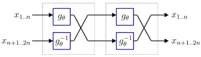
• Involutive function blocks, which are fairly general nonlinear maps, but do not fully mix information, in that every element of the output is independent of half of the elements of the input.
• Involutive permutation blocks, which are linear maps and cannot be opti-mized, but can mix information.
• Involutive matrix blocks, which are linear maps, but can be optimized and can mix information.
By composing these blocks in a particular way, we can create deep networks which have high capacity and are exactly involutive. We further show that each involutive block is either preserving or can be made so, leading to high-capacity volume-preserving involutive networks appropriate for use as MCMC transition kernels. In Section 2.4, we prove that these deep involutive networks are universal in a particular sense.
Let 𝑎⌢𝑏 denote the concatenation of vectors 𝑎 and 𝑏, and write 𝑎𝑗..𝑘 to denote the
restriction of the vector 𝑎 to its terms indexed by 𝑗, 𝑗 + 1, . . . , 𝑘. Let Id𝑛 denote the
Composition of two involutive function blocks 𝑥1..𝑛 𝑥1..𝑛 𝑥𝑛+1..2𝑛 𝑥𝑛+1..2𝑛 𝑔𝜃 𝑔𝜃−1 𝑔𝜃 𝑔𝜃−1
Figure 2.2: System diagram showing that two composed involutive function blocks forms the identity operation.
2.3.1
Involutive function blocks
Involutive function blocks enable the application of fairly general nonlinear functions to the input data. In the typical case, they are parameterized by an invertible neural network [3], which is itself parameterized by two neural networks of arbitrary architecture.
Definition 2.1 Involutive function block
Let 𝑛 ∈ N and let 𝑔 : R𝑛→ R𝑛 be a bijection.
Define the involutive function block 𝐼𝐹2𝑛,𝑔: R2𝑛→ R2𝑛 by
𝐼𝐹2𝑛,𝑔(𝑥) := 𝑔−1(𝑥𝑛+1..2𝑛)⌢𝑔(𝑥1..𝑛).
Observe that (𝐼𝐹2𝑛,𝑔 ∘ 𝐼𝐹2𝑛,𝑔)(𝑥) = (𝑔−1 ∘ 𝑔)(𝑥1..𝑛)⌢(𝑔 ∘ 𝑔−1)(𝑥𝑛+1..2𝑛) = 𝑥, where ∘
denotes function composition, and so the function 𝐼𝐹2𝑛,𝑔 is indeed an involution. See Fig. 2.2 for a system diagram depicting this fact. Further note that 𝑛 and 𝑔 are uniquely determined by the function 𝐼𝐹2𝑛,𝑔, and so when this function is induced by some neural net (i.e., when 𝑔 is itself induced by a neural net), we may think of 𝐼𝐹2𝑛,𝑔 as a neural net with the same parameters as the neural net inducing 𝑔. In this case we will sometimes elide the distinction between the function and this neural net, or refer to the function induced by the neural net by the same symbol.
If the parameter 𝑔 is volume-preserving, that is, the determinant of its Jacobian has magnitude 1, then we observe that the resulting involutive function block is also volume-preserving by considering the properties of the determinant of block matrices. In our experiments we obtain volume-preserving involutive function blocks by parameterizing 𝑔 using NICE additive coupling layers [26] which have been cascaded [27, 44], since these NICE layers preserve volume.
2.3.2
Involutive permutation blocks
One can see from Fig. 2.2, as previously noted, that each output of an involutive function block is independent of half of the inputs. In order to create more general involutive networks without this property, we mix information by applying an involutive permutation.
Definition 2.2 Involutive permutation block
Let 𝑛 ∈ N and let 𝜎 be an involution on the set {1, . . . , 𝑛}. Let 𝜎 denote the matrix defined by 𝜎𝑖𝑗𝑒𝑗 = 𝑒𝜎(𝑖) for 𝑖, 𝑗 ∈ {1, . . . , 𝑛}, where the 𝑒𝑖 are basis vectors.
Define the involutive permutation block 𝐼𝑃𝑛,𝜎: R𝑛 → R𝑛 by
𝐼𝑃𝑛,𝜎(𝑥) := 𝜎𝑥.
Note that 𝑛 and 𝜎 are uniquely determined by the function 𝐼𝑃𝑛,𝜎. We may also think of this function as a linear layer with no parameters in a neural net.
Observe that involutive permutation blocks, as permutations, are volume preserving.
One may use any involutive permutation 𝜎: we use a specific choice of 𝜎 in the proof of universality, and we use uniformly random involutive permutations in the experiments. An algorithm for sampling uniformly from the space of 𝑛-dimensional
involutive permutations is described in [5].
2.3.3
Involutive matrix blocks
As an alternative to involutive permutations, we may use a different class of involutive matrices to mix information. Compared to involutive permutations, involutive matrix blocks have the advantage that they can be optimized. This is because they are parameterized by two arbitrary nonzero vectors of real numbers.
Definition 2.3 Involutive matrix block
Let 𝑛 ∈ N and let 𝑣, 𝑤 ∈ R𝑛∖ {0𝑛}.
Define the involutive matrix block 𝐼𝑀𝑛,𝑣,𝑤: R𝑛→ R𝑛 by
𝐼𝑀𝑛,𝑣,𝑤 := Id𝑛−
2𝑣 ⊗ 𝑤
𝑣 · 𝑤 .
Involutive matrix blocks are in fact involutive; for completeness, we include the following proof, adapted from [63].
Lemma 2.4 Every involutive matrix block is involutive Every involutive matrix block is involutive.
Proof. Let 𝑛 ∈ N and 𝑣, 𝑤 ∈ R𝑛∖ {0𝑛}. The product of 𝐼𝑛,𝑣,𝑤
𝑀 with itself is the identity:
(︃ Id𝑛− 2 𝑣 ⊗ 𝑤 𝑣 · 𝑤 )︃(︃ Id𝑛− 2 𝑣 ⊗ 𝑤 𝑣 · 𝑤 )︃ = Id𝑛− 4 𝑣 ⊗ 𝑤 𝑣 · 𝑤 + 4 (𝑣 ⊗ 𝑤)(𝑣 ⊗ 𝑤) (𝑣 · 𝑤)2 = Id𝑛 Hence 𝐼𝑀𝑛,𝑣,𝑤 is involutive.
Not all involutive matrices are involutive matrix blocks; for example, the identity matrix is involutive but not an involutive matrix block.
Compared to involutive permutation blocks, involutive matrix blocks potentially allow for freer mixing between dimensions, and can also be optimized.
Note that 𝑛, 𝑣, and 𝑤 are uniquely determined by the function 𝐼𝑀𝑛,𝑣,𝑤 if we constrain |𝑤| = 1, and so without loss of generality we may think of it as a neural net with parameters 𝑣 and 𝑤.
Observe that involutive matrix blocks are volume preserving by the matrix determinant lemma.
2.3.4
Deep involutive networks
In order to create deep networks which have high capacity and which are exactly involutive, we want to compose several involutive blocks. For the resulting network to be involutive, we must compose them in particular ways.
Definition 2.5 Involutive network
Let 𝑛 ∈ N. We say that a neural network is an invertible network of dimension
𝑛 if it induces a bijection from R𝑛 to R𝑛 and its inverse is also expressible as a neural
network. Write V𝑛 to denote the set of invertible neural networks of dimension 𝑛.
A neural network is an involutive network of dimension 𝑛 if the function it induces is contained in the closure of the following operations. Write I𝑛 for the set of all such
functions.
• 𝐼𝐹𝑛,𝑔 ∈ I𝑛 for 𝑔 ∈ V𝑛/2 when 𝑛 is even;
• 𝐼𝑃𝑛,𝜎 ∈ I𝑛 for every involution 𝜎 on {1, . . . , 𝑛};
• 𝐼𝑀𝑛,𝑣,𝑤 ∈ I𝑛 for every 𝑣, 𝑤 ∈ R𝑛∖ {0𝑛};
• ℐ ∘ 𝒥 ∘ ℐ ∈ I𝑛 for every ℐ, 𝒥 ∈ I𝑛;
• 𝑔−1∘ 𝒥 ∘ 𝑔 ∈ I𝑛 for every 𝒥 ∈ I𝑛 and 𝑔 ∈ V𝑛.
It is immediate by induction that every involutive network is involutive. Furthermore, if every block in the network is volume preserving, then the network is volume-preserving as well.
Our proof of universality considers the special case of the involutive network 𝑔−1∘
ℎ−1 ∘ 𝐼𝑃𝑛,𝜎 ∘ ℎ ∘ 𝑔 for particular 𝑛, 𝑔, ℎ, and 𝜎. However, the field of deep learning has found that despite the fact that traditional neural networks with a single hidden layer are universal [40], most functions of interest are learned more effectively by networks with more than one hidden layer. Therefore we recommend constructing deep involutive networks similarly, as a composition of many functions.
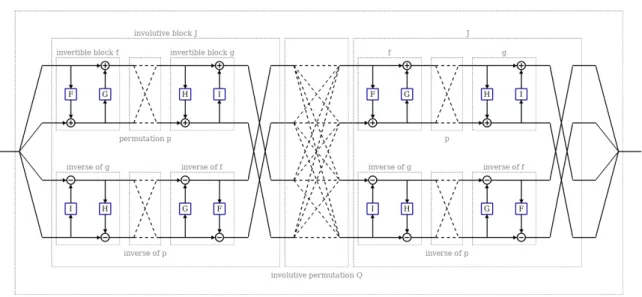
For a system diagram of the architecture for a typical involutive neural network, see Fig. 2.3.
Example deep involutive network
Figure 2.3: System diagram of a typical deep involutive network. The functions 𝐹 , 𝐺,
𝐻, and 𝐼 are arbitrary functions, usually induced by neural networks.
2.4
Universality of Involutive Generative Models
When using a machine learning model, it is useful to know which class of functions the model can represent. In this section, we consider generative models built from deep involutive networks, and show that they are universal approximators in a certain sense. Specifically, we prove that these networks, which map a state and an auxiliary variable (𝜑, 𝜋) ∈ (R𝑛, R𝑚) to an output interpreted as another state and auxiliary
variable (𝜑′, 𝜋′), can serve as arbitrarily good generative models of any continuous function of a Gaussian on any compact subset of R𝑛.
The theorem statement and proof are given in Section 2.4.1.
Our proof is constructive: for any desired transition 𝑇 , we explicitly construct an involutive generative model such that transitions drawn from it are likely to be drawn, with arbitrarily high probability, from a distribution as close as desired to that of 𝑇 . Moreover, both of these approximation parameters are explicit in the description of the generative model. We first describe a family of involutive functions that approximate
the desired cumulative distribution function, and then make use of the universal approximation theorem [40], which has a constructive proof, to approximate these involutive functions by involutive neural nets.
As a consequence, involutive generative models simply match the expressive power of traditional neural generative models. There is, however, one key advantage: a standard generative model maps a state and auxiliary variable to a state: (𝜑, 𝜋) ↦→ 𝜑′, whereas an involutive generative model produces an additional piece of information, an output auxiliary variable 𝜋′ such that the model maps (𝜑′, 𝜋′) ↦→ (𝜑, 𝜋).
In other words, it produces a value for the auxiliary variable such that the model makes a backwards transition 𝜑′ ↦→ 𝜑. This immediately gives a lower bound on the backward transition probability (via the sampling distribution for 𝜋), and is a key property we use to easily generate Metropolis–Hastings transitions satisfying detailed balance as shown in Section 2.4.2.
2.4.1
Proof of Universality
Theorem 2.6 Involutive generative models are universal.
Let 𝑛 ∈ N, and let random variables 𝜋 ∼ 𝑁 (0𝑛+6, Id𝑛+6) and 𝜋′ ∼ 𝑁 (0, 1).
For all compact sets Ω ⊆ R𝑛, and all continuous functions 𝑇 : R𝑛× R → Ω there exists
a sequence {ℐ̂︀𝑚}𝑚∈N of involutive neural networks that induce continuous functions R2𝑛+6 → R2𝑛+6 such that for all 𝜑 ∈ Ω the random variables ℐ̂︀𝑚[𝜑] := ℐ̂︀𝑚(𝜑⌢𝜋)1..𝑛
converge in distribution to 𝑇 [𝜑] := 𝑇 (𝜑⌢𝜋′), as 𝑚 → ∞.
We begin with an outline of the proof technique. For each 𝑚 ∈ N, we aim to define a involutive neural network ℐ̂︀𝑚. We begin by exhibiting an involutive function parameterized by a positive real 𝜖𝑚 < 1 depending on 𝑚, such that when the auxiliary
variable is treated as a random variable, the involutive function matches the cumulative distribution function of the desired state transition arbitrarily well as 𝜖𝑚 → 0. Then
we show that this involutive function can be uniformly approximated arbitrarily well by an involutive neural network parameterized by some other positive real 𝛿𝑚 < 1
depending on both 𝜖𝑚 and 𝑚, as 𝛿𝑚 → 0. (In the main proof of Theorem 2.6below,
we will impose tighter constraints on 𝜖𝑚 and 𝛿𝑚.)
We will use Hornik’s Universal Approximation Theorem to obtain such a uniform approximation.
Theorem 2.7 Hornik [40, Thm. 3]
Let 𝑎, 𝑏 be positive integers, 𝐹 : R𝑎 → R𝑏
be a continuous function, and 𝜓 : R → R be a continuous bounded nonconstant activation function. For any compact set Ω ⊆ R𝑎
and 𝛿 > 0 there is a neural network consisting of a single hidden layer with activation 𝜓 that induces a continuous function 𝐹̂︀𝛿: R𝑎 → R𝑏 satisfying
max 𝑥∈Ω ⃒ ⃒ ⃒𝐹 (𝑥) −𝐹̂︀𝛿(𝑥) ⃒ ⃒ ⃒1 ≤ 𝛿.
We now define and prove several facts about some objects that will be useful in the proof. Define 𝑅𝜖𝑚: R 𝑛+3 → R𝑛+3 by 𝑅𝜖𝑚(𝑥) := ⎧ ⎪ ⎪ ⎪ ⎪ ⎪ ⎪ ⎪ ⎨ ⎪ ⎪ ⎪ ⎪ ⎪ ⎪ ⎪ ⎩ 0𝑛+3 if 𝑞 ≤ −1 2 (𝑞 + 1 2)(𝑇 (𝜑, 𝜋) − 𝜑) ⌢03 if −1 2 < 𝑞 < 1 2 (𝑇 (𝜑, 𝜋) − 𝜑)⌢03 if 1 2 ≤ 𝑞, where 𝜑 := 𝑥1..𝑛, 𝜋 := 𝑥𝑛+1𝜖𝑚 , and 𝑞 := 𝑥𝑛+3− 𝑥𝑛+2.
Define 𝑆 : R𝑛+3 → R𝑛+3 by 𝑆(𝑥) := ⎧ ⎪ ⎪ ⎪ ⎪ ⎪ ⎪ ⎪ ⎨ ⎪ ⎪ ⎪ ⎪ ⎪ ⎪ ⎪ ⎩ 0𝑛+3 if 𝑞 ≤ −12 (𝑞 + 12)𝜑′⌢03 if − 12 < 𝑞 < 12 𝜑′⌢03 if 12 ≤ 𝑞, where 𝜑′ := 𝑥1..𝑛 and 𝑞 := 𝑥𝑛+3− 𝑥𝑛+2. Define 𝑔𝜖𝑚: R 2𝑛+6 → R2𝑛+6 by 𝑔𝜖𝑚(𝑥) := 𝑥 ⊙ (1 𝑛⌢ 𝜖𝑚1𝑛+6) + (0𝑛+2⌢1⌢0𝑛+2⌢1),
where ⊙ denotes pointwise multiplication. Note that its inverse satisfies
𝑔𝜖−1𝑚(𝑥) = (𝑥 − (0𝑛+2⌢ 1⌢0𝑛+2⌢ 1)) ⊙ (1𝑛⌢ 1 𝜖𝑚1 𝑛+6). Define ℎ𝜖𝑚: R 2𝑛+6 → R2𝑛+6 by ℎ𝜖𝑚 := (︁ 𝑥1..𝑛+3+ 𝑆(𝑣) )︁⌢ 𝑣 where 𝑣 := 𝑥𝑛+4..2𝑛+6+ 𝑅𝜖𝑚(𝑥1..𝑛+3).
Note that its inverse satisfies
ℎ−1𝜖𝑚(𝑥) = 𝑤⌢(︁𝑥𝑛+4..2𝑛+6− 𝑅𝜖𝑚(𝑤)
)︁
where 𝑤 := 𝑥1..𝑛+3− 𝑆(𝑥𝑛+4..2𝑛+6).
Let 𝜎 be the permutation of {1, . . . , 2𝑛 + 6} that transposes 𝑛 + 2 with 𝑛 + 3 and transposes 2𝑛 + 5 with 2𝑛 + 6 (and leaves all other elements fixed).
Now consider the involutive function ℐ𝜖𝑚: R 2𝑛+6 → R2𝑛+6 defined by ℐ 𝜖𝑚 := 𝑔 −1 𝜖𝑚 ∘ ℎ−1𝜖𝑚 ∘ 𝐼𝑃2𝑛+6,𝜎∘ ℎ𝜖𝑚∘ 𝑔𝜖𝑚.
Let 𝐴𝜖𝑚 denote the event that 𝜋3− 𝜋2 > − 1 2𝜖𝑚 and 𝜋𝑛+6− 𝜋𝑛+5> − 1 2𝜖𝑚 and |𝜋| < 1 𝜖𝑚 all hold. Note that lim 𝜖𝑚→0 𝑃 (𝐴𝜖𝑚) = 1. (†)
Lemma 2.8 Conditioned on the event 𝐴𝜖𝑚, we have the following:
ℐ𝜖𝑚(𝜑
⌢
𝜋)1..𝑛 = 𝑇 (𝜑, 𝜋1) + 𝜖𝑚𝜋4..𝑛+3.
Proof. The event 𝐴𝜖𝑚 fully determines the branches of 𝑅𝜖𝑚 and 𝑆 that are taken in
the evaluation of ℐ𝜖𝑚(𝜑
⌢
𝜋), which enables us to simplify the expression ℐ𝜖𝑚(𝜑
⌢ 𝜋)1..𝑛
to the stated form.
For 𝜑 ∈ Ω, define the random variable ℐ𝜖𝑚[𝜑] := ℐ𝜖𝑚(𝜑
⌢
𝜋)1..𝑛. The following lemma is
immediate.
Lemma 2.9 Conditioned on the event 𝐴𝜖𝑚, the random variable ℐ𝜖𝑚[𝜑] converges in distribution to 𝑇 [𝜑] as 𝜖𝑚 → 0.
We will show that conditioned on the event 𝐴𝜖𝑚, and for appropriately small 𝜖𝑚 and 𝛿𝑚, we can approximate ℐ𝜖𝑚 arbitrarily well with an involutive neural networkℐ̂︀𝜖𝑚,𝛿𝑚.
Since Ω is a compact subset of R𝑛, it is bounded, and hence contained in a ball of finite radius 𝑟 ∈ R. Let Ω+⊆ R𝑛+3 be the closure of the ball of radius 7𝑟 + 10, and
let Ω++⊆ R𝑛+3 be the closure of the ball of radius 14𝑟 + 21. The sets Ω+ and Ω++ are closed and bounded, hence compact subsets of R𝑛+3.
Since 𝑅𝜖𝑚 and 𝑆 are continuous, by Theorem 2.7, for any 𝛿𝑚 > 0 there are neural
networks each with a single hidden layer and sigmoid activation that induce continuous functions 𝑅̂︀𝜖 𝑚,𝛿𝑚: R 𝑛+3 → R𝑛+3 and ̂︀ 𝑆𝛿𝑚: R 𝑛+3→ R𝑛+3, satisfying max 𝑥∈Ω++ ⃒ ⃒ ⃒𝑅𝜖𝑚(𝑥) −𝑅̂︀𝜖𝑚,𝛿𝑚(𝑥) ⃒ ⃒ ⃒1 ≤ 𝛿𝑚 and max 𝑥∈Ω++ ⃒ ⃒ ⃒𝑆(𝑥) −𝑆̂︀𝛿𝑚(𝑥) ⃒ ⃒ ⃒1 ≤ 𝛿𝑚. That is, 𝑅̂︀𝜖
𝑚,𝛿𝑚 and 𝑆̂︀𝛿𝑚 converge uniformly to 𝑅𝜖𝑚 and 𝑆, respectively, on Ω ++ as 𝛿𝑚 → 0. Defineℎ̂︀𝜖 𝑚,𝛿𝑚: R 2𝑛+6 → R2𝑛+6 by ̂︀ ℎ𝜖𝑚,𝛿𝑚 := (︁ 𝑥1..𝑛+3+𝑆̂︀𝛿 𝑚(𝑣 ′ ))︁⌢𝑣′ where 𝑣′ := 𝑥𝑛+4..2𝑛+6+𝑅̂︀𝜖 𝑚,𝛿𝑚(𝑥1..𝑛+3).
Note that its inverse satisfies
̂︀ ℎ−1𝜖𝑚,𝛿𝑚(𝑥) = 𝑤′⌢(︁𝑥𝑛+4..2𝑛+6−𝑅̂︀𝜖 𝑚,𝛿𝑚(𝑤 ′ ))︁ where 𝑤′ := 𝑥1..𝑛+3−𝑆̂︀𝛿 𝑚(𝑥𝑛+4..2𝑛+6).
Now form the involutive neural network that induces a functionℐ̂︀𝜖
𝑚,𝛿𝑚: R 2𝑛+6 → R2𝑛+6 defined as follows, ̂︀ ℐ𝜖𝑚,𝛿𝑚 := 𝑔 −1 𝜖𝑚 ∘̂︀ℎ −1 𝜖𝑚,𝛿𝑚∘ 𝐼 2𝑛+6,𝜎 𝑃 ∘ℎ̂︀𝜖𝑚,𝛿𝑚 ∘ 𝑔𝜖𝑚,
by composing the layers or neural nets corresponding to each term in the function definition.
Lemma 2.10 As 𝛿𝑚 → 0, the function ̂︀ℎ𝜖
𝑚,𝛿𝑚 converges uniformly to ℎ𝜖𝑚 on
Ω × 𝐵3(0𝑛+6) and its inverse ℎ̂︀−1
𝜖𝑚,𝛿𝑚 converges to ℎ −1
𝜖𝑚 on Ω
+× Ω+.
Proof. First observe that |𝑆(𝑥)| ≤ |𝑥| and |𝑅𝜖𝑚(𝑥)| ≤ 2𝑟, so that |ℎ𝜖𝑚(𝑥)| ≤ 3|𝑥| + 4𝑟.
For 𝑥 ∈ Ω × 𝐵3(0𝑛+6), we have |𝑥𝑛+4..2𝑛+6+𝑅̂︀𝜖
𝑚,𝛿𝑚(𝑥1..𝑛+3)| < |𝑅̂︀𝜖𝑚,𝛿𝑚(𝑥1..𝑛+3)| + 3 <
|𝑅𝜖𝑚(𝑥1..𝑛+3)| + 4 < 2𝑟 + 4, and hence we have 𝑥𝑛+4..2𝑛+6 +𝑅̂︀𝜖𝑚,𝛿𝑚(𝑥1..𝑛+3) ∈ Ω ++.
Thus for 𝑥 ∈ Ω × 𝐵3(0𝑛+6), all applications of 𝑅̂︀𝜖
𝑚,𝛿𝑚 and 𝑆̂︀𝛿𝑚 in ℎ̂︀𝜖𝑚,𝛿𝑚(𝑥) are on
points in Ω++ (where𝑅̂︀
𝜖𝑚,𝛿𝑚 and𝑆̂︀𝛿𝑚 converge uniformly to 𝑅𝜖𝑚 and 𝑆), and sô︀ℎ𝜖𝑚,𝛿𝑚
converges to ℎ𝜖𝑚 on Ω × 𝐵3(0
𝑛+6) as 𝛿
𝑚 → 0. Furthermore, the convergence is uniform,
since it is formed from sums and compositions of uniformly converging functions.
For 𝑥 ∈ Ω+ × Ω+ we have |𝑥
1..𝑛+3 −𝑆̂︀𝛿
𝑚(𝑥𝑛+4..2+6)| < |𝑆̂︀𝛿𝑚(𝑥𝑛+4..2+6)| + 7𝑟 + 10 <
|𝑆(𝑥𝑛+4..2+6)| + 7𝑟 + 11 < 14𝑟 + 21, and hence we have 𝑥𝑛+4..2𝑛+6−𝑆̂︀𝛿
𝑚(𝑥1..𝑛+3) ∈ Ω ++.
Thus for 𝑥 ∈ Ω+× Ω+, all applications of 𝑅̂︀
𝜖𝑚,𝛿𝑚 and𝑆̂︀𝛿𝑚 inℎ̂︀ −1
𝜖𝑚,𝛿𝑚(𝑥) are on points
in Ω++ (where𝑅̂︀𝜖
𝑚,𝛿𝑚 and𝑆̂︀𝛿𝑚 converge to 𝑅𝜖𝑚 and 𝑆) and sô︀ℎ −1 𝜖𝑚,𝛿𝑚 converges to ℎ −1 𝜖𝑚 on Ω+× Ω+ as 𝛿 𝑚 → 0.
Note that by Lemma 2.10, we have
max 𝑥∈Ω×𝐵1/𝜖𝑚(0𝑛+6) ⃒ ⃒ ⃒ ⃒ ̂︀ ℎ𝜖𝑚,𝛿𝑚(𝑔(𝑥)) − ℎ𝜖𝑚(𝑔(𝑥)) ⃒ ⃒ ⃒ ⃒< 1 (‡)
for sufficiently small 𝛿𝑚.
Lemma 2.11 Consider the random variable 𝑥 := 𝜑⌢𝜋. Conditioned on the event 𝐴𝜖𝑚, the function ℐ̂︀𝜖
𝑚,𝛿𝑚(𝑥) converges pointwise to ℐ𝜖𝑚(𝑥), as 𝛿𝑚 → 0.
Proof. Condition on 𝐴𝜖𝑚 and assume 𝛿𝑚is sufficiently small that (‡) holds. Then notice
that 𝑥 ∈ Ω×𝐵1/𝜖𝑚(0𝑛+6), so that 𝑔(𝑥) ∈ Ω×𝐵 3(0𝑛+6), and hence ⃒ ⃒ ⃒𝐼 2𝑛+6,𝜎 𝑃 (ℎ̂︀𝜖𝑚,𝛿𝑚(𝑔(𝑥))) ⃒ ⃒ ⃒= ⃒ ⃒ ⃒̂︀ℎ𝜖𝑚,𝛿𝑚(𝑔(𝑥)) ⃒ ⃒ ⃒< |ℎ𝜖𝑚(𝑔(𝑥))|+1 < 3|𝑔(𝑥)|+4𝑟+1 < 7𝑟+10. Thus 𝐼 2𝑛+6,𝜎 𝑃 (︁ ̂︀ ℎ𝜖𝑚,𝛿𝑚(𝑔(𝑥)) )︁ ∈ Ω+× Ω+. Hence when evaluating
̂︀
ℐ𝜖𝑚,𝛿𝑚(𝑥), the inputs to bothℎ̂︀𝜖𝑚,𝛿𝑚 and̂︀ℎ −1
the domains where their respective convergence properties stated in Lemma 2.10hold. Therefore each function occurring in the definition of ℐ̂︀𝜖
𝑚,𝛿𝑚 convergence pointwise to
the corresponding function in the definition of ℐ𝜖𝑚. Further, all such functions are
continuous, and so the result holds.
For 𝜑 ∈ Ω, define the random variable ℐ̂︀𝜖
𝑚,𝛿𝑚[𝜑] := ℐ̂︀𝜖𝑚,𝛿𝑚(𝜑
⌢
𝜋)1..𝑛. Let 𝜉𝑚 ∼
𝑁 (0𝑛, 𝜖𝑚Id𝑛) be an independently chosen Gaussian.
The following result is immediate from Lemma 2.11.
Lemma 2.12 Conditioned on the event 𝐴𝜖𝑚, the random variable ℐ̂︀𝜖𝑚,𝛿𝑚[𝜑] converges in distribution to ℐ𝜖𝑚[𝜑] as 𝛿𝑚 → 0.
We now prove Theorem 2.6.
Proof of Theorem 2.6. Fix 𝑚 ∈ N; we will defineℐ̂︀𝑚 such that the sequence {︁
̂︀ ℐ𝑚
}︁
𝑚∈N
has the desired convergence property using Lemmas2.9 and 2.12.
We may decompose the CDF of ℐ̂︀𝜖
𝑚,𝛿𝑚[𝜑] in terms of 𝐴𝜖𝑚 and ¯𝐴𝜖𝑚: 𝐹 ̂︀ ℐ𝜖𝑚,𝛿𝑚[𝜑](𝜑 ′ ) = 𝑃 (𝐴𝜖𝑚) · 𝐹 ̂︀ ℐ𝜖𝑚,𝛿𝑚[𝜑]|𝐴𝜖𝑚(𝜑 ′ ) + (1 − 𝑃 (𝐴𝜖𝑚)) · 𝐹 ̂︀ ℐ𝜖𝑚,𝛿𝑚[𝜑]| ¯𝐴𝜖𝑚(𝜑 ′ ).
Now we form a sequence {︁ℐ̂︀𝑚[𝜑] }︁
𝑚∈N and demonstrate that lim𝑚→∞𝐹̂︀ℐ𝑚[𝜑]
(𝜑′) =
𝐹𝑇 [𝜑](𝜑′) at all points of continuity 𝜑′ of 𝑇 [𝜑].
By Lemma 2.9 choose 𝜖𝑚 such that
|𝐹𝑇 [𝜑](𝜑′) − (𝐹ℐ𝜖𝑚[𝜑]|𝐴𝜖𝑚)(𝜑 ′
holds for all points of continuity 𝜑′ of 𝑇 [𝜑] and 𝑃 (𝐴𝜖𝑚) < 1
3𝑚 holds, which is possible
by (†).
By Lemma 2.12 choose 𝛿𝑚 so that
⃒ ⃒ ⃒(𝐹ℐ𝜖𝑚[𝜑]|𝐴𝜖𝑚)(𝜑 ′ ) − 𝐹 ̂︀ ℐ𝜖𝑚,𝛿𝑚[𝜑]|𝐴𝜖𝑚(𝜑 ′ )⃒⃒ ⃒< 1 3𝑚
holds for all points of continuity 𝜑′ of 𝑇 [𝜑] and (‡) holds. This is possible because conditioned on 𝐴𝜖𝑚, the random variable ℐ̂︀𝜖𝑚,𝛿𝑚[𝜑] converges in distribution to ℐ𝜖𝑚[𝜑]
and every point of continuity of 𝑇 [𝜑] is also a point of continuity of ℐ𝜖𝑚[𝜑].
Now define ℐ̂︀𝑚 :=ℐ̂︀𝜖
𝑚,𝛿𝑚. Observe that for any point of continuity 𝜑
′ of 𝑇 [𝜑], we have ⃒ ⃒ ⃒𝐹ℐ̂︀𝑚[𝜑](𝜑 ′ ) − 𝐹𝑇 [𝜑](𝜑′) ⃒ ⃒ ⃒ =⃒⃒ ⃒𝐹̂︀ℐ𝜖𝑚,𝛿𝑚[𝜑](𝜑 ′ ) − 𝐹𝑇 [𝜑](𝜑′) ⃒ ⃒ ⃒ <⃒⃒ ⃒𝐹̂︀ℐ𝜖𝑚,𝛿𝑚[𝜑]|𝐴𝜖𝑚(𝜑 ′ ) − 𝐹𝑇 [𝜑](𝜑′) ⃒ ⃒ ⃒+ 1 3𝑚 <⃒⃒ ⃒𝐹ℐ𝜖𝑚[𝜑]|𝐴𝜖𝑚(𝜑 ′ ) − 𝐹𝑇 [𝜑](𝜑′) ⃒ ⃒ ⃒+ 2 3𝑚 < 𝑚1.
Finally, considering this fact for all 𝑚 ∈ N, we see that ℐ̂︀𝑚[𝜑] converges in distribution to 𝑇 [𝜑].
Observe that universality holds even for the special case of volume-preserving involutive networks: the architecture ℐ̂︀𝜖
𝑚,𝛿𝑚 used in the constructive proof, defined by
̂︀ ℐ𝜖𝑚,𝛿𝑚 := 𝑔 −1 𝜖𝑚 ∘̂︀ℎ −1 𝜖𝑚,𝛿𝑚∘ 𝐼 2𝑛+6,𝜎 𝑃 ∘ℎ̂︀𝜖 𝑚,𝛿𝑚 ∘ 𝑔𝜖𝑚,
has a Jacobian whose determinant has magnitude 1, sinceℎ̂︀𝜖
𝑚,𝛿𝑚 has the structure of
an additive coupling layer and the constant Jacobians of 𝑔𝜖−1𝑚 and 𝑔𝜖𝑚 cancel.
models, we now review the following known result showing that volume-preserving involutive functions can be used as valid proposals within an MCMC algorithm.
2.4.2
Volume-preserving involutive functions lead to Metropolis–
Hastings proposals satisfying detailed balance
The proof of detailed balance for Hybrid Monte Carlo relies on the fact that Hamiltonian dynamics composed with negating momentum is involutive and volume-preserving. It is also known that volume-preserving involutive functions lead to Metropolis–Hastings proposals satisfying detailed balance (see, e.g., [23]), but we were unable to find a published argument. For completeness we describe here a procedure for using any volume-preserving involutive function as a proposal, and prove its correctness.
Our goal is to use a volume-preserving involutive function 𝑓𝜃 to construct a Markov
process with 𝑃𝑆(𝜑) as a stationary distribution. To do this, we will find a transition
such that the transition probabilities 𝑃𝑀(𝜑 ↦→ 𝜑′) satisfy the detailed balance condition
𝑃𝑆(𝜑)𝑃𝑀(𝜑 ↦→ 𝜑′) = 𝑃𝑆(𝜑′)𝑃𝑀(𝜑′ ↦→ 𝜑).
We follow the original derivation of Hybrid Monte Carlo [29], since the structure of the proof is similar.
In order to make a transition, we do the following.
1. Introduce an auxiliary random variable 𝜋 with probability density 𝑃𝐺.
volume-preserving involutive function 𝑓𝜃:
𝑃𝐻((𝜑, 𝜋) ↦→ (𝜑′, 𝜋′)) = 𝛿[(𝜑′, 𝜋′) − 𝑓𝜃((𝜑, 𝜋))].
3. Accept or reject that transition according to the Metropolis–Hastings acceptance criterion 𝑃𝐴((𝜑, 𝜋) ↦→ (𝜑′, 𝜋′)) = min (︂ 1,𝑃𝑆(𝜑 ′)𝑃 𝐺(𝜋′)𝑃𝐻((𝜑′, 𝜋′) ↦→ (𝜑, 𝜋)) 𝑃𝑆(𝜑)𝑃𝐺(𝜋)𝑃𝐻((𝜑, 𝜋) ↦→ (𝜑′, 𝜋′)) )︂ .
4. Marginalize over the auxiliary variable 𝜋.
Formally, we define our transition probability by
𝑃𝑀(𝜑 ↦→ 𝜑′) = ∫︁ (︂ 𝑃𝐺(𝜋) 𝑃𝐻((𝜑, 𝜋) ↦→ (𝜑′, 𝜋′)) 𝑃𝐴((𝜑, 𝜋) ↦→ (𝜑′, 𝜋′)) )︂ 𝑑𝜋𝑑𝜋′.
We now show that this transition satisfies the detailed balance condition.
Lemma 2.13 Applying 𝑓𝜃 within a Dirac 𝛿 distribution leaves the 𝛿 unchanged:
𝛿[𝑥 − 𝑦] = 𝛿[𝑓𝜃(𝑥) − 𝑓𝜃(𝑦)]
Proof. For arbitrary 𝐹 we have
𝐹 (𝑦) =
∫︁
Ω
and ∫︁ Ω 𝛿[𝑓𝜃(𝑥)−𝑓𝜃(𝑦)]𝐹 (𝑥) 𝑑𝑥 = ∫︁ 𝑓𝜃(Ω) 𝛿[𝑢 − 𝑓𝜃(𝑦)]𝐹 (𝑓𝜃−1(𝑢)) 𝑑𝑢 | det 𝑓′ 𝜃(𝑥)| = ∫︁ 𝑓𝜃(Ω) 𝛿[𝑢 − 𝑓𝜃(𝑦)]𝐹 (𝑓𝜃−1(𝑢)) 𝑑𝑢
(since 𝑓𝜃 preserves volume)
= 𝐹 (𝑓𝜃−1(𝑓𝜃(𝑦))) = 𝐹 (𝑦), and so ∫︁ Ω 𝛿[𝑥 − 𝑦]𝐹 (𝑥) 𝑑𝑥 = ∫︁ Ω 𝛿[𝑓 (𝑥) − 𝑓 (𝑦)]𝐹 (𝑥) 𝑑𝑥. Hence 𝛿[𝑥 − 𝑦] = 𝛿[𝑓 (𝑥) − 𝑓 (𝑦)]. Lemma 2.14 𝑃𝐻 is symmetric: 𝑃𝐻((𝜑, 𝜋) ↦→ (𝜑′, 𝜋′)) = 𝑃𝐻((𝜑′, 𝜋′) ↦→ (𝜑, 𝜋)). Proof. We have 𝑃𝐻((𝜑, 𝜋) ↦→ (𝜑′, 𝜋′)) = 𝛿[(𝜑′, 𝜋′) − 𝑓𝜃((𝜑, 𝜋))] = 𝛿[𝑓𝜃((𝜑′, 𝜋′)) − 𝑓𝜃∘ 𝑓𝜃((𝜑, 𝜋))] (by Lemma 2.13) = 𝛿[𝑓𝜃((𝜑′, 𝜋′)) − (𝜑, 𝜋)] (since 𝑓𝜃 is involutive) = 𝛿[(𝜑, 𝜋) − 𝑓𝜃((𝜑′, 𝜋′))] (since 𝛿[𝑥] = 𝛿[−𝑥]) = 𝑃𝐻((𝜑′, 𝜋′) ↦→ (𝜑, 𝜋)),
establishing the lemma.
Lemma 2.15 𝑃𝐴 satisfies the following simpler form:
𝑃𝐴((𝜑, 𝜋) ↦→ (𝜑′, 𝜋′)) = min (︂ 1,𝑃𝑆(𝜑 ′)𝑃 𝐺(𝜋′) 𝑃𝑆(𝜑)𝑃𝐺(𝜋) )︂ .
Proof. Apply Lemma 2.14 to the definition of 𝑃𝐴.
Lemma 2.16 𝑃𝑆𝑃𝐺𝑃𝐴 is symmetric: 𝑃𝑆(𝜑)𝑃𝐺(𝜋)𝑃𝐴((𝜑, 𝜋) ↦→ (𝜑′, 𝜋′)) = 𝑃𝑆(𝜑′)𝑃𝐺(𝜋′)𝑃𝐴((𝜑′, 𝜋′) ↦→ (𝜑, 𝜋)). Proof. We have 𝑃𝑆(𝜑)𝑃𝐺(𝜋)𝑃𝐴((𝜑, 𝜋) ↦→ (𝜑′, 𝜋′)) = 𝑃𝑆(𝜑)𝑃𝐺(𝜋) min (︂ 1,𝑃𝑆(𝜑 ′)𝑃 𝐺(𝜋′) 𝑃𝑆(𝜑)𝑃𝐺(𝜋) )︂ = min(︁𝑃𝑆(𝜑)𝑃𝐺(𝜋), 𝑃𝑆(𝜑′)𝑃𝐺(𝜋′) )︁ = 𝑃𝑆(𝜑′)𝑃𝐺(𝜋′) min (︂ 𝑃 𝑆(𝜑)𝑃𝐺(𝜋) 𝑃𝑆(𝜑′)𝑃𝐺(𝜋′) , 1 )︂ = 𝑃𝑆(𝜑′)𝑃𝐺(𝜋′)𝑃𝐴((𝜑′, 𝜋′) ↦→ (𝜑, 𝜋)), as desired.
Theorem 2.17 The Markov chain defined by transitions 𝑃𝑀 has 𝑃𝑆 as a stationary
distribution.
Proof. It suffices to show that 𝑃𝑀 satisfies the detailed balance condition
We have 𝑃𝑆(𝜑)𝑃𝑀(𝜑 ↦→ 𝜑′) = ∫︁ (︂ 𝑃𝑆(𝜑)𝑃𝐺(𝜋)𝑃𝐻((𝜑, 𝜋) ↦→ (𝜑′, 𝜋′)) 𝑃𝐴((𝜑, 𝜋) ↦→ (𝜑′, 𝜋′)) )︂ 𝑑𝜋𝑑𝜋′ = ∫︁ (︂ 𝑃𝑆(𝜑′)𝑃𝐺(𝜋′)𝑃𝐻((𝜑, 𝜋) ↦→ (𝜑′, 𝜋′)) 𝑃𝐴((𝜑′, 𝜋′) ↦→ (𝜑, 𝜋)) )︂ 𝑑𝜋𝑑𝜋′ (by Lemma 2.16) = ∫︁ (︂ 𝑃𝑆(𝜑′)𝑃𝐺(𝜋′)𝑃𝐻((𝜑′, 𝜋′) ↦→ (𝜑, 𝜋)) 𝑃𝐴((𝜑′, 𝜋′) ↦→ (𝜑, 𝜋)) )︂ 𝑑𝜋𝑑𝜋′ (by Lemma 2.14) = 𝑃𝑆(𝜑′)𝑃𝑀(𝜑′ ↦→ 𝜑), and so (⋆) holds.
We have established that for Markov processes generated by our transition, the desired distribution is stationary, by showing that it satisfies detailed balance. This implies, when the chain is ergodic, that the MCMC procedure eventually generates samples which are arbitrarily close in total variation distance to the posterior distribution.
2.5
Training and sampling algorithm
Having established the generality of our involutive MCMC procedure, we now describe a method for training optimized involutive transition kernels.
As discussed in [101], a useful transition kernel satisfies three criteria: 1) low bias in the limit; 2) fast convergence; and 3) low autocorrelation.