HAL Id: hal-00457234
https://hal.archives-ouvertes.fr/hal-00457234
Submitted on 16 Feb 2010
HAL is a multi-disciplinary open access
archive for the deposit and dissemination of
sci-entific research documents, whether they are
pub-lished or not. The documents may come from
teaching and research institutions in France or
abroad, or from public or private research centers.
L’archive ouverte pluridisciplinaire HAL, est
destinée au dépôt et à la diffusion de documents
scientifiques de niveau recherche, publiés ou non,
émanant des établissements d’enseignement et de
recherche français ou étrangers, des laboratoires
publics ou privés.
Stéphane Gosselin, Guillaume Damiand, Christine Solnon
To cite this version:
Stéphane Gosselin, Guillaume Damiand, Christine Solnon. Signatures of combinatorial maps. 13th
In-ternational Workshop on Combinatorial Image Analysis (IWCIA), Nov 2009, Cancun, Mexico.
pp.370-382. �hal-00457234�
St´ephane Gosselin1 and Guillaume Damiand1and Christine Solnon1⋆
Universit´e de Lyon, CNRS
Universit´e Lyon 1, LIRIS, UMR5205, F-69622, France
{stephane.gosselin,guillaume.damiand,christine.solnon}@liris.cnrs.fr
Abstract. In this paper, we address the problem of computing a canon-ical representation of an n-dimensional combinatorial map. To do so, we define two combinatorial map signatures: the first one has a quadratic space complexity and may be used to decide of isomorphism with a new map in linear time whereas the second one has a linear space complexity and may be used to decide of isomorphism in quadratic time. Experimen-tal results show that these signatures can be used to recognize images very efficiently.
Key words: Combinatorial map, canonical representation, signature, linear isomorphism
1
Motivations
Combinatorial maps are good data structures for modelling space subdivisions. First defined in 2D [7, 16, 9, 3], they have been extended to nD [2, 11, 12] and model the subdivision cells and their adjacency relations in any dimension.
There are many different data structures for modelling the partition in regions of an image. All these structures are more or less derived from Region Adjacency Graphs (RAG) [15]. It has been shown that using combinatorial maps allows a precise description of the topology of the image partition (for example in 2D [1] or in 3D [4]) and there are efficient image processing algorithms using this topological information .
Our general goal is to define new algorithms for combinatorial maps allow-ing new and efficient image processallow-ing algorithms. Among these operations, we are interested in image classification. In particular, we propose to characterize image classes by extracting patterns which occur frequently in these classes. When modelling images with combinatorial maps, this involves finding frequent submaps. Finding frequent patterns in large databases is a classical data mining problem, the tractability of which highly depends on the existency of efficient algorithms for deciding if two patterns are actually different or if they are two occurrences of a same object. Hence, if finding frequent subgraphs is intractable in the general case, it may be solved in incremental polynomial time when con-sidering classes of graphs for which subgraph isomorphism may be solved in polynomial time, such as trees or outerplanar graphs [8].
⋆
The authors acknowledge an Anr grant Blanc 07-1 184534: this work was done in the context of project Sattic.
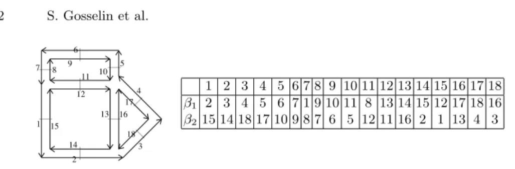
7 9 11 12 6 13 16 8 10 5 4 17 18 3 14 2 15 1 1 2 3 4 5 6 7 8 9 10 11 12 13 14 15 16 17 18 β1 2 3 4 5 6 7 1 9 10 11 8 13 14 15 12 17 18 16 β215 14 18 17 10 9 8 7 6 5 12 11 16 2 1 13 4 3
Fig. 1. Combinatorial map example. Darts are represented by numbered black seg-ments. Two darts 1-sewn are drawn consecutively, and two darts 2-sewn are concur-rently drawn and in reverse orientation, with little grey segment between the two darts.
In this paper, we address the problem of computing a canonical represen-tation of combinatorial maps which may be used to efficiently search a map in a database. This work may be related to [10], which proposes a polynomial al-gorithm for deciding of the isomorphism of ordered graphs, based on a vertex labelling. Recently, this work has been extended to deal with combinatorial maps by proposing a polynomial algorithm for map and submap isomorphism based on a traversal of the map [6]. We use these principles of labelling and traversal to define canonical representations of combinatorial maps.
More precisely, we define two map signatures. Both signatures may be com-puted in quadratic time with respect to the number of darts of the map. The first signature is a lexicographic tree and has a quadratic space complexity. It allows one to decide in linear time if a new map is isomorphic to a map described by this signature. The second signature is a word and has a linear space complexity. As a counterpart, isomorphism with a new map becomes quadratic.
Notions of combinatorial maps are introduced in section 2. Section 3 presents an algorithm for labelling maps. Two signatures for connected maps are defined in section 4 and section 5. These signatures are extended to non connected maps in section 6. Finally, we experimentally evaluate our work in section 7.
2
Recalls on Combinatorial Maps
Definition 1 (Combinatorial map [12]). An nD combinatorial map, (or n-map) is defined by a tuple M = (D, β1, . . . , βn) where
– D is a finite set of darts;
– β1 is a permutation on D, i.e., a one-to-one mapping from D to D; – ∀ 2 ≤ i ≤ n, βi is an involution on D, i.e., a one-to-one mapping from D to
D such that βi= β−1i ;
– ∀ 1 ≤ i ≤ n − 2, ∀ i + 2 ≤ j ≤ n, βi◦ βj is an involution on D.
We note β0 for β1−1. Two darts i and j such that i = βk(j) are said to be k-sewn. Fig. 1 gives an example of a 2D combinatorial map.
In some cases, it may be useful to allow some βito be partially defined, thus leading to open combinatorial maps. The basic idea is to add a new element ǫ to
f a b d g c e a b c d e f g β1b c d a f g e β2 ǫ ǫ e ǫ c ǫ ǫ
Fig. 2.Open combinatorial map example. Darts a, b, d, f and g are not 2-sewn.
the set of darts, and to allow darts to be i-sewn with ǫ. By definition, ∀0 ≤ i ≤ n, βi(ǫ) = ǫ. Fig. 2 gives an example of open map (see [14] for precise definitions). Lienhardt has defined isomorphism between two combinatorial maps as fol-lows.
Definition 2 (Map isomorphism [13]). Two maps M = (D, β1, . . . , βn) and M′ = (D′, β′
1, . . . , βn) are isomorphic if there exists a one-to-one mapping′ f : D → D′, called isomorphism function, such that ∀d ∈ D, ∀i, 1 ≤ i ≤ n f(βi(d)) = β′
i(f (d)).
This definition has been extended to open maps in [6] by adding that f (ǫ) = ǫ, thus enforcing that, when a dart is i-sewn with ǫ, then the dart matched to it by f is i-sewn with ǫ.
Finally, Def. 3 states that a map is connected if there is a path of sewn darts between every pair of darts.
Definition 3 (Connected map). A combinatorial map M = (D, β1, . . . , βn) is connected if ∀d ∈ D, ∀d′∈ D, there exists a path (d1, . . . , dk) such that d1= d, dk= d′ and ∀1 ≤ i < k, ∃ji∈ {0, . . . , n}, di+1= βj
i(di).
3
Map Labelling
Our signatures are based on map labellings, which associate a different label with every different dart. By definition, the label associated with ǫ is 0.
Definition 4 (Labelling). Given a map M = (D, β1, . . . , βn) a labelling of M is a bijective function l : D ∪ {ǫ} → {0, . . . , |D|} such that l(ǫ) = 0.
Example 1. l = {ǫ : 0, a : 3, b : 1, c : 5 , d : 7, e : 2, f : 6, g : 4} is a labelling of the map displayed in Fig. 2.
One may compute a labelling of a map by performing a map traversal and labelling darts with respect to the order of their discovery. Different labellings may be computed, depending on (i) the initial dart from which the traversal is started, (ii) the strategy used for memorizing the darts that have been discovered but that have not yet been used to discover new darts (e.g., FIFO or LIFO), and (iii) the order in which the βi functions are used to discover new darts.
We define below the labelling corresponding to a breadth first traversal of a map where βi functions are used in increasing order.
Algorithm 1: BF L(M, d)
Input: an open connected map M = (D, β1, . . . , βn), and a dart d ∈ D
Output: a labelling l : D ∪ {ǫ} → {0, . . . , |D|} foreach d′∈ D do l(d′) ← −1
1
l(ǫ) ← 0
2
let Q be an empty queue
3
add d at the end of Q
4
l(d) ← 1
5
nextLabel ← 2
6
while Qis not empty do
7
remove d′ from the head of Q
8 for iin 0 . . . n do 9 if l(βi(d′)) = −1 then 10 l(βi(d′)) ← nextLabel 11 nextLabel ← nextLabel + 1 12
add βi(d′) at the end of Q
13
return l
14
Definition 5 (Breadth first labelling (BFL)). Given a connected map M = (D, β1, . . . , βn) and a dart d ∈ D the breadth first labelling associated with (M, d) is the labelling returned by the function BF L(M, d) described in algorithm 1.
Example 2. The breadth first labellings associated with the map of Fig. 2 for darts a and e respectively are
BF L(M, a) = {ǫ : 0, a : 1, b : 3, c : 4, d : 2, e : 5, f : 7, g : 6} BF L(M, e) = {ǫ : 0, a : 7, b : 5, c : 4, d : 6, e : 1, f : 3, g : 2} Proposition 1. Algorithm 1 returns a labelling.
Proof.
– l(ǫ) is set to 0 in line 2.
– ∀d, d′ ∈ D, d 6= d′ ⇒ l(d) 6= l(d′). Indeed, each time a label is assigned to a dart (line 11), nextLabel is incremented (line 12).
– ∀d ∈ D, 1 ≤ l(d) ≤ |D|. Indeed, each dart enters exactly once in the queue because (i) the map is connected and (ii) a dart enters the queue only if it has not yet been labelled, and it is labelled just before entering it. ⊓⊔ Proposition 2. The time complexity of algorithm 1 is O(n · |D|)
Proof. The while loop (line 7-13) is iterated |D| times as (i) exactly one dart d is removed from the queue at each iteration; and (ii) each dart d ∈ D enters the queue exactly once. The for loop (lines 9-13) is iterated n + 1 times. ⊓⊔
Given a map M and a labelling l, one may describe M (i.e., its functions β1 to βn) by a sequence of labels of l. The idea is to first list the n labels of the n darts which are i-sewn with the dart labelled by 1 (i.e., l(β1(1)), . . . , l(βn(1))), and then by 2 (i.e., l(β1(2)), . . . , l(βn(2))), etc. More formally, we define the word associated with a map and a labelling as follows.
Definition 6 (Word). Given a connected map M = (D, β1, . . . , βn) and a la-belling l : D ∪ {ǫ} → {0, . . . , |D|} the word associated with (M, l) is the sequence
W(M, l) =< w1, . . . , wn·|D|>
such that ∀i ∈ {1, . . . , n}, ∀k ∈ {1, . . . , |D|}, wi·k = l(βi(dk)) where dk is the dart labelled with k, i.e., dk= l−1(k).
Algorithm. Given a map M = (D, β1, . . . , βn) and a labelling l, the word W (M, l) is computed by considering every dart of D in increasing label order and enu-merating the labels of its n i-sewn darts. This is done in O(n · |D|).
Notation. The word associated with the breadth first labelling of a map M , starting from a dart d, is denoted by WBF L(M, d), i.e.,
WBF L(M, d) = W (M, BF L(M, d))
Example 3. The words associated with the map of Fig. 2 for the two labellings of example 2 respectively are
WBF L(M, a) =< 3, 0, 1, 0, 4, 0, 2, 5, 7, 4, 5, 0, 6, 0 > WBF L(M, e) =< 3, 4, 1, 0, 2, 0, 6, 1, 4, 0, 7, 0, 5, 0 >
The key point which allows us to use words for building signatures is that two maps are isomorphic if and only if they share a word for a breadth first labelling, as stated in theorem 1.
Theorem 1. Two connected maps M = (D, β1, . . . , βn) and M′= (D′, β1, . . . , β′ ′ n) are isomorphic iff there exist d ∈ D and d′ ∈ D′ such that WBF L(M, d) = WBF L(M′, d′)
Proof. ⇒ Let us first consider two isomorphic maps M = (D, β1, . . . , βn) and M′ = (D′, β′
1, . . . , βn), and let us show that there exist two darts d and d′ ′ such that WBF L(M, d) = WBF L(M′, d′). If M and M′ are isomorphic then there exists f : D → D′ such that ∀d ∈ D, ∀i ∈ {1, . . . , n}, f (βi(d)) = βi(f (d)).′ Let d1 be a dart of D, and let us note l (resp. l′) the labellings returned by BF L(M, d1) (resp. BF L(M′, f(d1))). Claim 1: l and l′ are such that ∀di ∈ D, l(di) = l′(f (di)). This is true for the initial dart d1 as both d1 and f (d1) are labelled with 1 at the beginning of each traversal. This is true for every other dart di ∈ D as the traversals of M and M′ performed by BF L are completely determined by the fact that (i) they consider the same FIFO strategy to select the next labelled dart which will be used to discover new darts and (ii) they
use the βi functions in the same order to discover new darts from a selected labelled dart. Claim 2: ∀k ∈ {1, . . . , |D|}, f (l−1(k)) = l′−1(k). This is a direct consequence of Claim 1. Conclusion: ∀i ∈ {1, . . . , n}, ∀k ∈ {1, . . . , |D|}, the i.kth element of WBF L(M, d1) is equal to the i.kthelement of W′
BF L(M′, f(d1)), i.e., l(βi(l−1(k))) = l′(β′
i(l′−1(k))). Indeed,
l(βi(l−1(k))) = l′(f (βi(l−1(k)))) (because of Claim 1)
= l′(βi(f (l′ −1(k)))) (because f is an isomorphism function) = l′(β′
i(l′−1(k))) (because of Claim 2)
⇐ Let us now consider two maps M = (D, β1, . . . , βn) and M′ = (D′, β1, . . . , β′ ′ n) and two darts d and d′ such that WBF L(M, d) = WBF L(M′, d′), and let us show that M and M′ are isomorphic. Let us note l (resp. l′) the labellings returned by BF L(M, d) (resp. BF L(M′, d′)), and let us define the function f : D → D′ which matches darts with same labels, i.e., ∀dj ∈ D, f (dj) = l′−1(l(dk)). Note that this implies as well that l(dj) = l′(f (dj)). Claim 3: ∀i ∈ {1, . . . , n}, ∀k ∈ {1, . . . , |D|}, l(βi(l−1(k))) = l′(β′
i(l′−1(k))). This comes from the fact that WBF L(M, d) = WBF L(M′, d′) so that the i.kthelement of WBF L(M, d1) is equal to the i.kthelement of W′
BF L(M′, f(d1)). Conclusion: ∀i ∈ {1, . . . , n}, ∀dj∈ D,
f(βi(dj)) = l′−1(l(βi(dj))) (by definition of f ) = l′−1(l′(β′ i(l′−1(l(dj))))) (because of Claim 3) = βi′(l′−1(l(dj))) (by simplification) = β′ i(l′−1(l′(f (dj)))) (by definition of f ) = β′i(f (dj)) (by simplification)
Hence, f is an isomorphism function and M and M′ are isomorphic. ⊓⊔
4
Set Signature of a Connected Map
A map is characterized by the set of words associated with all possible breadth first labellings. This set defines a signature.
Definition 7 (Set Signature). Given a map M = (D, β1, . . . , βn) the Set Signature associated with M is SS(M ) = {WBF L(M, d)|d ∈ D}
Algorithm. SS(M ) is built by performing WBF L(M, d) for each d ∈ D and col-lecting all different returned words in SS(M ). Hence, the overall time complexity is O(n · |D|2).
Theorem 2. SS(M ) is a signature, i.e., two connected maps M and M′ are isomorphic if and only if SS(M ) = SS(M′)
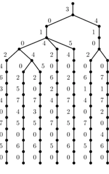
Fig. 3.Lexicographical tree of the set signature of the map of Fig. 2.
Proof. ⇒ Let us consider two isomorphic maps M = (D, β1, . . . , βn) and M′= (D′, β1, . . . , β′ ′
n), and let us show that SS(M ) = SS(M′). This is a direct con-sequence of theorem 1, where we have shown that given an isomorphism func-tion f between M and M′ we have, for every dart d ∈ D, WBF L(M, d) = WBF L(M′, f(d)). Hence, every word of SS(M ), computed from any dart of D, necessary belongs to SS(M′) (and conversely).
⇐ Let us consider two maps M = (D, β1, . . . , βn) and M′= (D′, β′ 1, . . . , β
′ n) such that SS(M ) = SS(M′), and let us show that M and M′ are isomorphic. Indeed, there exist two words W ∈ SS(M ) and W′ ∈ SS(M′) such that W = W′, thus M and M′ are isomorphic due to theorem 1. ⊓⊔ Note that a direct consequence of theorem 1 and theorem 2 is that for two non isomorphic maps M and M′, SS(M ) ∩ SS(M′) = ∅.
Property 1. The space complexity of the set signature of a map is O(n · |D|2). Proof. The set signature contains at most |D| words (it may contains less than |D| words in case of automorphisms). Each word contains exactly n · |D| labels. Lexicographical tree. The set signature of a map may be represented by a cographical tree which groups common prefixes of words. For example, the lexi-cographical tree of the set signature of the map displayed in Fig. 2 is displayed in Fig. 3.
Property 2. Given a map M = (D, β1, . . . , βn) and the lexicographical tree of the set signature SS(M′) of another map M′, one determine the isomorphism between M and M′ in O(n · |D|).
Proof. To decide of the isomorphism, one has to build a breadth first labelling, starting from any dart of d ∈ D, and check if WBF L(M, d) is a branch of the lexicographical tree. Note that a node of the tree may have more than one son but, as the number of branches of the tree is bounded by the number of darts, deciding if a breadth first labelling corresponds to a branch of the tree may be
done in linear time. ⊓⊔
5
Word Signature of a Connected Map
The lexicographical order is a strict total order on a set signature, and we have shown that if two set signatures share one word, then they are equal. Hence, one may define a map signature by considering the smallest word of the set signature. Definition 8 (Word Signature). Given a map M , the Word Signature of M is, W S(M ) = w ∈ SS(M ) such that ∀w′∈ SS(M ), w ≤ w′.
Example 4. The word signature of the map displayed in Fig. 2 is W S(M ) =< 3, 0, 1, 0, 2, 4, 6, 3, 4, 0, 7, 0, 5, 0 > Property 3. The space complexity of a word signature is O(n · |D|).
Algorithm. The word signature of a map M is built by calling WBF L(M, d) for each dart d ∈ D, and keeping the smallest returned word with respect to the lexicographical order. The time complexity for computing the word signa-ture is O(n · |D|2). Note that this process may be improved (without changing the worst case complexity) by incrementally comparing the word in construc-tion with the current smallest word and stopping the construcconstruc-tion as soon as it becomes greater.
Property 4. Given a map M = (D, β1, . . . , βn) and the word signature W S(M′) of another map M′, one determine the isomorphism between M and M′ in O(n · |D|2).
Proof. To decide of the isomorphism, one has to build breadth first labellings, starting from every different dart of d ∈ D, and check if WBF L(M, d) = W S(M′). In the worst case, one has to build |D| labellings so that the overall time com-plexity is in O(n · |D|2). ⊓⊔
6
Signatures of Non Connected Maps
When a map is not connected, it may be decomposed in a set of disjoint con-nected maps in linear time with respect to the number of darts by performing successive map traversals until all darts have been discovered. The signature of a non connected map is built from the signatures of its different connected components.
Fig. 4.Example of non connected map and its Set Signature.
Word signature. To build a signature from the word signatures of the connected components, we sort the signatures by lexicographical order to obtain a list of words.
Set signature. To build a signature from the set signatures of the connected components, we merge the lexicographical trees as displayed in Fig. 4. Each node in the merged tree corresponding to a leaf in the tree of the ithconnected component is labelled by i. Note that a node in the merged tree may have several labels as some connected components may be isomorphic. Note also that labelled nodes in the merged tree may be internal nodes as a branch of the tree of a connected component may be a prefix of the branch of another tree. To decide isomorphism between a non connected map and a Set Signature, we have to compute a breadth first labelling of each connected component starting from any dart, and check that each corresponding word ends in a node of the merged tree which is labelled by a different connected component.
7
Experiments
Using map signatures to search images. Maps may be extracted from segmented images by using the linear algorithm described in [5]. We obtain the same map whatever we submit the image to a rotation or a scale-up. Hence, map signatures may be used to identify images even if they have been rotated or scaled-up. Table 1 shows 5 images and gives the number of darts and faces of maps extracted from these images, and then gives the CPU time needed to compute set and word signatures. Image Darts 3410 6060 1728 4224 1590 Faces 590 1044 295 716 275 SS(M ) 0.83 2.21 0.26 1.14 0.26 W S(M ) 0.26 0.53 0.15 0.32 0.16
Table 1.From images to signatures: the first line displays images, the next two lines give the number of darts and faces in the corresponding maps; the last two lines give the CPU time in seconds for computing the set and word signatures of these maps.
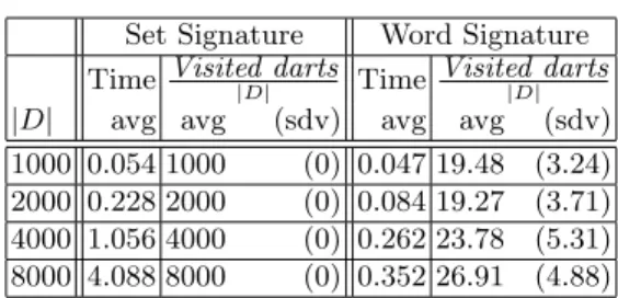
Set Signature Word Signature Time Visited darts|D| Time Visited darts|D|
|D| avg avg (sdv) avg avg (sdv)
1000 0.054 1000 (0) 0.047 19.48 (3.24)
2000 0.228 2000 (0) 0.084 19.27 (3.71)
4000 1.056 4000 (0) 0.262 23.78 (5.31)
8000 4.088 8000 (0) 0.352 26.91 (4.88)
Table 2. Comparison of time complexities for computing set and word signatures of a map. Each line successively gives the number of darts |D| of the map and, for each signature, the CPU time (in seconds) and the ratio between the number of visited darts and |D|. We give average results (and standard deviations) obtained with different initial darts.
Scale-up properties of signature constructions. To compare scale-up properties of set and word signatures, we have performed experiments on randomly gen-erated maps with exponentially growing sizes (with 1000, 2000, 4000 and 8000 darts). Table 2 first compares time complexities for constructing set and word signatures. To build the set signature, one has to perform a complete breadth first traversal for each dart so that the total number of visited darts is always equal to |D|2 and the time complexity does not depend on the initial dart cho-sen to start the traversal. To build a word signature, one also has to perform a breadth first traversal for each dart but each traversal may be stopped as soon as the corresponding word is greater than the smallest word computed so far. Hence, if the worst case complexity is quadratic, Table 2 shows that the CPU time needed to compute a word signature is sub quadratic in practice. Indeed, the average number of darts visited for each traversal varies from 19.48 for the map with 1000 darts to 26.91 for the map with 8000 darts. Note that, if the number of visited darts actually depends on the order in which initial darts are chosen, standard deviations are rather low.
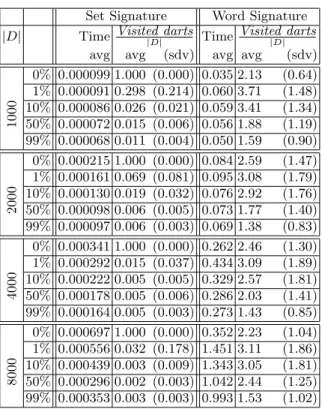
Scale-up properties of isomorphism. We now compare set and word signatures for deciding if a new map M′ is isomorphic to a map M described by its signature. When using the set signature SS(M ), the worst case complexity is O(n·|D|). Table 3 shows that, when M′ and M are isomorphic (when the percentage of different darts is 0%), the algorithm visits each dart exactly once. However, when M and M′ are not isomorphic, the breadth first traversal of M′ may be stopped as soon as no branch of the lexicographical tree matches the word under construction. Table 3 shows that the more different M and M′, the smaller the number of visited darts.
When using the word signature W S(M ), the worst case complexity is O(n · |D|2) as one has to perform a breadth first traversal starting from every dart of M′. However, one may stop each breadth first traversal as soon as the word under construction is different from the signature. Hence, Table 3 shows that the more different M and M′, the smaller the number of visited darts. In practice, each
Set Signature Word Signature |D| Time Visited darts|D| Time Visited darts|D|
avg avg (sdv) avg avg (sdv)
1000 0% 0.000099 1.000 (0.000) 0.035 2.13 (0.64) 1% 0.000091 0.298 (0.214) 0.060 3.71 (1.48) 10% 0.000086 0.026 (0.021) 0.059 3.41 (1.34) 50% 0.000072 0.015 (0.006) 0.056 1.88 (1.19) 99% 0.000068 0.011 (0.004) 0.050 1.59 (0.90) 2000 0% 0.000215 1.000 (0.000) 0.084 2.59 (1.47) 1% 0.000161 0.069 (0.081) 0.095 3.08 (1.79) 10% 0.000130 0.019 (0.032) 0.076 2.92 (1.76) 50% 0.000098 0.006 (0.005) 0.073 1.77 (1.40) 99% 0.000097 0.006 (0.003) 0.069 1.38 (0.83) 4000 0% 0.000341 1.000 (0.000) 0.262 2.46 (1.30) 1% 0.000292 0.015 (0.037) 0.434 3.09 (1.89) 10% 0.000222 0.005 (0.005) 0.329 2.57 (1.81) 50% 0.000178 0.005 (0.006) 0.286 2.03 (1.41) 99% 0.000164 0.005 (0.003) 0.273 1.43 (0.85) 8000 0% 0.000697 1.000 (0.000) 0.352 2.23 (1.04) 1% 0.000556 0.032 (0.178) 1.451 3.11 (1.86) 10% 0.000439 0.003 (0.009) 1.343 3.05 (1.81) 50% 0.000296 0.002 (0.003) 1.042 2.44 (1.25) 99% 0.000353 0.003 (0.003) 0.993 1.53 (1.02)
Table 3.Comparison of scale-up properties of set and word signatures for deciding if a new map M′ is isomorphic to a map M given the signature of M . M and M′ have
the same number of darts, but M′ is obtained from M by removing and then adding a given percentage of darts. When this percentage is 0%, M and M′ are isomorphic.
Each line successively gives: the number of darts of M , the percentage of different darts between M and M′, and, for each signature, the time and the ratio between the
number of visited darts and the number of darts of M . We give average results (and standard deviations) obtained when changing the initial dart of M′.
dart is visited between 2 to 4 times. Interestingly, this ratio does not significantly vary when increasing the size of the map.
8
Conclusion
In this paper, we have defined two signatures of combinatorial maps, corre-sponding to canonical representations of n-dimensional combinatorial map. The memory complexity of the first signature is quadratic, but allows one to decide isomorphism in linear time in worst case and faster in average time. The memory complexity of the second signature is linear, but the complexity of the algorithm to decide isomorphism is quadratic in worst case and linear in average case.
The results of our experiments show that the signatures can be used to characterize images. This method is resistant to rotation and scale up. Moreover, both signatures can be used to find a map in a database. The Set Signature is faster but the size of the maps can be limited due to the memory size required to store the lexicographical trees. The Word Signature solves the memory problem, but the query’s runtime is longer. We need to make several experiments in order to find the good compromise depending on the needs of the applications.
Now, we plan to use these signatures to compute a similarity measure between two combinatorial maps. In order to do that, we have to modify the signature so that it becomes error-tolerant. In further works, we will use those signatures to search frequent submaps in a database of maps. Our objective is to apply such method to chemical compound or to images to make a classification.
References
1. J.-P. Braquelaire and L. Brun. Image segmentation with topological maps and inter-pixel representation. 9(1):62–79, march 1998.
2. E. Brisson. Representing geometric structures in d dimensions: topology and order. In Proc. 5th
Annual ACM Symposium on Computational Geometry, pages 218–227, Saarbr¨ucken, Germany, 1989.
3. R. Cori. Un code pour les graphes planaires et ses applications. In Ast´erisque, volume 27. Soc. Math. de France, Paris, France, 1975.
4. G. Damiand. Topological model for 3d image representation: Definition and incremental extraction algorithm. Computer Vision and Image Understanding, 109(3):260–289, March 2008.
5. G. Damiand, Y. Bertrand, and C. Fiorio. Topological model for two-dimensional image representation: definition and optimal extraction algorithm. Computer Vi-sion and Image Understanding, 93(2):111–154, February 2004.
6. Guillaume Damiand, Colin De La Higuera, Jean-Christophe Janodet, Emilie Samuel, and Christine Solnon. Polynomial Algorithm for Submap Isomorphism: Application to searching patterns in images. In Graph-based Representation for Pattern Recognition (GbR), LNCS, pages 102–112. Springer, May 2009.
7. J. Edmonds. A combinatorial representation for polyhedral surfaces. Notices of the American Mathematical Society, 7, 1960.
8. T. Horvath, J. Ramon, and S. Wrobel. Frequent subgraph mining in outerplanar graphs. In KDD 2006, pages 197–206, 2006.
9. A. Jacques. Constellations et graphes topologiques. In Combinatorial Theory and Applications, volume 2, pages 657–673, 1970.
10. X. Jiang and H. Bunke. Optimal quadratic-time isomorphism of ordered graphs. Pattern Recognition, 32(7):1273–1283, 1999.
11. P. Lienhardt. Subdivision of n-dimensional spaces and n-dimensional generalized maps. In Proc. 5th
Annual ACM Symposium on Computational Geometry, pages 228–236, Saarbr¨ucken, Germany, 1989.
12. P. Lienhardt. Topological models for boundary representation: a comparison with n-dimensional generalized maps. Computer-Aided Design, 23(1):59–82, 1991. 13. P. Lienhardt. N-dimensional generalized combinatorial maps and cellular
quasi-manifolds. International Journal of Computational Geometry and Applications, 4(3):275–324, 1994.
14. M. Poudret, A. Arnould, Y. Bertrand, and P. Lienhardt. Cartes combinatoires ouvertes. Research Notes 2007-1, Laboratoire SIC E.A. 4103, F-86962 Futuroscope Cedex - France, October 2007.
15. A. Rosenfeld. Adjacency in digital pictures. Information and Control, 26(1):24–33, 1974.