Measurement of absolute Drell-Yan cross-sections using a 190-GeV π⁻ beam at the COMPASS-II experiment

HAL Id: tel-02459225

https://tel.archives-ouvertes.fr/tel-02459225

Submitted on 29 Jan 2020

HAL is a multi-disciplinary open access

archive for the deposit and dissemination of

sci-entific research documents, whether they are

pub-lished or not. The documents may come from

teaching and research institutions in France or

abroad, or from public or private research centers.

L’archive ouverte pluridisciplinaire HAL, est

destinée au dépôt et à la diffusion de documents

scientifiques de niveau recherche, publiés ou non,

émanant des établissements d’enseignement et de

recherche français ou étrangers, des laboratoires

publics ou privés.

a 190-GeV π� beam at the COMPASS-II experiment

Marco Meyer-Conde

To cite this version:

Marco Meyer-Conde. Measurement of absolute Drell-Yan cross-sections using a 190-GeV π� beam at

the COMPASS-II experiment. Nuclear Experiment [nucl-ex]. Université Paris-Saclay, 2019. English.

�NNT : 2019SACLS472�. �tel-02459225�

NNT

:

2019SA

CLS472

Measurement of Absolute Drell-Yan

Cross-Sections using a 190-GeV π

−

beam

at the COMPASS-II Experiment

Thèse de Doctorat de l’Université Paris-Saclay

préparée à l’Université Paris-Sud

École doctorale n

576 Particules, Hadrons, Énergie, Noyau,

Instrumentation, Imagerie, Cosmos et Simulation (PHENIICS)

Spécialité de Doctorat: Physique Hadronique

Thèse présentée et soutenue publiquement le 21 Novembre 2019

à l’Orme des Merisiers, Gif-sur-Yvette, France

par

Marco Meyer-Conde

Composition du Jury :

Frédéric Fleuret

Directeur de Recherche (CNRS), École Polytechnique (LLR) Président du Jury Catarina Quintans

Docteur, LIP (Portugal) Rapporteur

François Arleo

Docteur, École Polytechnique (LLR) Rapporteur

Michel Guidal

Directeur de Recherche (CNRS) Examinateur

Craig D. Roberts

Professeur, Nanjing University (China) Examinateur

Stéphane Platchkov

Docteur, CEA Saclay (DRF/IRFU/DPhN) Directeur de Thèse

Jen-Chieh Peng

Professeur, University of Illinois Urbana-Champaign (USA) Co-Directeur de Thèse Vincent Andrieux

Docteur, University of Illinois Urbana-Champaign (USA) Co-Encadrant de Thèse

Beyond its scientific aspects, a Ph.D. thesis is not only a summary of work experience but also a true and deep life experience. It includes peaks and troughs of sadness, hope, and joy, but in the end, I am convinced that we always get what we deserve. These last years were certainly the most life-changing years I experienced. It definitely required passion, devotion, time, and a lot of coffee. I do not consider myself as a lucky person for standing here today and writing these last words. I learned over the last years that sometimes life is hard and you hardly get anything for free. Therefore we should always be proud of us as we are all stepping forward in many ways.

”Success is to be measured not so much by the position that one has reached in life as by the obstacles which he has overcome.” — Booker T. Washington

First and foremost, I would like to express my gratitude toward the members of my Ph.D. committee and especially Dr. Frédéric Fleuret who presided it with rigor and integrity. I was honored to defend my Ph.D. thesis in attendance of Pr. Craig D. Roberts, Dr. Michel Guidal and would like to thank them for their time and the interest they showed in my research work. I also deeply thank Dr. François Arleo and Dr. Catarina Quintans for their attentive reading and their detailed reports. Finally, I am also grateful to my supervisors, Pr. Jen-Chieh Peng, Dr. Stephane Platchkov, and Dr. Vincent Andrieux for their support, help, and guidance during these last four years and the final rush before the thesis defense.

I would like to thank you Stephane for making me discover America and this afternoon visiting Chicago together. Such research work would not have been possible without the help of Pr. Matthias Grosse-Perdekamp and Pr. Jen-Chieh Peng who offered me continuous support and trusted me during all these years. During this journey as a Ph.D. student, I had the chance to travel and live in several places. Upon my arrival in Geneva, where I stayed for two years, I had the chance to meet great people working in the COMPASS collaboration. Starting with our spokesperson, Oleg Denisov, but also Johannes Bern-hard and Caroline Kathrin Riedl who were the first people I met there. I would like to thank especially Nicolas du Fresne von Hohenesche for the climbing training; Annika Vauth for the hiking sessions we had; Dominik Steffen for the organization of these extreme expeditions; Christophe Menezes Pires for all the hardware knowledges you shared with me; Christian Dreisbach for this early morning we spent together during data taking to make my lame duck (Straws) working. Thank you, Benjamin Moritz Veit, for all the help you provided me while you already had a lot of work to do. Finally, thank you very much for the COMPASS youths at CERN that I may have forgotten. I also want to warmly thank Milena Du Manoir for being so kind to me and for helping me answer the tough questions.

Once I arrived in Paris, I revisited the lab that I left after my Master of Sciences. At this time, my fellows were also second years and I have special thoughts for Jason Hirtz and Aurelie Bonhomme, with whom I shared the first moments. Of course, I would like first to thank the IRFU institute – under the head of Anne-Isabelle Etienvre – and the DPhN department where I have been working for a year. I gratefully acknowledge Franck Sabatié, and Hervé Moutarde for their true management skills, being receptive, and who provided appropriate responses regarding some complex situations. Thank you also to Isabelle Richard and Danielle Coret who were of the greatest and nicest company during my breaks and helped me to change my mind. Isabelle, may my orchid be reborn thanks to your green thumb. I cannot forget to thank all the members of the COMPASS group in Saclay: Damien Neyret, Fabienne Kunne, and Yann Bedfer, who together showed me the right way and helped me gain rigor. Thank you Nicole D’Hose I will surely keep you posted, as you always cared so well about me and other young students. Of course, I wish all the best to the last COMPASS successors, Charles-Joseph Naïm and

little Zoé Favier who is certainly the most promising physicist I know, although she just doesn’t know it yet; Po-Ju Lin for the depth and the clarity of our discussions; Nicolas Pierre, as we indeed kept track of each other during several years since high-school, I owe you a lot since the University, and I am glad for the time we shared either at CERN, in the car back to Strasbourg, or Paris. I also had the chance to share my office with Antoine Vidon. In this perspective, I would like to truly thank you for making my life in Paris so pleasant. May all our secrets remain ours. Also, without you, I wouldn’t have the chance to meet Emiko which was undoubtedly the best moment of my life in 2018.

Along this path, the greatest opportunity I had, was to go to America, experience a new life in the city of Champaign and to finally meet the Alma Matter. At this time, I think the words, Learning, and Labor, appeared to have never been truer. Despite I was living in the USA, I spent most of my time chatting with my young European love, who already knows how much I care about her. Knowing this, the most famous quote from Bussy-Rabutin revealed to be true. Hopefully, during these hard times, I had the chance to also meet amazing people overseas. Starting with my roommates, Marco De La Rosa and Larone Brim. I had a great time with you guys. Thank you again Larone, such a good mood every day made me smile and changed my daily life. You will always be welcome to France and I hope to see you again. I would like to thank also Shivangi Prasad and Jason Dove to whom I wish the best for their thesis defense. I also thank a lot Ching Him Hugo Leung for the numerous physics discussions and I wish you the best for the remaining time. Finally, I would like also to thank Riccardo Longo for your help, our numerous discussions in Champaign, and hope I gave you in return. I am also truly grateful to also get support from overseas from Bakur Parsamyan who provided wise advice in the analysis but also share from his past experiences. Your advice was definitely the right one.

In addition to this, I have special thoughts towards Pr. Wen-Chen Chang and its team I worked with, namely Takahiro Sawada, Márcia Quaresma, Yu-Shiang Lian, and Chia-Yu Hsieh. I had the chance to travel twice to Taiwan, and surprisingly celebrate twice these famous typhoon holidays. In the early days, I enjoyed working with you Takahiro during these shifts at CERN, and I hope to get new oppor-tunities for working with you soon. Thank you Yu-Shiang for bringing me to the night market, sharing some Japanese dishes in Taipei 101, and of course, thank you for all the help you provided. I wish to give back as much as I can in that regard. Also, thank you, Márcia, for always staying so positive and comprehensive. I learn a lot from you.

My deepest gratitude goes towards you, Vincent, for your patience and guidance. I stopped counting the time during days and nights we were discussing together, whatever the timezone I was. You provided me precious and wise advice even in these times went it gets especially hard and made me understood that a Ph.D. is never finished.

I have a special thought for the Rodicq-Ragazzi-Massebieau family, Marco, Françoise, Alice and Jeremy who have been in my life for many years and kept being supportive to me in any circumstances. Sometimes life goes up and down and I would like also to thank you, Jeanne, for these moments we shared. Despite the pain, you helped me to grow up, so I wish you to flourish in what you like to do.

Finally, I cannot forget my little Meyer-Roth-Schnur-Murray-Friant family for all the kindness and the love you gave me during these years. You always push me, support me, and without all of this I would not succeed. Of course, I can’t name everyone, but perhaps Nour, Félix, Rémi, Jean-François, César, Florian, Pierre, and Aurélie who first came to my mind. I saved the best for last, so God bless Rodolphe, Valentin, Douglas, and Raphaël for always taking care of Emiko and me.

Acknowledgment

Introduction

1

I

Internal Structure of Hadrons

5

1 Modern Theory of the Strong Interaction 6

1.1 The Parton Model . . . 6

1.2 Introduction to Quantum Chromodynamics (QCD) . . . 7

1.3 Color Confinement and Asymptotic Freedom . . . 8

1.4 The QCD improved Parton Model . . . 9

2 The Deep Inelastic Scattering 11 3 The Drell-Yan Annihilation Process 14 3.1 Introduction to the Drell-Yan Process . . . 14

3.2 General Expression of the Cross-Section . . . 17

3.3 Lorentz Invariant Cross-Sections . . . 18

3.4 Experimental Overview . . . 19

4 Theoretical Overview: State-of-the-Art 21 4.1 Drell-Yan Angular Distributions and Lam-Tung Relation . . . 21

4.2 Cold Nuclear Matter . . . 23

4.3 A-dependence of Muon Pair Production . . . 25

4.4 Soft-Gluon Resummation . . . 26

4.5 Parton Distribution Functions of the π− . . . 27

4.5.1 Experimental Overview . . . 27

4.5.2 Global Analysis of the Pion PDFs . . . 30

4.5.3 Available Pion PDF Extractions . . . 31

II

The COMPASS-II Experiment

33

7.2 Dimuon Trigger Logic . . . 42

7.3 VETO Logic . . . 43

7.4 Random Triggers . . . 44

8 Tracking detectors 44 8.1 Very Small Area Trackers . . . 44

8.2 Small Area Trackers . . . 46

8.3 Large Area Trackers . . . 47

10.2 DAQ Scalers . . . 51

III

Straw Tube Detector

53

11.2 Straw Tube Technology . . . 56

11.2.1 Detector Structure . . . 56

11.2.2 Gas Mixture . . . 58

11.2.3 Front-End Electronics . . . 58

12 Calibration and Characterization in 2015 58 12.1 Calibration Methods . . . 58

12.1.1 Alignment and Residual Distributions . . . 59

12.1.2 Relation R(T) . . . 60

12.1.3 T0Calibration . . . 60

12.1.4 Detector Time Gate . . . 60

12.1.5 X-ray Correction . . . 61

12.2 Results: Performance Studies . . . 62

13 Results: Hardware upgrades in 2016-2017 62 13.1 Gas System Upgrade . . . 62

13.2 Air Contamination Measurement . . . 64

13.3 Gas Filter Refurbishing . . . 64

IV

First Level Data Production

65

14.2 Data Reconstruction . . . 67

14.3 Monte-Carlo Simulation . . . 68

15 Petascale Computing Resources 69 15.1 A New COMPASS Production Workflow . . . 69

15.2 The Blue Waters Facility . . . 71

15.3 A New Perspective: Frontera Supercomputer . . . 71

16 New Production Framework: ESCALADE 72 16.1 Analysis Purpose . . . 72

16.2 Software Architecture . . . 73

16.3 Functional Checks . . . 74

17 Results: Official COMPASS Drell-Yan Productions 74 18 Results: Official Monte-Carlo Simulations 76

V Luminosity Measurement in 2015

77

20.2 Polarized-Target Nucleon Densities . . . 80

20.2.1 Packing Factor, PF . . . 80

20.2.2 Component Fractions . . . 82

20.2.3 Target Fiducial Volume . . . 83

20.2.4 Isotopic Composition of the 2015 PT targets . . . 84

20.2.5 Temperature Dependence . . . 85

20.2.6 Summary Table . . . 86

21 Beam Flux 87 21.1 Ionization Chamber Flux . . . 87

21.2 Absolute Flux Estimation . . . 88

21.2.1 Beam Track Reconstruction . . . 89

21.2.2 Beam Meantime . . . 90

21.2.3 Time in Spill Range . . . 92

21.3 Beam Attenuation . . . 93

21.3.1 Mean Free Path of a Pion . . . 93

21.3.2 Cross Cell Selection . . . 94

21.3.3 Flux Attenuation as a function of Zvtx . . . 94

21.4 Data Inhibition . . . 97

21.4.1 DAQ Lifetime . . . 98

21.4.2 VETO Lifetime . . . 99

22 Stability Studies 102 22.1 Apparatus Stability . . . 102

22.1.1 Spill by Spill Analysis . . . 102

22.1.2 Run by Run Analysis . . . 102

22.2 Beam Flux Stability . . . 104

22.2.1 Bad Spill List . . . 104

22.2.2 Period by Period Analysis . . . 106

22.3 Uncorrelated Background Events . . . 108

22.3.1 Contextualization . . . 108

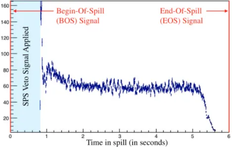
22.3.2 Beam Structure Study . . . 109

23 Results: Systematic Uncertainties, Summary, Figure of Merit 111

VI

Measurement of Drell-Yan Cross-Sections

113

24.2 Event Selection . . . 115

24.3 Additional Studies . . . 119

24.3.1 Period Compatibility . . . 119

24.3.2 Dimuon Data Yield . . . 119

24.3.3 Combinatorial Background Estimation . . . 121

24.3.4 Target Tomography and Beam Positioning . . . 122

25.2 Event Generation . . . 127

25.3 Spectrometer Acceptance . . . 130

25.3.1 Geometrical Acceptance . . . 130

25.3.2 Event Migration and Detector Inefficiencies . . . 131

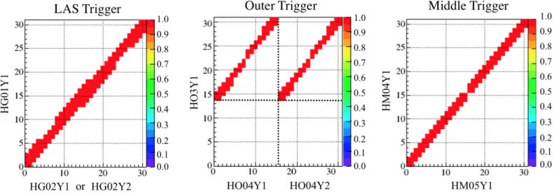
25.3.3 Trigger System Efficiency . . . 134

25.3.4 Overcorrection of the Beam Telescope Acceptance . . . 137

25.4 Multi-Dimensional Acceptance . . . 138

25.5 Model-Dependent Uncertainties . . . 141

26 Introduction to the Absolute Drell-Yan Cross-Sections 145 26.1 The Drell-Yan Cross-Section Per Nucleon . . . 145

26.2 Perturbative QCD Predictions at NNLO . . . 145

26.2.1 Parton Level Monte Carlo, DYNNLO . . . 145

26.2.2 Drell-Yan Predictions at COMPASS energy (√s = 18.90 GeV) . . . 146

26.3 Discussion on the Single Differential Cross-Sections dσ/dxF . . . 149

26.4 Summary of the Final Uncertainties . . . 150

27 Results: Extraction of the Drell-Yan 2015 Cross-Sections 151 27.1 Study of the Double Differential Drell-Yan Cross-Sections . . . 151

27.1.1 Comparison with E615 data and DYNNLO simulation . . . 151

27.1.2 Cross-Section d2_σ/d√_{τ dx} F in the COMPASS Kinematic Range . . . 155

27.1.3 Summary Table . . . 156

27.2 A-Dependence in Pion-Nucleus Interactions . . . 158

27.2.1 Evaluation of the α parameter . . . 158

27.2.2 Summary Table . . . 160

27.3 Drell-Yan Cross-Sections at High-qT . . . 161

27.3.1 Transverse Momentum Distributions . . . 161

27.3.2 The Kaplan Form: Ad-Hoc Fitting Function . . . 161

27.3.3 Studies as a function of xF, Mµµ, √ s . . . 162

27.3.4 Invariant Cross-Sections at High-qT, Ed3σ/d ⃗q3 . . . 164

27.3.5 Summary Table . . . 166

27.4 Invariant Double Drell-Yan Cross-Sections M2_d2_σ/dx 1dx2 . . . 168

27.4.1 Motivations . . . 168

27.4.2 Summary Table . . . 169

Conclusions and Future Prospects

171

Appendix

173

Résumé en Français

191

Introduction

A bit of history

It has been 100 years from now, in 1919, that Ernest Rutherford made the proof of the existence of the proton using nitrogen nuclei targeted with alpha particles. Initially denoted as a hydrogen atom, the accurate definition of the proton appeared in 1920. A decade later in 1932, James Chadwick discovered the neutron and both protons and neutrons were considered at that time as elementary particles.

Owning of the discovery of a large variety of other particles, such as muons in 1937 by Carl D. Anderson, or the π meson in 1947 by Cecil F. Powell, the classification of these particles have appeared to be a challenging task. The great physics quest, also known as a quest for symmetries, began to organize this particle zoo. As a successful example, particles such as the proton and the neutron were eventually classified among other particles (Fig. 1a), following the Eightfold Way model [1] proposed by Murray Gell-Mann and Yuval Ne’eman in 1961. In 1964, this hadron classification model successfully led to the prediction of the baryon Ω− (Fig. 1b) according to symmetry conservation. As an illustration, Fig. 1 shows the baryon octet and decuplet of the Eightfold Way model.

Figure 1: (a) Left: Baryon Octet JP ₌1

2

+

; (b) Right: Baryon Decuplet JP ₌3

2

+

Later in 1964, Murray Gell-Mann and Georges Zweig postulated the existence of elementary subatomic particles in two independent papers [2] [3], known nowadays as quarks. These quarks are consequently assumed to arrange themselves into hadron particles. The first evidence of an internal structure in nucleons was revealed in late 1960 at SLAC1 _{[4] using deep inelastic electron-nucleon scattering at high}

energy. In the early years, this model was composed of three quarks: the quark up and down, which compose neutrons and protons, and the strange quark (e.g., kaon).

Figure 2: Mass spectrum showing the existence of the J/Ψ and taken from [5]

The existence of charmed quarks was theorized first by Bjorken and Glashow in 1964 [6] and sup-ported by Glashow, Iliopoulos, Maiani in 1970, as a cure of the hadron weak interactions in the de-scription of the GIM mechanism [7].

Consequently, in 1974, the validity of the quark model was again strongly reinforced, when the discovery of the J/Ψ particle was confirmed at SLAC by Burton Richter et al. [8] and at BNL2 _{by Samuel Ting et al. [5]. This}

break-through discovery, as part of the November Rev-olution, confirmed the existence of the charm quark.

Following this epoch of great discoveries aiming to establish a Standard Model of particle physics, some natural questions arose, such as the origin of quantum numbers and their relation with the

intrinsic numbers of subatomic particles. Consequently later in 1987, the EMC3 _{collaboration measured}

a contribution of the quark spin to the total spin of the nucleon [9]. A possible decomposition of the nucleon spin into quark, gluon, and orbital contributions is proposed in Eq. 1 (spin sum rule), and illustrates the beginning of the proton spin puzzle.

1 2 = 1 2∆Σ(Q 2_{) + ∆G(Q}2_{) + L} q(Q2) + Lg(Q2) (1)

where ∆Σ, is the quark spin contribution to the nucleon spin ∆G, refers to the gluon spin contribution to the nucleon spin Lq/g, is the orbital momentum of the quark, gluons respectively

and Q2_{, is the energy scale related to the photon virtuality}

This example led to further investigations of the proton spin decomposition by several other experi-ments at CERN4_{, DESY}5_{, SLAC, JLAB}6_{, and RHIC}7_{. It has recently been established that quarks carry}

only 30%± 4% of the nucleon spin at Q2_{= 3 GeV}2_/c2_{. Additionally, ∆G was found as very close to zero}

[10] and the orbital momentum remains under study.

In 2005, the measurement of the non-zero Sivers function via Deep Inelastic Scattering (DIS) by HERMES [11] and COMPASS [12] raised the interest of the study of the Drell-Yan process by crossing

2_{Brookhaven National Laboratory (Upton, NY, USA)} 3_{European Muon Collaboration}

4_{European Organization for Nuclear Research (Meyrin, Switzerland)} 5_{Deutsches Elektronen-Synchrotron (Hamburg, Germany)}

6_{Thomas Jefferson National Accelerator Facility (Newport News, VA, USA)} 7_{Relativistic Heavy Ion Collider at BNL (Upton, NY, USA)}

symmetry with DIS. Indeed, the Drell-Yan process (q ¯q−→ ℓ−ℓ+_{at lowest order) is also an excellent tool}

to study the properties of the Quantum Chromodynamics (QCD) physics. Therefore, the measurement of the polarized single-spin asymmetries through Drell-Yan became a fundamental verification of TMD8

factorization in QCD [13].

Finally, Drell-Yan data offers valuable information about the partonic composition of the beam, but also information about cold nuclear matter effects in the target. Therefore, the evaluation of the Drell-Yan cross-section using COMPASS data might significantly contribute to a better knowledge of these topics.

Outline of this Ph.D. work

This Ph.D. work is decomposed into six chapters. The first chapter introduces the theoretical frame-work of the QCD theory and focuses on the Drell-Yan process. The interest in cross-section extraction will be then emphasized by summarizing the state-of-the-art of some Drell-Yan advanced analysis.

The second and third chapters refer to the hardware aspects of the COMPASS-II experiment. As the COMPASS-II spectrometer is a versatile apparatus, the second chapter highlights only the setup related to the Drell-Yan data taking. The third chapter provides further hardware information about the Straw detector, ST03, supported by the University of Illinois since 2014. Part of this Ph.D. work consisted of maintaining the ST03 detector from 2016 to 2018 in collaboration with the Joined Czech group from Prague.

The fourth chapter is mainly software related and includes an overview of the COMPASS reconstruc-tion software, the MC simulareconstruc-tion of the COMPASS apparatus, and the working principle of a new data production framework called ESCALADE to organize the large production of COMPASS data. During this work, a new petascale computing center was used for intensive computing jobs, such as track recon-structions of the COMPASS data or MC simulations.

Finally, the fifth and sixth chapters give the detailed methodology related to the extraction of the beam luminosity, the computation of the acceptance correction, and the Drell-Yan cross-section. The obtained results are eventually compared with the predictions of Drell-Yan cross-section and already published results.

Disclaimer

This manuscript is written in the light of the COMPASS analysis status of the Drell-Yan working group dated November 2019. The results presented in this Ph.D. thesis are a personal interpretation of the COMPASS 2015 data.

Chapter I

Internal Structure of Hadrons

1 Modern Theory of the Strong Interaction 6

1.1 The Parton Model . . . 6

1.2 Introduction to Quantum Chromodynamics (QCD) . . . 7

1.3 Color Confinement and Asymptotic Freedom . . . 8

1.4 The QCD improved Parton Model . . . 9

2 The Deep Inelastic Scattering 11 3 The Drell-Yan Annihilation Process 14 3.1 Introduction to the Drell-Yan Process . . . 14

3.2 General Expression of the Cross-Section . . . 17

3.3 Lorentz Invariant Cross-Sections . . . 18

3.4 Experimental Overview . . . 19

4 Theoretical Overview: State-of-the-Art 21 4.1 Drell-Yan Angular Distributions and Lam-Tung Relation . . . 21

4.2 Cold Nuclear Matter . . . 23

4.3 A-dependence of Muon Pair Production . . . 25

4.4 Soft-Gluon Resummation . . . 26

4.5 Parton Distribution Functions of the π− . . . 27

4.5.1 Experimental Overview . . . 27

4.5.2 Global Analysis of the Pion PDFs . . . 30

4.5.3 Available Pion PDF Extractions . . . 31

This chapter describes some theoretical aspects related to the theory of Quantum Chromodynamics and focuses on the study of the Drell-Yan process involving a π−beam. A state-of-the-art is also presented together with phenomenological aspects, where the COMPASS data might contribute.

1

| Modern Theory of the Strong Interaction

In analogy to the Van der Waals force, which binds atoms together to form molecules, the strong interaction binds quarks into nucleons. The strong force, known as one of the four fundamental forces in nature, has been described in the framework of Quantum Chromodynamics (QCD), in which quarks interact via gluons by exchanging color charges. At this time, QCD is widely accepted in the physics community as a pillar of the Standard Model (SM).

1.1 The Parton Model

In the early years, hadrons were assumed to be elementary particles. As an example, this assumption was reasonable in the low-energy limit described by the Rutherford scattering. However, the evidence of an internal structure was first raised from a series of electron-nucleon scattering experiments at SLAC starting in 1967 [14].

Indeed, at higher energy scale (Q ≫ ΛQCD) hadrons breaks up and reveals their composite nature

made of quarks, antiquarks, and gluons initially called partons by Richard Feynman. The parton model, proposed by Feynman in 1969, describes the internal structure of nucleons as the composition of partons. In the case of two colliding hadrons A and B, the corresponding cross-section follows the expression :

dσAB ≃ ∑ a,b ∫ 1 0 dx1fa/A(x1)× ∫ 1 0 dx2fb/B(x2)× dˆσab (1.1)

The labels a and b refer to partons in the nucleon A and B respectively. The density distribution fa/A(x1), also known as Parton Distribution Function (PDF), is the probability of finding a parton a,b

carrying a momentum fraction x1,2 in the corresponding nucleon. Eq. 1.1 highlights the independent

nature of the hard and the soft production mechanisms assumed by the factorization theorem [15, 16]. This theorem also ensures the universality of the measured PDF, regardless of the physics process involved. On the one hand, the hard-process, responsible for the short-range interactions, is described by the partonic cross-section dˆσab. On the other hand, the PDFs carry the soft information related to the

initial-state. Figure 1.1 shows an illustrative example of the interaction between u− ¯u quarks in a π−_p

interaction.

Figure 1.1: Illustration of the interaction between u−¯u quarks in a π−_{p collision, where u carries a fraction}

1.2

Introduction to Quantum Chromodynamics (QCD)

Near to the well-defined theory of Quantum Electrodynamics (QED), the Quantum Chromodynamics (QCD) is also known as a gauge theory. In its framework, the QED theory is described using the U(1) local gauge, while the more complex QCD theory is specified using a non-abelian SU(3) symmetry group. This QCD gauge theory involves eight massless gluons corresponding to the eight generators of the SU(3) symmetry. The Lagrangian of the free quark motion is expressed as follows:

Lfree= 6 ∑ q=1 ¯ ψi (q) (i /∂− mq)ψ (q) j (1.2)

In Eq. 1.2, q refers to the six quark flavors (Nf = 6) subjected to the strong interaction. ψ(q)

corresponds to the Dirac spinor of the quark q and mq the mass of the quarks. i and j are color indices

in the range{1..Nc} with the number of color charges, Nc= 3. QCD requires that the Lagrangian must

be invariant under the local SU(3) gauge transformation U (x): ψ(x)−→ ψ′(x) = U (x)ψ(x) = exp [ igs⃗α(x)· ˆT ] ψ(x) where _{T =}ˆ _{Ta_{} =} { 1 2λ a }

are the eight generators of SU(3) related to

Gell-Mann matrices, λi, with a the color index∈ {1..8}

⃗

α(x) ={αa(x)} are eight functions of the space-time coordinates x (rotation angles). gs=

√

4παs refers to the QCD coupling variable

U (x) is a unitary 3×3 matrix acting on the color state ψ(x)

Under this local gauge transformation, Eq. 1.2 becomes: iγµ_(∂

µ+ igs(∂µ⃗α(x)). ˆT− mq)ψ(q) = 0. In

this equation, the terms ∂µαa(x) are identified as eight gauge fields Gaµ. Moreover, the conservation of the

local SU(3) symmetry requires the introduction of the covariant derivative term ∂µ→ Dµ= ∂µ+igsGaµTa

to ensure gauge invariance.

The dynamics of the gluon field is described by a Lagrangian kinematic term in Eq. 1.3. Moreover, the non-commutative nature of the SU(3) group led to the introduction of an additional term in the field-strength tensor: Gi µν = ∂µGiν− ∂νGµi − gsfijkGjµGkν Lkin=− 1 4G a µνG µν a (1.3)

Finally, the gauge-invariant QCD Lagrangian is given by the Eq. 1.4. The first line of this Lagrangian equation can be intuitively decomposed into four types of Feynman diagrams, as shown in Fig. 1.2.

LQCD = Nf ∑ q=1 ¯ ψ(q)(i /D− mq)ψ(q)− 1 4G a µνG µν a = q ¯q + G2 | {z } (a) + g_{| {z }}sq ¯qG (b) + gsG3+ gs2G 4 | {z } (c)+(d) (1.4)

Figure 1.2: (a) Quark-gluon propagators; (b) Quark-Gluon coupling; (c,d) Self-interacting gauge bosons The first case (a) corresponds to the propagators of quarks and gluons. The second term (b) describes the interaction between quarks and gluons. Finally, the last terms (c,d) are specific to the SU(3) local gauge-invariant theory and describes the self-interaction of the gluons as triple and quartic vertices.

1.3 Color Confinement and Asymptotic Freedom

In the QCD theory, the fundamental parameters are the quark masses mq and the gs quantity. The

gs parameter can also be expressed as the coupling strength αs(Q2) = g2s(Q2)/4π, where Q refers to the

hard scale of a process. The origin of αsevolution, as a function of Q2, comes from the scale dependence

of the gauge theory in QCD. Eq. 1.5 arises from the renormalization theory: αs(Q2) = αs(µ2) 1 + B αs(µ2) ln ( Q2 µ2 ), with B = (11Nc− 2Nf) 12π (1.5)

In the regime of non-perturbative QCD, quarks are confined into a color-neutral hadron. This effect is known as the confinement phenomenon. Oppositely, in the perturbative QCD (pQCD) at large Q2_,

quarks behave like quasi-free particles. This second phenomenon described by Politzer [17], Gross, and Wilczek [18], is known as asymptotic freedom. A fundamental parameter ΛQCD, in the order of few

hundred MeV, defines the separation between the perturbative and non-perturbative regime.

As QCD is a gauge field theory, the effective strength of the interaction αs(µ2) at the vertex point is

determined by a renormalization factor µ. In the QED theory, this factor is chosen to avoid divergence of loop diagrams at large scale. Indeed, the electromagnetic coupling αQED becomes stronger when Q2

increases: it often refers to the charge screening of QED in the literature. At low energy scale, the coupling constant matches the measured fine structure constant: α(µ2_{≃ 0) =} 1

4πε0

e2 0

ℏc.

By analogy to QED, the renormalization factor µ of the QCD theory is chosen to avoid divergences of the theory owning for example gluon self-interactions. In the perturbative regime (µ2 _{≫ Λ}2

QCD), a

solution for Eq. 1.5 is obtained in the 1-loop approximation from the renormalization group equations (RGE): αs(Q2≃ µ2) = 1 B ln ( Q2 ΛQCD

), with ΛQCD≃ few 100 MeV (1.6)

For a given physics process, the strength of the coupling is expressed as a function of the hard scale Q, such that Q2 _{≃ µ}2_{. Short-distance interactions, at a high momentum (Q ≫ Λ}

QCD), are well

perturbative regime through different channels. On the opposite, the soft part, related to long-distance interactions, has a non-perturbative origin, cannot be described analytically, and consequently requires a phenomenological approach.

Figure 1.3: Evolution of the strong coupling constant αs as a function of Q [19]

1.4

The QCD improved Parton Model

In the limit of an experimental measurement, the asymptotic freedom (Q2_{→ +∞) will no longer be}

assumed and leads to the introduction of a finite energy Q0, such that Q2→ Q20. It results in a QCD gluon

field in the description of the parton model. Therefore, in addition to the initial renormalization factor µ, a second arbitrary scaling parameter µF is introduced to renormalize the collinear gluon contribution.

In the following, µF is chosen as µF ≃ µ. Fig. 1.4 illustrates the screening of the gluon radiation in the

initial-state when a virtual photon interacts below the threshold Q2_{= Q}2 0.

Figure 1.4: Illustration of the gluon radiation, this effect is of the order of O(αsln(Q2))

Consequently, the following three processes involving gluons, allowed by the QCD Lagrangian, arise : gluon radiation (q → qg), gluon splitting (g → gg), and quark-antiquark pair production (g → q¯q). The

introduction of these corrective terms leads to a logarithmic dependence in Q2_{of the physical observables.}

The scale dependence of the PDFs1_{and FFs}2_{is described by the DGLAP}3_{equations [20].}

dqi(x, Q2) dln(Q2₎ = αs(Q2) 2π ∫ 1 x ( qi(z, Q2)Pqq (_x z ) + g(z, Q2)Pqg (_x z ) )_dz z dg(x, Q2₎ dln(Q2₎ = αs(Q2) 2π ∫ 1 x ( ∑ i qi(z, Q2)Pgq (_x z ) + g(z, Q2)Pgg (_x z ))_dz z (1.7)

At the lowest order, these equations are driven by the four splitting functions : Pqq,Pqg,Pgq,Pgg.

These functions, Pji(x/z), can be interpreted as a density probability of turning a parton i of momentum

fraction z into a parton j carrying a momentum fraction x of the initial momentum.

Figure 1.5: Feynman diagrams for lowest order splitting functions Pqq,Pqg,Pgq,Pgg.

Finally, Fig. 1.6 illustrates the Q2_{evolution introduced by the DGLAP equations for quark and gluon}

PDFs. This figure shows PDFs at two different energy scales. This results have been obtained from the quark and gluon PDFs extracted by the CT14 collaboration at NNLO4_.

Figure 1.6: Comparison of the distribution xf (x) from CT14nnlo (C.I = 90%) at Q2 _{= 10 GeV}2 _(left)

and Q2_{= 10}5_GeV2_(right).

1_{Parton Distribution Functions} 2_{Fragmentation Functions}

3_{Dokshitzer-Gribov-Lipatov-Altarelli-Parisi} 4_{Next-To-Next Leading Order}

2

| The Deep Inelastic Scattering

Deep Inelastic Scattering (DIS) has played a fundamental role in determining the composite nature of the proton and the existence of quarks. Using a probe, such as e−, that interacts in a well understood electromagnetic interaction, makes it a privileged channel for such studies. In DIS, only the outgoing lepton is measured. The hard scale Q is defined as the negative four-momentum squared of the virtual photon. At a large Q2_{scale, the DIS is an extension of the Rutherford scattering, where the lepton knocks}

a quark out of the nucleon. It is interesting to note that DIS is a highly inelastic process as far as the target nucleon is concerned. In the quark-parton model, DIS can be considered as an elastic scattering between the electron and the quark.

Figure 2.1: Typical behavior of the electron–proton differential cross section as a function of the invariant hadron mass W in the final-state. It illustrates the transition between elastic scattering, quasi-elastic (or nucleon resonances) and deep inelastic scattering [21]

At the Born level, DIS is a process described by the exchange of a virtual photon γ∗ (or a weak boson Z0_{for collider energies) between an incoming lepton beam scattering off a nucleon target, as illustrated}

in Fig. 2.2.

ℓ(k) + N (P )−→ ℓ(k′) + X

The momentum of the incoming and outgoing leptons are measured. The hadronic final-state X consists of many particles. This process is called inclusive when the hadronic final-state is not measured. The semi-inclusive DIS refers to the case where at least one hadron is measured in the final-state.

Kinematic of DIS. Two independent variables, often chosen as (x, Q2_{), are sufficient to describe the}

inclusive DIS process. However, other kinematical combinations would also be possible. The kinematics of the DIS process is obtained from the four-momentum of the lepton k, and k’, in the initial and final-state. In the context of a fixed-target experiment, the target four-momentum vector is P = (M,⃗0). The Bjorken-x scaling variable is interpreted as the nucleon momentum fraction carried by the quark, and the hard scale of the reaction Q2 _{is given by the negative four-momentum squared of the exchanged virtual}

photon. The center-of-mass energy of the photon-nucleon system is denoted W = (P + q)2_{, and the DIS}

kinematic region is defined in the limit of W ≫ M2_{and Q}2_{> 1.}

     Q2 _{= −q}2_{=−(k − k}′₎2 x = Q 2 2P.q (2.1)

Other variables, such as the beam momentum fraction carried by the virtual photon denoted y or the photon energy ν in the target rest frame, are widely used in the literature and defined as follows.

y = P.q

P.k ν =

P.q

M (2.2)

Quark Parton Model. The QPM1 _{is defined in the infinite momentum frame. In that frame, the}

nucleon has a very large momentum such that the transverse component of partons is neglected. The expression of the unpolarized differential cross-section for DIS, Eq. 2.3 is derived from the contraction of the leptonic tensor Lµν _{and hadronic tensor W}

µν. In the QPM, the hadronic tensor is expressed as the

incoherent sum of the interactions with each parton. d2_σ dxdQ2 = 4πα2 Q4 [ (1− y)F2(x, Q 2₎ x + y 2_F 1(x, Q2) ] (2.3) In the late 60s, two features related to the two spin-independent structure functions F1 and F2 were

found at SLAC. The first one is known as Bjorken-scaling, where F1(x, Q2) and F2(x, Q2) were found to be

almost Q2_{independent, indicative of the point-like nature of quarks. The two spin-independent structure}

functions, F1(x) and F2(x), interpreted as the number density of quarks and the quark momentum

distribution functions respectively, are given in the QPM as:          F1(x) = 1 2 ∑ q e2_q[q(x) + ¯q(x)] F2(x) = x ∑ q e2_q[q(x) + ¯q(x)] (2.4)

where q(x) refers to the PDF of the interacting quark eq corresponds to the quark charge

The second feature observed is the relation between F1(x) and F2(x), also known as the Callan-Gross

relation [22]. This relation reflects the spin-½ nature of the quarks.

F2(x) = 2xF1(x) (2.5)

Scaling Violation. The world data of the proton structure function Fp

2 is shown in Fig. 2.3. Over

this broad coverage in x, this plot reveals the scaling violation of the Q2 _{variable and the necessity to}

account for additional QCD corrections in the parton model. This correction is interpreted as the gluon contribution to the DIS cross-section.

Figure 2.3: The world data of the proton structure function Fp

2 as a function of Q2 for different bins of

3

| The Drell-Yan Annihilation Process

3.1

Introduction to the Drell-Yan Process

Figure 3.1: Differential cross-section as a function of the dimuon mass mµµin high-energy hadron collisions

at Eproton = 28.5 GeV [24]

The first experiment measuring hadro-production of lepton pairs took place at AGS1_in

Brookhaven in 1968 and was reported few years later in November 1970. Christenson, Hicks, Lederman, Limon, Pope and Zavatini [24] mea-sured the reaction products of the following col-lision at 28.5 GeV beam energy :

p + U → µ−+ µ++ X

The remnant term X was not measured and the detection of penetrating muons is often preferred for experimental reasons compared to electrons. In Fig. 3.1, the dilepton cross-section, in the range 1 < Mµµ/(GeV/c2) < 6.7, was later

de-scribed as the combination of charmonium reso-nances (J/Ψ and Ψ′) production around 3 GeV and 4 GeV and a continuous spectrum.

In August 1970, Sidney Drell and Tung-Mow Yan published a paper [25], which identified the mech-anism responsible for this continuum and proposed the production model, which now bears their name. The Drell-Yan mechanism, describing the high mass lepton pair production in inelastic collisions, is illustrated as shown in Fig. 3.2.

Figure 3.2: Feynman diagram of the Drell-Yan process, producing a lepton pair ℓ¯ℓ from the annihilation of a quark-antiquark pair q ¯q. The X terms are the remnant hadrons resulting from the inelastic interaction between the hadrons H1and H2.

A general expression of the Drell-Yan process involves a quark-antiquark pair q ¯q originating from two colliding hadrons H1 and H2. These latter interact as follows:

H1(P1) + H2(P2, ⃗S)−→ q(p1) + ¯q(p2) + X−→ ℓ−(pℓ−) + ℓ+(pℓ+) + X

At leading order, the quark-antiquark pair q ¯q annihilates into a virtual photon γ∗(q) or the weak boson Z0 _{(Fig. 3.3). The mediating boson turns into a lepton pair ℓ¯ℓ measured by an experimental}

apparatus. The outgoing remnant hadrons X are not measured. P1 and P2 are the beam, and the

target energy-momentum vectors, with S defined as the spin vector in the target rest frame (Fig. 3.4). The center-of-mass energy √s is related to the two hadronic vectors, as shown in Eq. 3.1. The four-momentum vector of the mediating particle is denoted q = pℓ− + pℓ+, where p_ℓ± refer to the leptonic four-momentum vectors. Moreover, the hard scale Q is given by the measured mass M of the dilepton.

Figure 3.3: Feynman diagram at leading order of the Drell-Yan reaction q ¯q→ ℓ−ℓ+

{

Q2 _{= q}2_{= M}2

s = (P1+ P2)2

(3.1)

Quark four-momenta, p1and p2, are related to hadron four-momentum via the Bjorken scaling variable

for each hadron, denoted x1 and x2, as shown in Eq. 3.2. Other dimensionless variables, namely xF and

τ are deduced from x1 and x2, as xF = x1− x2 and τ = M2/s.

   p1 = x1P1 p2 = x2P2 with x1,2 defined as x1,2= Q2 2P1,2.q (3.2)

Target Rest Frame. This reference frame, Fig. 3.4, is defined by the unit vector ˆz aligned with respect to the beam momentum. The ˆx unit vector is along the transverse component qT of the virtual photon.

Finally, the last unit vector is deduced as ˆy = ˆz× ˆx. In this reference frame the main vectors are defined

as follows: _             P1 = (E1, 0, 0, P1z) P2 = (Mp, 0, 0, 0) q = (Eγ, qT, 0, qL) S = (0, STcos ϕS, STsin ϕS, SL) (3.3)

Collins-Soper (CS). This frame is defined in the rest frame of the dilepton as shown in Fig. 3.5. The ˆ

z is aligned with respect to the bisector of ⃗Pa and− ⃗Pb hadron momenta. The ˆy axis is perpendicular to

the hadron plane formed by ˆPa and ˆPb, while ˆx axis lies on the hadron plane. In this frame, the leptonic

four-momenta are :    pℓ− = q

2(1, sin θCScos φCS, sin θCScos φCS, cos θCS) pℓ+ =

q

2(1, − sin θCScos φCS, − sin θCScos φCS, − cos θCS)

(3.4)

Figure 3.5: Definition of polar and azimuthal angles θCS and ϕCS of the lepton ℓ− momentum in the

Collins–Soper frame [26]

Degree of freedom of the Drell-Yan Process. The Drell-Yan process is often described by the two parameters (xF, M), but the kinematic of this process can also be expressed in terms of other variables,

such as (x1,x2). From an experimental point of view, the measurement requires eight parameters, namely

the two four-momentum vectors of the measured leptons. These degrees of freedom can be reduced to six free parameters using the mass constraints for the two leptons. Moreover, different systems of equations can be used to describe the Drell-Yan process. However, a convenient system of six parameters might involve the following variables: (M, xF, qT, ϕLAB, cos θCS, φCS). Additionally, for unpolarized Drell-Yan,

the azimuthal symmetry reduces the degree of freedom to five variables (no ϕLABdependence).

Correction diagrams. Additional diagrams are accounted at next-to-leading order and involve gluon interactions. These diagrams contribute to energy loss effects and the production of a large transverse momentum qT. Fig. 3.6(a) shows the vertex correction diagram. Moreover, Fig. 3.6(b,c) involve the

emission of a gluon, and together with Fig. 3.6(a) represent the annihilation diagrams. The Compton diagrams involving a gluon in the initial-state are shown Fig. 3.6(d,e) .

3.2

General Expression of the Cross-Section

The factorization theorem allows decomposing the hadronic cross-section into the hard process and the soft part. Consequently, these terms are expressed independently in the following.

Hard cross-section. The underlying process behind the hadro-production of lepton pairs is described by the q ¯q annihilation via the exchange of a virtual photon γ∗, as shown in Fig. 3.7.

Figure 3.7: Feynman diagram at leading order of the partonic Drell-Yan reaction q ¯q→ ℓ−ℓ+

The Feynman rules of this diagram gives the following transition matrix element : − iM =[u¯q(p2)(ieqeγµ)vq(p1) ]gµν q2 [ ¯ uℓ(pℓ+)(ieγν)vℓ(pℓ−) ] (3.5)

The expression of the annihilation cross-section, e+_e− _{→ ℓ}+_ℓ−_{, in QED is similar to the expression of}

the Drell-Yan cross-section in the QCD description. In the interaction between q ¯q→ ℓ+_ℓ−_{, an additional}

term Nc is introduced as a result of the color conservation of the QCD theory. In the annihilation

process, only the non-zero matrix elements related to r¯r, g¯g, b¯b color factors are possible. Consequently, the unpolarized cross-section is obtained by averaging over spin and color states as follows:

⟨|M |⟩2₌ 1 9 ∑ color  1 4 ∑ spin | − iM |2   = e4e2q Nc (1 + cos2θ) (3.6)

As a simple example, the expression of the differential cross-section q ¯q→ ℓ¯ℓ is given as follows. dσ

dΩ= 1

64π2_ˆs⟨|M |⟩

2 _(3.7)

where s = (pˆ 1+ p2)2≃ x1x2s refers to the center-of-mass energy of the q ¯q system.

Consequently, the known expression of the total cross-section ˆσ(q ¯q→ ℓ¯ℓ) at the Born level is retrieved as shown in Eq. 3.8 by integrating over the full solid angle (4π steradians), and by neglecting the proton mass (p2 1= p22≃ 0). ˆ σ(q ¯q→ ℓ¯ℓ) = e 2 q Nc 4πα2 3ˆs (3.8)

where α = e2_{/4π is the fine structure constant}

eq is the quark charge

Soft non-perturbative contribution. In addition to the hard cross-section, a non-perturbative con-tribution, related to the definition of parton distribution functions of hadrons in Fig. 3.7, arises in the expression of the double differential cross-section as a function of dx1 and dx2. The quark q1, originating

from a beam particle, interacts with the antiquark ¯q2 of a target nucleon. By symmetry, the two quark

PDF combinations, q1(x1)¯q2(x2) and ¯q1(x1)q2(x2), are possible and lead to the following differential form.

d2σ =[q1(x1)¯q2(x2) + ¯q1(x1)q2(x2)

] ˆ

σ(q ¯q→ ℓ¯ℓ)dx1dx2 (3.9)

As suggested by Eq. 1.1, the Drell-Yan differential cross-section can be expressed in terms of the two scaling variables (x1,x2) and the structure function F (x1, x2) related to the quark PDFs, by summing

over all quark flavors. d2_σ dx1dx2 = ( 4πα2 9M2 ) ∑ q e2_q[q1(x1)¯q2(x2) + ¯q1(x1)q2(x2) ] = 1 M2F (x1, x2) (3.10)

3.3 Lorentz Invariant Cross-Sections

The invariance of the cross-section under Lorentz transformation is an advantage to facilitate com-parisons with other measurements. As an example, Eq. 3.10 may be written in terms of the Lorentz invariant function F (x1, x2) :

M2 d

2_σ

dx1dx2

= F (x1, x2) (3.11)

Moreover, this invariant cross-section, Eq. 3.11, can also be expressed in terms of (Mµµ,xF) using

the change of variable theorem. This theorem allows to write down the following integral relation, using G :(x1, x2 ) 7−→(M2= sx1x2, xF = x1− x2 ) ∫∫ σ(M, xF)dxFdM = ∫∫ σ(G(x1, x2))detJG(x1, x2)dx1dx2 =⇒ M3 d 2_σ dM dxF = 2x1x2 (x1+ x2) × F (x1, x2) (3.12)

The latter invariant cross-sections (Eq. 3.12 and Eq. 3.11) are both used under an integrated trans-verse momentum of the dimuon qT. However, the invariant triple differential cross-section (Eq. 3.13) is

expressed as a function of xF, but carries also the information of the transverse momentum qT. Along the

same line of variable change (F being analog to the G application) and by assuming azimuthal symmetry, the triple differential cross-section can be expressed, as follows:

∫

σ(⃗q)dq3= ∫∫∫

σ(F (qL, qT, ϕLAB))detJF(qL, qT, ϕLAB)dqLdqTdϕLAB

=⇒ Ed 3_σ d ⃗q3 = 4E √ s× d3σ dxFdq2TdϕLAB ϕLAB −−−−→_sym. Ed 3_σ d ⃗q3 = 2E π√s × d2σ dxFdqT2 (3.13)

3.4

Experimental Overview

Following the first report about dimuon production at AGS, various experiments measured the dilepton production over the years using either proton-proton, proton-nucleus, or pion-nucleus collisions (Tab. 3.1). This non-exhaustive list highlights the worldwide interest to study and understand the dimuon spectrum. This interest culminated in 1983 when the UA1 and UA2 experiments at CERN discovered the W, Z bosons using the Drell-Yan process in ¯p− p collision.

Table 3.1: Summary table of some muon pair production experiments [27]

Reactions Experiments Targets √s [GeV] δsys. (%) References

pp−→ e+_e−_{+ X R108 H}

2 62.4 12% Angelis et al. (1979) [28]

R808 H2 53; 64 50% Kourkoumelis et al. (1979) [29]

pp−→ µ+_µ−_{+ X R209 H}

2 44; 62 15% Antreasyan et al. (1981) [30]

pA−→ µ+_µ−_{+ X E288 Pt 19.4; 23.7; 27.4 ≳ 25% Ito et al. (1981) [31]}

E325 Cu 19.4; 23.7; 27.4 N/A Antreasyan et al. (1979) [32] E444 C,Cu,W 20.5 15% Anderson et al. (1979) [33] E439 W 27.4 11% Smith et al. (1981) [34]

NA3 Pt 27.4 12% Badier et al. (1985) [35] E772 H2 38.7 N/A Alde et al. (1990) [36]

E605 Cu 38.7 ≃ 18% Moreno et al. (1991) [37] ¯

pA−→ e+_e−_{+ X UA1 – – – –}

UA2 H2 630 20% Alitti et al. (1992) [38]

¯

pA−→ µ+_µ−_{+ X E537 W 15.3 5%-13% Anassontzis et al. (1988) [39]}

π±A−→ µ+_µ−_{+ X E326 W 20.5 15% Greenlee et al. (1985) [40]}

E444 C,Cu,W 20.5 15% Anderson et al. (1979) [33] WA11 Be 16.8; 18.1 20% Barate et al. (1979) [41] WA39 W 8.6 – Corden et al. (1980) [42]

NA3 Pt 16.8; 18.4; 22.9 12%-23% Badier et al. (1983) [43] NA10 W 19.1; 23.2 ≃ 10% Betev et al. (1985) [44]

E537 W 15.3 5%-13% Anassontzis et al. (1988) [39] E615 W 21.7 16% Conway et al. (1989) [45]

The NA10 and E615 experiments are of particular interest in comparison to the COMPASS Drell-Yan measurement on tungsten in 2015. Indeed, these experiments measured muon pairs originating from the interaction between an incoming π− and a tungsten target at similar center-of-mass energies, √

s = 19.07 GeV for NA10 [44] and √s = 21.74 GeV for E615 [45], compared to the COMPASS center-of-mass energy at √s = 19.89 GeV. The integrated cross-section and the corresponding K-factors are summarized in Tab. 3.2.

Table 3.2: K-factor obtained for some π−A−→ µ+_µ−_{X reactions [27]}

Experiment Reaction √s [GeV] Integrated σ0 [nb] Prediction NLO K-factor

NA10 (1985) π−W −→ µ+µ− 19.07 0.0803 0.0625 1.286± 0.005 E615 (1989) π−W −→ µ+_µ− _{21.74 0.1916 0.1801 1.064± 0.011}

The K-factor is conventionally defined as the ratio between the observed experimental cross-section and a theoretical prediction (either LO, NLO, or NNLO). This factor was historically used to illustrate the effect of higher-order corrections. In Tab. 3.2, the K-factor is computed using a theoretical prediction at NLO. The NLO calculation is parametrized using SMRS⊗MRS PDF sets [27] for the pion and the nucleon PDF, respectively.

Finally, results of the proton-induced Drell-Yan productions from NA3 [46] (triangles) at 400 GeV/c, E605 [37] (squares) at 800 GeV/c, and E772 [47] (circles) at 800 GeV/c is shown in Fig. 3.8. The parton model scaling properties is illustrated in this figure as in bins of xF. The absolute lines are computed at

NLO accuracy for p + d collisions at 800 GeV/c using the CTEQ4M structure functions [48].

Figure 3.8: Proton-induced Drell-Yan production from various fixed target experiments. This picture is taken from [49]

4

| Theoretical Overview: State-of-the-Art

An overview of some recent theoretical studies related to the Drell-Yan process is shown in this section. It aims to introduce some existing interpretations resulting from the analysis of past experiments and to highlight the motivations of extracting Drell-Yan cross-sections from the COMPASS data.

4.1 Drell-Yan Angular Distributions and Lam-Tung Relation

In the CS1 _{frame, Fig. 4.1, the angular differential cross-section of the lepton ℓ− for unpolarized}

Drell-Yan is expressed as a function of the three (λ, µ, ν) coefficients : 1 σ0 dσ dΩ= 3 4π 1 λ + 3 (

1 + λ cos2θ + µ sin 2θ cos Φ +ν 2 sin

2_{θ cos 2Φ})

where (θ, ϕ) denote the polar and azimuthal angle of the lepton ℓ− in the CS frame. (λ, µ, ν) are the three unpolarized Drell-Yan angular coefficients

σ0 is the angular integrated Drell-Yan cross-section.

Figure 4.1: Definition of the Collins–Soper frame [26]

At the Born level, considering the collinear hypothesis, the partonic interaction q ¯q → ℓ¯ℓ does not account for soft gluon exchanges or any QCD related processes. Consequently, the contribution of the primordial kT is neglected. In this naive model, the well known q ¯q annihilation cross-section Eq.4.1 is

retrieved, as the three asymmetry coefficients (λ, µ, ν) are expected to be equal to (1,0,0). 1 σ0 dσ dΩ= 3 16π ( 1 + cos2θ ) (4.1) The introduction of the gluon emissions results in a transverse momentum of the dilepton and leads to a modification of the unpolarized angular coefficients : (λ, µ, ν)̸= (1, 0, 0). These coefficients are expected to largely satisfy the Lam-Tung relation [50], Eq. 4.2 :

λ + 2ν = 1 (4.2)

This relation is analogous to the Callan-Gross relation and originates from the spin-½ nature of quarks. This relation was not expected to be sensitive to QCD corrections, unlike the Callan-Gross relation. The first measurements of Drell-Yan angular distributions were performed by the NA10 collab-oration [51] (1986) and the E615 collabcollab-oration [45] (1989) using a π+ _{beam over W target at 194 GeV/c}

and 252 GeV/c respectively. More recently, the E866 collaboration [52, 53] (2007) measured the distri-butions with a proton beam on a deuterium target at 800 GeV/c. This result is shown in Fig. 4.2. A sizable dependence was observed as a function of qT, and the violation of the Lam-Tung relation by E615

could not be explained by perturbative QCD corrections. Consequently, few years later , Boer suggested in 1998 [54] a possible contribution from a non-perturbative QCD effect might arise in the convolution of two unpolarized TMD PDFs : ν ∝ hq⊥

1 (p)⊗ h

q⊥

1 (π−).

Figure 4.2: Measurement of the λ, µ, ν coefficients in CS frame as a function of qT and evaluation of the

Lam-Tung relation carried out by the E866, NA10 and E615 collaborations [55].

In 2011 and 2015, respectively CDF and CMS experiments published new results in their respec-tive papers [56, 57]. The CDF collaboration seems to be in good agreement with the Lam-Tung rela-tion, while CMS observed a clear violation. These new measurements raised the interest of various theoretical groups to determine whether this vio-lation can be attributed to perturbative or non-perturbative QCD effect. As an example, the interpretation of the angular distributions of Z-boson production [55] brought new perspectives in the explanation of the Lam-Tung violation. Fig. 4.3 shows a comparison of CMS and CDF data with pure qG and q ¯q productions as a function of qT. This figure highlight the dependence of the

λ and ν parameters as a function of a mixture of 72.5% q ¯q and 27.5% qG respectively. Although a lot of efforts were involved in the understanding of the Lam-Tung violation, this relation remains under discussion and the COMPASS data might also provide valuable new insight.

4.2

Cold Nuclear Matter

The modification of the measured cross-section per nucleon on a heavy nucleus compared to a light nucleus was observed for the first time by the EMC2 _{collaboration in 1983 [58]. This effect, known as}

the EMC effect, has been extensively studied over the last 30 years. However, there is still no model at this time, which fully explains the initial observation. Nuclear dependences can be summarized into the three following items:

• EMC Effect, which is described by a modification of quark and gluon distributions (PDF) in bounded nucleons by a nuclear environment (1983). This effect is a function of the Bjorken-x of the target, as illustrated in Fig. 4.5.

• Energy Loss Effect, which describes the energy loss of quarks in the hadron beam while going across the nuclear target, as illustrated by Fig. 4.4a. This effect can be studied using either the Bjorken-x of the beam or xF. As an example, this figure shows a decrease of the nuclear corrective

factor at large xF due to the energy loss of the quarks in the initial-state, as predicted by the

BDMPS formalism [59].

• Cronin Effect, which describes the nuclear enhancement of high-pT hadrons due to multiple

interactions in nuclear matter, as illustrated Fig. 4.4b in terms of pT.

Figure 4.4: (a) Left: Prediction of the energy loss of the quarks in the initial-state [60] at COMPASS energy, using the BDMPS formalism; (b) Right: Illustration of the Cronin effect as a function of the pT

distribution visible in the ratio plot between heavy and light targets [61].

In Fig. 4.5, the combined data of the cross-section ratio from HERMES, SLAC-E139, and JLAB-E03103, highlight in a wide x range the nuclear dependence of the cross-section. It illustrates the Bjorken-x dependence of the ratio of cross-section, which is related to the structure-function in the measurement of the scattered electron via deep-inelastic scattering.

Figure 4.5: The ratio σC(N )/σD as a function of x from HERMES [62], SLAC-E139 [63], and

JLAB-E03103 [64]. (Adapted from [65])

The ratio σC(N )/σD in Fig. 4.5 can be subdivided into four regions as the following:

• The shadowing region (0 < x < x1 = 0.06); This region shows a cross-section ratio smaller than

1. The nuclear shadowing and anti-shadowing have a similar origin. These effects are produced by the coherence of quark-quark multiple scattering nuclear processes [66]. In addition, a destructive quantum-mechanical interference of the amplitude is responsible for the nuclear suppression at x < 0.06 [67].

• The anti-shadowing region (x1< x < x2= 0.30); In this region, the cross-section ratio is above 1.

• The valence-quark depletion region (x2 < x < x3= 0.8); This region shows a nuclear suppression

up to 10% as a function of x, also known as EMC effect. In this region, valence-quark distributions contribute more as x increases. At the highest x, the sea-quark is negligible.

• The Fermi motion region (x3 < x < 1); This region shows a rapid increase of the ratio as x

4.3

A-dependence of Muon Pair Production

In the Drell-Yan process, the incoherent nature of the quark-antiquark annihilation leads to an ex-pected linear dependence of the cross-section as a function of the atomic mass A. Consequently, the nuclear dependence of the cross-section per nuclei was historically [31, 43] parametrized using a power law as a function of the atomic mass A and an α parameter, such that :

σ(πA) = σA(πN )× Aα, where N refers to the nucleon [31] (4.3)

Along this line, α is expected to be 2/3 for the hadronic section, and close to 1 for Drell-Yan cross-section. The latter values are empirical estimations and the dependence as a function of the kinematics is not well known. This α parameter can be obtained from the measurement between cross-sections, σA1

and σA2, of two nuclei A1and A2respectively (A1 < A2) (Eq. 4.4) :

α (A2/A1) = ln ( σA2 σA1 ) / ln ( A2 A1 ) (4.4) Various experiments have measured the α parameter presented in Eq. 4.4. As an example, an evalu-ation of the α parameter by Ito et al [31] at Fermilab in the 80’s was performed using a proton beam at 400 GeV/c on both Pt and Be targets between 5 < M/(GeV/c2_{) < 11. The value of α as a function of the}

dimuon mass Mµµ and the pT distribution is shown in Fig. 4.6. Another evaluation of the α value was

performed using the NA10 data, π−over W (and D2) in the range 4.10 < M/(GeV/c2) < 11.79. Finally,

the NA3 collaboration also published a ratio between H2 and Pt targets [43]. Some known values of α

are summarized as follows :                   

αIto = 1.007± 0.018 (stat.) ± 0.028 (sys.)

αNA10 = 0.998± 0.006 (stat.) ± 0.013 (sys.) [68]

αNA3 = 1.03± 0.03 (π± on Pt [43]/H2)

αCFS = 1.02± 0.2 (p on Pt/Cu/Be [69])

αCIP = 1.12± 0.05 (π− on Pt/Cu/Be [70])

(4.5)

Figure 4.6: Values of α obtained from ratios of cross-sections σPt/σBeusing a proton beam at 400 GeV/c

from Ito et al. [31]. There is an additional 0.028 systematic uncertainty to include in the estimation of α at all masses and momentum.

4.4

Soft-Gluon Resummation

The detailed modeling and the interpretation of soft-gluon resummation are beyond the scope of this thesis but still require some introduction. As an example, refined interpretations of the Drell-Yan cross-sections were already intensively discussed in [71].

In the context of QCD theory, the soft-gluon radiation refers to the emission of gluon at very low energy. Below the energy threshold giving access to the final-state, the gluon emission originating either from quarks or gluons themselves is known as soft-gluon radiation. Soft-gluon radiations are induced by multiple scattering interactions in a nuclear medium and are modeled as a series of gluon interactions carrying small fraction ξk of energy, as illustrated in Fig. 4.7. The impact of soft-gluon resummation in

the description of the Drell-Yan process is significant due to the presence of quarks in the initial-state.

Figure 4.7: Illustration of the next-to-leading order soft gluon radiations

At the opposite of UV divergences (asymptotic freedom), a series of low energy interactions give rise to IR singularities. This IR divergences are a direct consequence of the massless nature of gluons. In other terms, some QCD correction diagrams of the soft-gluon radiations present divergent loop diagrams, which have to cancel because measured quantities are always finite. Consequently, a regularization is applied to the expression of the cross-section, which is known as next-to-leading-logarithm (NLL). This correction mainly plays a role in the fall-off at large xF, as shown in Fig. 4.8. This figure shows the effect

of the NLL resummation, using the E615 data for two bins of√τ .