HAL Id: halshs-01381143
https://halshs.archives-ouvertes.fr/halshs-01381143
Preprint submitted on 14 Oct 2016HAL is a multi-disciplinary open access archive for the deposit and dissemination of sci-entific research documents, whether they are pub-lished or not. The documents may come from teaching and research institutions in France or abroad, or from public or private research centers.
L’archive ouverte pluridisciplinaire HAL, est destinée au dépôt et à la diffusion de documents scientifiques de niveau recherche, publiés ou non, émanant des établissements d’enseignement et de recherche français ou étrangers, des laboratoires publics ou privés.
Are Commodity Price Booms an Opportunity to
Diversify? Evidence from Resource-dependent Countries
Clement Anne
To cite this version:
Clement Anne. Are Commodity Price Booms an Opportunity to Diversify? Evidence from Resource-dependent Countries. 2016. �halshs-01381143�
C E N T R E D'E T U D E S E T D E R E C H E R C H E S S U R L E D E V E L O P P E M E N T I N T E R N A T I O N A L
SÉRIE ÉTUDES ET DOCUMENTS
Are Commodity Price Booms an Opportunity to Diversify? Evidence
from Resource-dependent Countries
Clément Anne
Études et Documents n° 15
October 2016
To cite this document:
Anne C., (2016) “Are Commodity Price Booms an Opportunity to Diversify? Evidence from
Resource-dependent Countries ”, Études et Documents, n° 15, CERDI.
http://cerdi.org/production/show/id/1825/type_production_id/1
CERDI
65 BD. F. MITTERRAND
63000 CLERMONT FERRAND – FRANCE TEL.+33473177400
FAX +33473177428
2
The author
Clément Anne
PhD Student in Economics
CERDI – Clermont Université, Université d’Auvergne, UMR CNRS 6587, 65 Bd F. Mitterrand,
63009 Clermont-Ferrand, France.
E-mail:
clem.anne@hotmail.frThis work was supported by the LABEX IDGM+ (ANR-10-LABX-14-01) within the program “Investissements d’Avenir” operated by the French National Research Agency (ANR).
Études et Documents are available online at:
http://www.cerdi.org/ed
Director of Publication: Vianney Dequiedt
Editor: Catherine Araujo Bonjean
Publisher: Mariannick Cornec
ISSN: 2114 - 7957
Disclaimer:
Études et Documents is a working papers series. Working Papers are not refereed, they constitute
research in progress. Responsibility for the contents and opinions expressed in the working papers rests solely with the authors. Comments and suggestions are welcome and should be addressed to the authors.
3
Abstract
The recent commodity price drop has renewed attention on the importance to diversify
resource-dependent economies in particular to limit their exposure to commodity price
volatility. While commodity price booms can be an opportunity to diversify the economy if
managed properly, it remains an empirical question whether this has effectively been the
case.
Using a panel of 78 resource-dependent countries over 1970-2012 we tackle this question
thanks to cointegration analysis, dynamic macro-panel estimators, as well as analyses of
diversification outcomes during selected commodity price boom and bust episodes.
While our econometric results evidence a stable and significant impact of commodity price
booms on export concentration through a more concentrated mix of already exported
products, this relationship includes both an increase in export concentration during
commodity price booms and an increase in export diversification during commodity price
drops. We also evidence a higher increase in export concentration during the 2000s
commodity price booms than the 1970s, which explains the urging current need of most
resource-dependent countries to diversify.
Keywords
Export diversification; Commodity price booms and busts; Structural transformation; Quality
upgrading
.JEL codes
F14, O13, O14, Q02
Acknowledgment
I would like to thank Martha Tesfaye Woldemichael and Hermann Djédjé Yohou (CERDI) for
helpful comments.
Summary
1. Introduction ... 6
2. Preliminary data ... 9
2.1. Relevant country coverage ... 9
2.2. Country specific commodity price indices ... 9
2.3. Diversification patterns ... 9
3. Empirical strategy ... 13
3.1. Cointegration analysis ... 13
3.2. Common correlated effects estimates... 14
3.3. Selection of commodity price episodes ... 16
4. Empirical results ... 20
4.1. Cointegration analysis ... 20
4.2. Common correlated effects estimators ... 21
4.2.1. Main estimations ... 21
4.2.2. Robustness checks ... 27
4.3. Analysis of commodity price booms and busts episodes ... 27
4.3.1. Commodity price booms ... 28
4.3.2. Comparison between the commodity price booms of the 1970s and the 2000s ... 34
4.3.3. Commodity price busts ... 36
Conclusion ... 42
References ... 43
Appendices ... 45
Appendix 1: Geographical representation of resource-dependence for 2003-2007 ... 45
Appendix 2: Aggregation of commodity exports ... 46
Appendix 3: Trade and price matching ... 46
Food products ... 47
Agricultural raw materials ... 47
Ores and metals ... 48
Fuels ... 48
Appendix 4: Commodity specialization patterns of resource-dependent countries ... 49
Low income countries ... 49
Lower middle income countries... 50
Upper middle income countries ... 51
High income countries ... 51
Appendix 5: REER computation ... 52
Appendix 6: CCEMG estimations with variables in diff-log form ... 53
Specifications using the concentration index ... 53
Specifications using the intensive margin index ... 54
Specifications using the extensive margin index ... 55
Specifications using the relative quality index ... 56
Specifications using the manufacturing VA share... 57
Appendix 7: CCEMG estimations with the lagged log form of the dependent variable ... 58
Specifications using the concentration index ... 58
Specifications using the intensive margin index ... 59
Specifications using the extensive margin index ... 60
Specifications using the relative quality index ... 61
Specifications using the manufacturing VA share... 62
Appendix 8: CCEMG estimations without small countries ... 63
Appendix 9: CCEMG estimations without countries from the OPEC ... 63
Appendix 10: CCEMG estimations with alternative REER variables ... 64
Specifications using the REER computed thanks to the GDP deflator from the WEO ... 64
Specifications using the REER computed thanks to the CPI from the WEO ... 64
1. Introduction
Since the recent commodity price drop, numerous resource-dependent countries have faced a situation in which their resource sector has not been able to sustain their economy as a source of resource revenues or foreign
exchange reserves. As a result, some of them may have missed the opportunity to diversify their economic structure during the preceding commodity price boom.
While a growing number of these countries accumulated sizable reserves during the preceding commodity price boom, it triggers the question of the relevance of such policies when the domestic financing needs are important and the domestic return of capital investment exceeds the return on international financial markets. While not contemporaneously related to a more diversified economy, investments in infrastructure, energy provision, and human capital can be the foundations for a more diversified economy producing products of higher quality in the longer run.
According to the resource curse literature1 export diversification can be seen as a desirable feature because macroeconomic volatility could be a main explanation of the resource curse (Van der Ploeg and Poelhekke, 2009). Moreover, exports diversification can promote job opportunities for countries heavily dependent on some capital-intensive commodities such as hydrocarbons, and limit social unrest. Popularized by the Netherlands experience in managing natural gas wealth in the 1960s, the Dutch disease phenomenon formalized by Corden and Neary (1982) can also become an undesirable pattern. A commodity windfall can provide factor reallocation toward the resource sector (resource allocation channel) and provide increased sources of spending which could trigger exchange rate overvaluation, a loss of price competitiveness and a decrease in the size of the non-resource tradable sector (spending channel). This pattern can be especially detrimental if it crowds-out the manufacturing sector2 which can provide positive externalities to the rest of the economy.
As a result, diversification is often seen as a policy objective for an economy and to a better extent for an economy heavily reliant on exhaustible commodities such as minerals or hydrocarbons. While it is unclear according to trade theories whether export diversification is optimal or not (Cadot et al, 2013), it can be seen as a desirable
recommendation for countries over-reliant on commodity price fluctuations. Nevertheless, it should be stressed that among dependent countries, some countries like Botswana (Pegg, 2010) managed to maintain a resource-based economy with good economic outcomes even though it is still unclear whether such experiences could be replicated elsewhere.
Not all diversification patterns may be alike so that the type of activities in which a country specializes can be important. As a result, specializing in goods of higher quality or produced by more developed economies could be more conducive to economic growth (Hausmann et al, 2007). One can see in a network view the production scope as a production tree with more sophisticated products localized in clusters of activities. Initially specializing in core activities provides further diversification potential in related activities while initial endowment in peripheral products like minerals provide limited potential for economic diversification.
Following the study of Imbs and Wacziarg (2003), a great part of the literature on diversification focused on the pattern of diversification along the development path. This pioneer work evidenced a U-shape pattern with countries diversifying their economy at earlier stages of development before re-specializing. While this result has been confirmed for export diversification (Cadot et al, 2011), some recent papers cast some doubt on this non-linear relationship and find a positive linear trend of export diversification along the development path (Parteka and Tamberini 2013, Mau 2016). Beyond the level of economic development, Agosin et al (2012), provide one of the first empirical studies on panel data assessing various determinants3. Various studies have followed focusing on different channels impacting export diversification.
1 Frankel (2010) and Van der Ploeg (2011) provide extensive surveys of the literature surrounding the resource curse.
2 The decreasing size of the manufacturing sector can also be associated with an increased productivity in the manufacturing
sector moving less productive workers away from the sector (Kuralbayeva and Stefanski, 2013).
3 They find some importance of geographic remoteness, lower trade openness, lower RER volatility, and human capital
accumulation in increasing export diversification.
Trade facilitation agreements seem conducive to more export diversification (Beverelli et al, 2015) even though different types of trade agreements can have diverging effects (Persson and Wilhelmsson, 2016). Nicita and Rollo (2015) also find that both direct and indirect improvements in market access conditions have increased export diversification among Sub Saharan African countries. Financial development can increase the likelihood of a firm to export to a larger number of countries especially for financially-dependent sectors (Chan and Manova, 2015). Makhlouf et al (2015) suggest that trade openness leads to export specialization in autocracies and export diversification in democracies. Domestic institutional reforms can also impact the diversification pattern as
evidenced by Sheng and Yang (2016) for China, who show that FDI ownership liberalization, improvement in contract enforcement and a reduction of offshoring costs have been associated with an increase in exports variety. While FDI flows can improve export diversification, the origin of the flow may also matter, with South-South FDI flows
increasing export diversification and quality upgrading more than North-South flows (Amighini and Sanfilippo, 2014). Wiig and Kolstad (2012) provide a political economy explanation of diverging diversification experiences,
emphasizing the importance of rent-seeking behavior of the ruling elites in impeding diversification in resource-rich countries if it decreases their own interests in the economy. Finally, Habiyaremyie (2016) pointed out that “Angola-mode-deals” between Chinese companies and African governments has improved export diversification thanks to a reduction in the infrastructure bottlenecks negotiated against the access to natural resources.
When analyzing the diversification of an economy, we face the challenge of identifying the relevant indicator. We can identify 3 main indices of export diversification in the literature with their own benefits and challenges (Theil index, Herfindahl index, Gini index)4. One advantage of the Theil index is the possibility to disentangle between the intensive margin component (rebalancing of existing product lines) and the extensive margin component (creation of new product lines). Measures of diversification also differ depending on what they measure, some indices focusing on export partners’ diversification, export diversification, or output diversification. Closely related measures also include the pattern of structural transformation5 (value-added importance of the primary or manufacturing sector in the economy) or the quality upgrading of products. While focusing mainly on export diversification measured by each component of the Theil index, we also extend the analysis to quality upgrading and structural transformation. Another challenge when analyzing the evolving structure of an economy is to disentangle various channels which could affect the outcome with various lags. Among the common determinants of a diversified economy we may think of short-run determinants such as price competitiveness6, medium-run determinants such as financial development, political and economic institutions, trade policy measures (commercial agreements, trade barriers), long-run determinants such as the stock of human capital or the quality of infrastructures. On top of that, one may think about quasi country-specific determinants which include geographic remoteness7 or the type of former colony8. Analyzing the dynamic impact of commodity price booms on diversification, this analysis will focus mainly on a short-to-medium run perspective.
The literature on diversification often focuses on a heterogeneous sample of countries which includes both resource-rich and resource-poor economies. While resource-poor economies face their own challenges for diversifying and upgrading their production, it seems important to provide some insights for resource-dependent countries, which may suffer most from excessive specialization in the resource sector. This paper also provides an opportunity to analyze the impact of commodity price booms not only on the evolution of the manufacturing sector through Dutch disease effects but also on export diversification and quality upgrading.
4 See Cadot et al (2013) for an extensive discussion of their pros and cons.
5 Structural transformation often defined as the dynamic reallocation of resources from less productive to more productive
sectors will be considered here through the evolution of the value-added share of the manufacturing sector in the economy. McMillan and Rodrik (2014) provide evidence for the impact of structural transformation on economic development through the reallocation of labor from low-productivity activities to higher-productivity activities.
6 While exchange rate undervaluation is seen as a standard driver of both exports growth and diversification, Sekkat (2016) finds
no evidence of this channel.
7 Even geographic remoteness can be seen as an evolving component depending among other things on the existing trade flow
networks or the transport costs.
8 The number of years between the start of oil production and a country political independence seems to be positively related to
more diversified exports (Omgba, 2014), so that the type of colony (extractive colonies or settlers’ colonies) and its related institutions still impact current economic outcomes.
When analyzing policies for countries relying on their resource sector we face the problem of identifying the relevant countries. One main criticism of the past resource curse literature has been to rely excessively on
resource-dependence indices because they are an endogenous driver of resource growth9. In our case, we are less worried about this issue because our aim is to select countries whose resource sector is important for the economy. A selection based on resource abundance would be less relevant because it would include under-the ground reserves not already exploited which would give a misleading picture. Resource rent does not seem to be an option because of the lack of comparable index with a large country and commodity coverage10. As a result, we select in this analysis countries according to their dependence pattern, so that the resulting sample consists of 78 resource-dependent countries over 1970-2012.
We first perform a cointegration analysis in order to test the cointegration relationship between diversification improvements and commodity price variations and estimate a Pooled Mean Group (PMG) model which enables both short term and error correction term coefficients to be country-specific while the long-run relationship is restricted to be the same across countries. While analyzing the importance of the resource sector, one may wonder which commodities are relevant to include in the study. Different types of commodities trigger their own challenges. Some papers restrict their analysis to point-source resources (mainly exhaustible minerals, hydrocarbons, and cash crops) which are often easier to control and to extract rents. Exhaustible resources trigger their own challenges regarding intergenerational equity and dynamic resource exploitation and management. Another difference may arise
between capital-intensive and labor-intensive commodities11. While first considering the resource sector as a whole in our baseline estimates, we will provide some estimations using different commodity classifications.
However, commodity-dependent countries are affected heterogeneously by some global factors (US monetary policy, the oil price variations, global crisis…) which lead to reject the assumption of cross-section independence in the PMG model. As a result, we have carried out our baseline regressions using a Common Correlated Effects Mean Group (CCEMG) model which takes into account cross-section dependence. We also provide some robustness checks in this analysis. We find a significant positive impact of commodity price variations on export concentration through a concentration of already exported products.
While our previous models have analyzed the overall relationship between commodity price variations and diversification developments, we then restrict our analysis to periods of significant commodity price booms and busts. We develop a methodology to identify these relevant episodes and analyze the evolution of the diversification indicators during these time spans. Countries facing a major commodity price boom have significantly concentrated their exports but have diversified during major commodity price busts. While we found evidence of a decrease in the manufacturing sector value added share during commodity price booms, we failed to find any significant evolution during commodity price drops.
Comparing the evolution of our diversification indicators during commodity price boom episodes occurring in the 1970s and in the 2000s we have found a greater concentration of exported products during the 2000s booms than in the 1970s which explains partly the current difficulty of undiversified economies to recover in the new context of low commodity prices.
This paper is organized as follows. We first explain the computation of our data before giving some preliminary relationships between commodity price variations and the diversification pattern in section 2. Our empirical strategy is explained in detail in section 3 from the cointegration relationship, to the common correlated effect model, and the commodity price booms and busts analysis. Section 4 thus provides our empirical results before giving some policy lessons in section 5.
9 Authors then relied on indices of resource abundance which is not strictly exogenous and on resource rents whose data are
scarce and often concentrated on oil production.
10 The natural rent index of the World Bank database on wealth distribution would have been an alternative but it takes into
account under the ground resources, does not give estimates for some countries, has a limited time-coverage, and does not include mining products such as diamonds which represent a great share of production in economies like Botswana or Central African Republic.
11 Van der Ploeg and Rohner (2012) suggest that the likelihood of a conflict increases with a rise in capital-intensive resources
(oil, natural gas…) but with a decrease in labor-intensive resources (coffee, rice…)
2. Preliminary data
2.1. Relevant country coverage
As said above, we restrict our focus on countries dependent on natural resources in order to study the change in diversification for countries that should need it the most. We classify countries as dependent on natural resources when their share of commodity exports exceeds 40% of total goods and services exports over 2003-200712. While it would have been better to get accurate data at the beginning of the time sample in order to select our countries, we prefer as a second-best to select countries according to their dependence on natural resources over the period used in order to compute their commodity export shares13.
The resulting sample consists of 78 countries over 1970-201214. While the diversification indices used in this paper only cover our sample until 2010, we have used two further years for regressions using the ratio of manufacturing value added in order to get more insights for the last years following the 2000s commodity price boom.
2.2. Country specific commodity price indices
In order to capture country-specific commodity price variations, we compute a Country-Specific Commodity Price Index (CSCPI) as a weighted average of commodity prices weighted by the relative importance of each commodity in commodities exports over 2003-2007. The commodity export weights cover 53 commodities including 28 food products, 6 raw agricultural materials, 15 mining products, and 4 fuel products. We describe the matching between trade and commodity price data in appendix 3.
We rely on the pattern of commodity specialization over 2003-2007 in order to capture the real pattern of commodity dependence over 1970-2012. We have selected this period because it was the oldest period for which we could get a comprehensive pattern for most of our countries and as a result the most comprehensive data coverage. Another possibility would have been to use an index whose commodity weights would have been time-varying but it would limit the exogeneity of our index. On top of that, while the ratio of commodity dependence may have evolved over four decades, we may think that the commodity specialization within the commodity sector would not have changed so much. Appendix 4 provides descriptive tables which include these country-specific commodity weights for commodities whose weights exceed 5% of the computed basket of exported commodities.
2.3. Diversification patterns
As explained by Cadot et al (2013), there are three main indicators of diversification in the literature: The Herfindhal index, the Theil index, and the Gini index. Even though the Herfindhal index has been often used in empirical studies, we have used the Theil index for two main reasons. First, the Theil index can be decomposed in an intensive margin diversification index catching the rebalancing of existing product lines and an extensive margin diversification index taking into account new product lines, which could provide further insights for our empirical study. Moreover, we
12 While this threshold may seem ad hoc it stands slightly above the median commodity exports share (30.6%) in order to
remove some countries only partly dependent on natural resources. It has also been motivated by the slightly higher average share of commodity exports share over that period because of higher commodity prices. Appendix 1 provides a geographic representation for the share of commodity exports in total goods and services exports over that period.
13 It is difficult to get relevant estimates for some important product lines such as diamonds and precious stones or
non-monetary gold apart from UNCTAD data which are available from 1995. Moreover, the 2003-2007 period has been selected because it maximizes our country coverage, detailed export data being unavailable before for some countries. An alternative would have been to use the importance of the natural resource sector value added in total GDP but the discrepancy between the ISIC (for value added sectors) and SITC (for exports sectors) prevent us from using it. For instance, numerous partly transformed goods classified as agricultural or mining products under the SITC are included in the manufacturing sector (sector C) under the ISIC, giving a misleading pattern or resource dependence.
14 Appendix 4 describes the specialization patterns of these countries, while appendix 2 and 3 explain the methodology behind
the aggregation of commodity exports, and the matching between trade and price data.
benefit from Theil indices originating from the IMF database15 on export concentration constructed thanks to the UN-NBER database on trade flows over 1962-2010, which to our knowledge is the database with the largest time and country coverage available on export concentration. A higher value of the concentration indices refers to a less diversified economy and conversely.
As a result, this study will cover 5 indicators of diversification: the composite Theil index of export concentration, the intensive margin index, the extensive margin index, an index for the quality of exported goods, as well as the
manufacturing value added share over GDP. While the first three indicators are directly related to export diversification, we use the last two in order to get some insights into the impact of commodity price booms on quality improvement (proxied by the quality index of exported goods16) and structural transformation (proxied by the manufacturing value added share over GDP).
In order to get some preliminary insights, we present some graphics plotting country-specific Pearson correlation coefficients between the log of our indicators and the log of CSCPI during periods of CSCPI increase17 growth against the same country-specific correlation coefficients under periods of CSCPI drops18.
We should remind that our export concentration indices and its extensive and intensive margin components are coded so that a lower value corresponds to a higher level of diversification. In graphs 1.a 1.b and 1.c, countries in the top-left corner would have concentrated their exports both in periods of commodity price increase and decrease, countries in the right corner would have diversified their exports in both periods, countries in the bottom-left corner would have diversified their exports during commodity price increases and concentrated their exports during commodity price decreases, while countries in the top-right corner would have diversified their exports during commodity price decreases and concentrated their exports during commodity price increases.
At first sight, a sizable number of countries are situated in the top-right corner which means that those countries have diversified their exports during bad periods and concentrated during good periods even though the pattern is mixed for the extensive margin index.
Regarding graphs 1.d and 1.e, the interpretation should be the reverse so that countries having increased the relative quality or the manufacturing value-added share in both periods are now situated in the top-left corner and countries having decreased the relative quality or the manufacturing value-added share in both periods are in the bottom-right corner. Even though some heterogeneity exists in graph 1.d, half of our countries are located in the bottom-left corner for the quality index which means they would have increased the overall relative quality of their exports during commodity price decreases and decreased it during price increases. Graph 1.e concerning the manufacturing value-added share depicts no clear pattern and warrants deeper analysis.
15 See IMF (2014) for further details regarding the data.
16 This index originates from the same IMF diversification database and has been constructed thanks to adjusted export unit
values in relative terms so that the quality of exported goods is expressed relative to the world 90th percentile of quality for each
exported good. See Henn et al (2013) for further details.
17 A positive correlation coefficient during commodity price increases means an increase of the concentration index, that is to
say a decrease in diversification, which corresponds to observations at the top of the graph.
18 A positive correlation coefficient during commodity price drops means a decrease of the concentration index, that is to say an
increase in diversification, which corresponds to observations on the right-hand side of the graph.
Graph 1.a: Simple correlation coefficients between the concentration index and the CSCPI during CSCPI growth and drops
Graph 1.b: Simple correlation coefficients between the intensive margin index and the CSCPI during CSCPI growth and drops
Graph 1.d: Simple correlation coefficients between the exports quality index and the CSCPI during CSCPI growth and drops
Graph 1.c: Simple correlation coefficients between the extensive margin index and the CSCPI during CSCPI growth and drops
3. Empirical strategy
3.1. Cointegration analysis
A first step in the analysis could be to assess the non-stationarity properties of our main variables of interest leaving aside for the moment other control variables. In this section we will only focus on the concentration index (Conc
Index) because it is our main proxy and we will study its relationship with the growth rates of commodity prices both
in the short run and in the long run. We assess these properties with both Maddala and Wu (1999) and Pesaran (2007) tests. This latter improves on other panel unit root tests by taking into account potential cross-section dependence which may arise in our data due to common global shocks and cross-section spillovers. As a result, we will guide our analysis thanks to the Pesaran CIPS test.
Then we will be able to provide cointegration tests thanks to Westerlund (2007) that takes into account short-term country-heterogeneity as well as country-specific speed of adjustment in the cointegration relationship. In order to estimate the cointegration relationship, we will make use of the Pooled-Mean-Group (PMG) estimator developed by Pesaran et al (1999). This estimator improves on the Mean-Group (MG) estimator developed by Pesaran and Smith (1995) in that it restricts the long-run relationship to be homogenous across individuals, while enabling country-specific short-run responses and speeds of adjustment.
∆ln(𝐶𝑜𝑛𝑐𝐼𝑛𝑑𝑒𝑥𝑖,𝑡) = ∅𝑖[ln(𝐶𝑜𝑛𝑐𝐼𝑛𝑑𝑒𝑥𝑖,𝑡−1) − 𝜃′ln(𝐶𝑆𝐶𝑃𝐼𝑖,𝑡)] + ∑ 𝛿𝑖𝑗′∆ ln(𝐶𝑆𝐶𝑃𝐼)𝑖,𝑡−𝑗 1
𝑗=0
+ 𝜀𝑖,𝑡(1)
Let equation (1) represent our PMG specification with ∅𝑖 a vector of country-specific error correction terms
expected to be significantly negative, 𝜃′ the long-run estimated coefficient, 𝛿𝑖𝑗′ a vector of country-specific short-run
coefficients to be estimated, and 𝜀𝑖𝑡 and error term. The homogeneity of the long-run relationship is not
straightforward especially with a panel of countries with heterogeneous levels of development and heterogeneous commodity specialization patterns. As a result, we will estimate the MG relationship for each specification and perform a Hausman test of the non-systematic difference between the coefficients of both models. If we fail to
Graph 1.e: Simple correlation coefficients between the manufacturing VA share and the CSCPI during CSCPI growth and drops
reject the non-difference between the estimated parameters, it will validate the choice of the PMG estimator. We have included the contemporaneous commodity price variation as well as its first lag in order to control for potential lags in the relationship.
Even though we could only estimate a PMG model and check the aggregate significance of the speed of adjustment as a check of a cointegration relationship, we perform the Westerlund (2007) test for each specification and report the 4 statistics19.
Because we are aware of the heterogeneity in commodity specialization, we group countries according to their type of specialization. As a result, a country belongs to one of the 4 groups; food exporters (food), raw agricultural materials exporters (rawagri), mining products exporters (mining), or energy exporters (energy), when its exports of commodities belonging to this group has exceeded 20% of total goods and services exports over 2003-200720. We will provide PMG estimates as well as the associated tests for these 4 groups of countries, as well as a 5th group named as exhaustible which gathers countries whose exports of exhaustible commodities (proxied by the sum of mining and energy exports) exceeds 20%. There are numerous reasons for analyzing specifically this category because the commodities belonging to it are often more capital intensive, more point-source and more prone to rent-grabbing, as well as facing the challenge of exhaustibility.
3.2. Common correlated effects estimates
Even though the PMG estimator provides an efficiency improvement in comparison with traditional estimators, it fails to account for cross-section dependence which may arise because of common global shocks or spillovers between countries. This problem is all the most striking in our case because of the impact of global shocks on commodity price markets (US monetary policy, oil price variations, global financial crisis…). In order to control for these common factors that both affect our dependent and independent variables, Pesaran (2006) has developed a Common Correlated Effects (CCE) model which is a Mean-Group type of estimator so that it can be defined as a Mean-Group Common Correlated Effects (CCE) model.
𝑌𝑖,𝑡 = 𝛽𝑖𝑋𝑖,𝑡+ 𝑢𝑖,𝑡(2)
𝑢𝑖,𝑡 = 𝛼1𝑖+ 𝜆𝑖𝐹𝑡+ 𝜀𝑖,𝑡(2)′
𝑋𝑖,𝑡 = 𝛼2𝑖+ 𝜆𝑖𝐹𝑡+ 𝛾𝑖𝐺𝑡+ 𝑒𝑖,𝑡(2)′′
Let equation (2) represent our main equation with 𝑋𝑖,𝑡 a vector of explanatory variables, 𝛽𝑖 a vector of
country-specific coefficients, 𝑌𝑖,𝑡 our dependent variable, and 𝑢𝑖,𝑡 containing the unobservable factors. In this model, 𝑢𝑖,𝑡 can
be explained in equation (2)’ as a function of unobserved common factors 𝐹𝑡 with heterogeneous factor loadings 𝜆𝑖.
Similarly, the vector of explanatory variables 𝑋𝑖,𝑡 can be described in (2’’) as a function of the same unobserved
common factors 𝐹𝑡 and another set of unobserved common factors 𝐺𝑡 with 𝛾𝑖 being the heterogeneous factor
loadings related to 𝐺𝑡. Let 𝛼1𝑖 and 𝛼2𝑖 represent country-specific constants, and 𝜀𝑖,𝑡 and 𝑒𝑖,𝑡 are the error terms.
With the same functioning as the Mean-Group estimator, it estimates the relationship for each cross-section and averages the resulting coefficients 𝛽𝑖 across individuals. We will use a version of the MGCCE estimator which is
robust to potential outliers and gives a weighted average of each coefficients21. In order to control for the common global factors that affect the independent and the dependent variables in every country but with different strength as highlighted in equations (2)’ and (2)’’, the model augments the cross-section regressions with cross-section averages of the dependent and independent variables.
19 Gt and Ga are statistics based on group-mean and test against the alternative hypothesis of at least one cointegration
relationship among our countries, while the panel Pt and Pa statistics are built on the alternative hypothesis of a cointegration relationship for the panel as a whole.
20 As such a country can belong to multiple groups such as Central African Republic which is considered both in the mining group
and in the raw agricultural material group. Countries can also belong to no group if their commodity exports are split between each groups and fall below the threshold (Togo, Kyrgyzstan).
21 This seems important in our study because while the IMF database has been implemented with great care, we cannot rule out
completely the possibility of some swings in our indices related to customs methodology changes, changes of goods classification, a change in the taxation of exports (or imports because some trade figures were built thanks to mirror data).
This estimator presents the best trade-off in order to estimate the impact of commodity price variations on our diversification related variables, and will use it as our benchmark. The estimations have been carried out for each of the 5 dependent indicators of export diversification presented previously.
Unlike the previous section, we will introduce some control variables in the model. We will distinguish two types of control variables: permanent control variables which would appear in each specification and potential control variables which are introduced to check the stability of the main specification.
∆ ln(𝐷𝑖𝑣)𝑖,𝑡= 𝛽0,𝑖+ 𝛽1,𝑖∆ ln(𝐶𝑆𝐶𝑃𝐼)𝑖,𝑡+ 𝛽2,𝑖∆ ln(𝑅𝐸𝐸𝑅)𝑖,𝑡+ 𝛽3,𝑖ln(𝐺𝐹𝐶𝐹𝑠ℎ𝑎𝑟𝑒)𝑖,𝑡+ 𝛽4,𝑖ln(𝑆𝑐ℎ𝑜𝑜𝑙)𝑖,𝑡+
𝛽5,𝑖𝐶𝑖,𝑡+ 𝜀𝑖,𝑡 (3)
Let equation (3) refers to our main empirical specification.∆ ln(𝐷𝑖𝑣)𝑖,𝑡 refers to the diff-log form for alternatively
each of our 5 dependent variables related to diversification: the concentration index (Conc Index), the intensive margin index (Int margin), the extensive margin index (Ext margin), the relative quality index (Quality Index), and the manufacturing value-added share (Manu share). Our main interest coefficient 𝛽1,𝑖 is related to commodity price
variations proxied by the diff-log form of commodity prices ∆ ln(𝐶𝑆𝐶𝑃𝐼)𝑖,𝑡. In specifications using the diversification
indices, a positive value for 𝛽1,𝑖 would mean that commodity price variations evolve in the same direction as export
concentration22, while a negative value for 𝛽
1,𝑖 would mean that commodity price variations evolve in the same
direction as export diversification.
Our core of permanent control variables consists of Real Effective Exchange Rate ∆ln(REER) variations23, the stock of human capital ln(School) proxied by the secondary school enrollment ratio (WDI) 24, as well as the stock of
infrastructure ln(GFCF share) proxied by the share of gross fixed capital formation in total GDP (UNSTAT)25. This specification gives us 2 potential long-run determinants of the diversification pattern which are expressed in log, and two shorter-term determinants which are expressed in diff-log. The inclusion of REER variations is especially
important because economists have evidenced for years a relationship between commodity price booms and REER appreciation triggered by increased domestic spending following the commodity price boom, and which
progressively increases the price of tradable goods relative to non-tradable goods. Using variations of REER in our specification we control for this Dutch disease related spending channel so that the estimated coefficients on CSCPI variations could be interpreted as a direct effect of commodity price booms on the diversification indicator.
In order to confirm the validity of our results, we introduce one by one alternative control variables 𝐶𝑖,𝑡. This
includes the volatility of commodity prices vol(CSCPI)26, the country labor market size ln(pop active) proxied by the stock of active population (WDI), the ratio of goods and services imports over GDP ln ( 𝑀
𝐺𝐷𝑃) as a proxy for trade
openness27, the financial development ln(financial dev) proxied by the ratio of liquid liabilities per inhabitants (World Bank Financial Development Structure Database), the Chinn-Ito index of capital openness rescaled to be bound
22 We should keep in mind that a positive coefficient could be either the sign of export concentration during commodity price
increases or export diversification during commodity price decreases.
23 See appendix 5 for an explanation of the REER computation.
24 Because of gaps in the data we have used the moving average using 4 lags and the contemporaneous data in our
specifications in log, while we will refer to the original index for the ∆ln specifications.
25 While imperfect, this proxy controls for the importance of capital investments which could be targeted towards energy supply,
transport infrastructure, or telecommunication infrastructures, which are crucial to open new business activities.
26 These series are computed as conditional standard deviations from a GARCH(1,1) model on monthly CSCPI series and
averaged by year.
27 We may expect a will to import a variety of products which could trigger export diversification. It may also catch some
evolution of trade policies over time. The results remained apparently the same with the ratio of exports plus imports over GDP but we feel that the ratio of imports to GDP has more theoretical justifications.
between 0 and 1 ln(capital open)28, the polity 2 index (Polity IV) rescaled to be bound between 0 and 1
ln(democracy)29, and the log level of PPP GDP per capita ln(PPP GDP pc)30 (WEO).
3.3. Selection of commodity price episodes
While the estimation of the CCEMG model will give us some great empirical insights into the relationship between commodity price variations and the evolution of the diversification pattern, these estimates have been carried out on every data observation. However, we may think that only periods of strong commodity price increase (defined as boom episodes) or strong commodity price drop (defined as bust episodes) should be relevant to study.
As such, we will provide some insights into the evolution of the diversification related indicators during the
commodity price episodes defined previously. This strategy will enable us to catch longer-run impacts of commodity price booms/busts on diversification outcomes especially through the evolution of capital expenditure or human capital. However, it would have been better to compare pre-boom/bust and post-boom/bust periods to gauge their impact on diversification but we lack data observations before the 1970s boom and after the 2000s boom31.
Our first task consists in identifying episodes of commodity price booms and busts in order to select periods in which the commodity price variations have impacted the most our selected countries. As a result, we benefit from the Country Specific Commodity Price Indices computed as described previously in order to identify these episodes. A first methodology could have been to extract a stochastic cyclical component from our CSCPI series thanks to time-series filtering methodologies. However, filtering methodologies have been mostly used for identifying business cycle variations. One major difference between business cycles and commodity price cycles relies in the longer-duration of commodity price cycles which complicates the identification of commodity price cycles on our covered period of 41 years32. Moreover, filtering methodologies often perform poorly at both the beginning and the end of the time period, that is to say when we would need the most to identify episodes related to the 1970s and 2000s commodity price booms33. Thus, we relied on CSCPI variations directly in order to classify commodity price episodes. We did not rely on direct growth rates from our CSCPI series because our empirical strategies will use some log or diff-log forms of our CSCPI series. As a result, we will consider hereafter commodity price growth as the difference between consecutive CSCPI observations in log forms.
First, we compute a positive cumulative price shock (Cumshock) which is the product of current plus past commodity price increases since the last commodity price drop. Alternatively, a negative cumulative price shock corresponds to the product of current plus past commodity price drops since the last commodity price increase.
28 Capital openness can proxy the openness to FDI flows which can bring about new technologies and knowledge necessary in
order to process new activities. Moreover, the liberalization of FDI inputs can provide huge efficiency gains for the domestic economy. However, capital openness can enable brutal capital reversals with its domestic destabilizing impacts.
29 This proxy is far from perfectly catching the quality of institutions but it is really challenging to get a proxy for the quality of
institutions with enough within variations which dates back to the 1970s. We have taken the polity2 indicator as a second best because it proxies above all political institutional output. It may control for the different determinants of capital investments and business operation between more democratic regimes and more autocratic regimes.
30This latter is a standard determinant of exports diversification in the literature motivated by the early empirical focus on the
relationship between the level of economic development and export diversification. However, the level of development is too much correlated with relevant determinants such as the financial development (0.75), capital openness (0.54), or the school enrollment ratio (0.76) which complicates its inclusion among our key control variables, and leads us to include it only as a robustness check.
31 The identified start of the 1970s commodity price boom has often been set to 1970 because we lack past data for some
commodities while the boom may have started earlier.
32 Burns and Mitchell (1946) defined standard business cycle variations as lasting from 1.5 to 8 years which correspond to
commonly adopted parameters in filtering methodologies. However, commodity price cycles often referred as commodity price super-cycles seem to last between 20 and 70 years (Erten and Ocampo, 2013).
33 Even though only the Baxter and King (1999) filter induces some loss of observation because it relies on moving averages,
other filters like the Band-Pass Christiano and Fitzgerald (2013) or the High-Pass Hodrick-Prescott (1997) filters perform poorly at both ends of the sample. We tried both methodologies as well as the Butterworth (1930) methodology each with different parameters but it provided irrelevant commodity price episode selections.
Then we select commodity boom episodes when the peak positive cumulative price shock belongs to the top 10% of positive cumulative price shocks. Alternatively, we select commodity price bust episodes when the peak negative cumulative price shock belongs to the top 10% of negative cumulative price shocks34. While able to select continuous booms and busts this selection overlook some quick reversal of commodity price variations before a continuation of previous commodity price increase or drop.
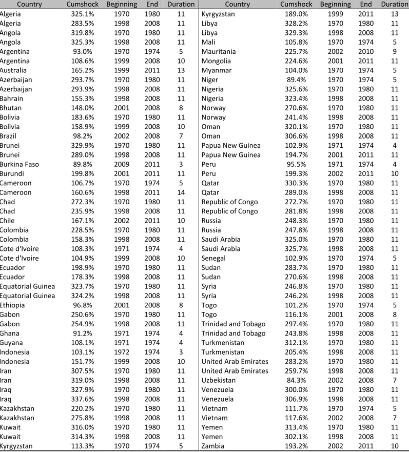
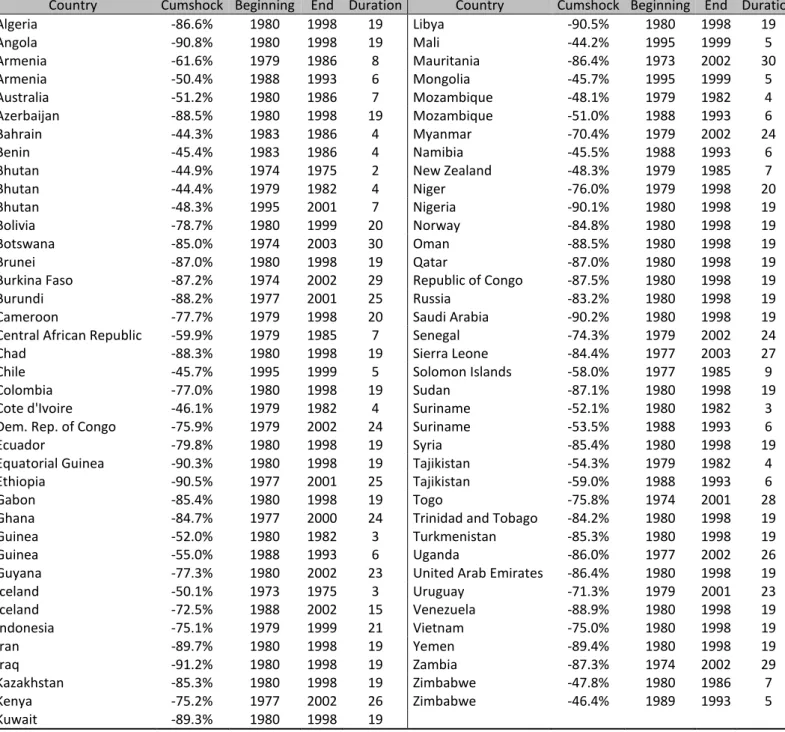
To tackle this problem, we test for each year whether our adjusted cumulative commodity price shocks between the beginning and the end of the tested period still remain above the selected threshold of cumulative commodity price shocks. We perform these tests for years earlier and beyond the first selected period until the adjusted cumulative commodity price shock fall below the threshold. While this modification catches more relevant episodes it extends our selection of episodes further than necessary so we restrict the time periods from troughs to peaks or conversely. The resulting sample presented in table 1 and 2 consists of 94 commodity price booms episodes in 56 countries and of 77 commodity price busts episodes in 68 countries.
34 While one could think this threshold would poorly select commodity price episodes, we should remind that 10% of positive
(negative) commodity price observations consists approximatively of 5% of our data sample because cumulative price shocks observation only includes positive (negative) commodity price variations. Moreover, some episodes include multiple
observations of cumulative commodity price shocks above our threshold which incited us to select a less binding threshold. The threshold values for the cumulative shock are respectively +84.3% and -44.2%.
Country Cumshock Beginning End Duration Country Cumshock Beginning End Duration Algeria 325.1% 1970 1980 11 Kyrgyzstan 189.0% 1999 2011 13 Algeria 283.5% 1998 2008 11 Libya 328.2% 1970 1980 11 Angola 319.8% 1970 1980 11 Libya 329.3% 1998 2008 11 Angola 325.3% 1998 2008 11 Mali 105.8% 1970 1974 5 Argentina 93.0% 1970 1974 5 Mauritania 225.7% 2002 2010 9 Argentina 108.6% 1999 2008 10 Mongolia 224.6% 2001 2011 11 Australia 165.2% 1999 2011 13 Myanmar 104.0% 1970 1974 5 Azerbaijan 293.7% 1970 1980 11 Niger 89.4% 1970 1974 5 Azerbaijan 293.9% 1998 2008 11 Nigeria 325.6% 1970 1980 11 Bahrain 155.3% 1998 2008 11 Nigeria 323.4% 1998 2008 11 Bhutan 148.0% 2001 2008 8 Norway 270.6% 1970 1980 11 Bolivia 183.6% 1970 1980 11 Norway 241.4% 1998 2008 11 Bolivia 158.9% 1999 2008 10 Oman 320.1% 1970 1980 11 Brazil 98.2% 2002 2008 7 Oman 306.6% 1998 2008 11
Brunei 329.9% 1970 1980 11 Papua New Guinea 102.9% 1971 1974 4
Brunei 289.0% 1998 2008 11 Papua New Guinea 194.7% 2001 2011 11
Burkina Faso 89.8% 2009 2011 3 Peru 95.5% 1971 1974 4
Burundi 199.8% 2001 2011 11 Peru 199.3% 2002 2011 10
Cameroon 106.7% 1970 1974 5 Qatar 330.3% 1970 1980 11
Cameroon 160.6% 1998 2011 14 Qatar 289.0% 1998 2008 11
Chad 272.3% 1970 1980 11 Republic of Congo 272.7% 1970 1980 11
Chad 235.9% 1998 2008 11 Republic of Congo 281.8% 1998 2008 11
Chile 167.1% 2002 2011 10 Russia 248.3% 1970 1980 11
Colombia 228.5% 1970 1980 11 Russia 247.8% 1998 2008 11
Colombia 158.3% 1998 2008 11 Saudi Arabia 325.0% 1970 1980 11
Cote d'Ivoire 108.3% 1971 1974 4 Saudi Arabia 325.7% 1998 2008 11
Cote d'Ivoire 104.9% 1999 2008 10 Senegal 102.9% 1970 1974 5
Ecuador 198.9% 1970 1980 11 Sudan 283.7% 1970 1980 11
Ecuador 178.3% 1998 2008 11 Sudan 270.6% 1998 2008 11
Equatorial Guinea 323.7% 1970 1980 11 Syria 246.8% 1970 1980 11
Equatorial Guinea 324.2% 1998 2008 11 Syria 246.2% 1998 2008 11
Ethiopia 96.8% 2001 2008 8 Togo 101.2% 1970 1974 5
Gabon 250.6% 1970 1980 11 Togo 116.1% 2001 2008 8
Gabon 254.9% 1998 2008 11 Trinidad and Tobago 297.4% 1970 1980 11
Ghana 91.2% 1971 1974 4 Trinidad and Tobago 243.8% 1998 2008 11
Guyana 108.1% 1971 1974 4 Turkmenistan 312.1% 1970 1980 11
Indonesia 103.1% 1972 1974 3 Turkmenistan 205.4% 1998 2008 11
Indonesia 151.7% 1999 2008 10 United Arab Emirates 283.2% 1970 1980 11
Iran 307.5% 1970 1980 11 United Arab Emirates 259.7% 1998 2008 11
Iran 319.0% 1998 2008 11 Uzbekistan 84.3% 2002 2008 7 Iraq 327.9% 1970 1980 11 Venezuela 300.0% 1970 1980 11 Iraq 337.6% 1998 2008 11 Venezuela 306.9% 1998 2008 11 Kazakhstan 220.2% 1970 1980 11 Vietnam 111.7% 1970 1974 5 Kazakhstan 275.8% 1998 2008 11 Vietnam 117.6% 2002 2008 7 Kuwait 316.0% 1970 1980 11 Yemen 313.4% 1970 1980 11 Kuwait 314.3% 1998 2008 11 Yemen 302.1% 1998 2008 11 Kyrgyzstan 113.3% 1970 1974 5 Zambia 193.2% 2002 2011 10
Table 1: Commodity price boom episodes
Cumshock: Refers to the cumulative price growth from the beginning to the end of each episode
Country Cumshock Beginning End Duration Country Cumshock Beginning End Duration Algeria -86.6% 1980 1998 19 Libya -90.5% 1980 1998 19 Angola -90.8% 1980 1998 19 Mali -44.2% 1995 1999 5 Armenia -61.6% 1979 1986 8 Mauritania -86.4% 1973 2002 30 Armenia -50.4% 1988 1993 6 Mongolia -45.7% 1995 1999 5 Australia -51.2% 1980 1986 7 Mozambique -48.1% 1979 1982 4 Azerbaijan -88.5% 1980 1998 19 Mozambique -51.0% 1988 1993 6 Bahrain -44.3% 1983 1986 4 Myanmar -70.4% 1979 2002 24 Benin -45.4% 1983 1986 4 Namibia -45.5% 1988 1993 6
Bhutan -44.9% 1974 1975 2 New Zealand -48.3% 1979 1985 7
Bhutan -44.4% 1979 1982 4 Niger -76.0% 1979 1998 20
Bhutan -48.3% 1995 2001 7 Nigeria -90.1% 1980 1998 19
Bolivia -78.7% 1980 1999 20 Norway -84.8% 1980 1998 19
Botswana -85.0% 1974 2003 30 Oman -88.5% 1980 1998 19
Brunei -87.0% 1980 1998 19 Qatar -87.0% 1980 1998 19
Burkina Faso -87.2% 1974 2002 29 Republic of Congo -87.5% 1980 1998 19
Burundi -88.2% 1977 2001 25 Russia -83.2% 1980 1998 19
Cameroon -77.7% 1979 1998 20 Saudi Arabia -90.2% 1980 1998 19
Central African Republic -59.9% 1979 1985 7 Senegal -74.3% 1979 2002 24
Chad -88.3% 1980 1998 19 Sierra Leone -84.4% 1977 2003 27
Chile -45.7% 1995 1999 5 Solomon Islands -58.0% 1977 1985 9
Colombia -77.0% 1980 1998 19 Sudan -87.1% 1980 1998 19
Cote d'Ivoire -46.1% 1979 1982 4 Suriname -52.1% 1980 1982 3
Dem. Rep. of Congo -75.9% 1979 2002 24 Suriname -53.5% 1988 1993 6
Ecuador -79.8% 1980 1998 19 Syria -85.4% 1980 1998 19
Equatorial Guinea -90.3% 1980 1998 19 Tajikistan -54.3% 1979 1982 4
Ethiopia -90.5% 1977 2001 25 Tajikistan -59.0% 1988 1993 6
Gabon -85.4% 1980 1998 19 Togo -75.8% 1974 2001 28
Ghana -84.7% 1977 2000 24 Trinidad and Tobago -84.2% 1980 1998 19
Guinea -52.0% 1980 1982 3 Turkmenistan -85.3% 1980 1998 19
Guinea -55.0% 1988 1993 6 Uganda -86.0% 1977 2002 26
Guyana -77.3% 1980 2002 23 United Arab Emirates -86.4% 1980 1998 19
Iceland -50.1% 1973 1975 3 Uruguay -71.3% 1979 2001 23 Iceland -72.5% 1988 2002 15 Venezuela -88.9% 1980 1998 19 Indonesia -75.1% 1979 1999 21 Vietnam -75.0% 1980 1998 19 Iran -89.7% 1980 1998 19 Yemen -89.4% 1980 1998 19 Iraq -91.2% 1980 1998 19 Zambia -87.3% 1974 2002 29 Kazakhstan -85.3% 1980 1998 19 Zimbabwe -47.8% 1980 1986 7 Kenya -75.2% 1977 2002 26 Zimbabwe -46.4% 1989 1993 5 Kuwait -89.3% 1980 1998 19
Table 2: Commodity price bust episodes
Cumshock: Refers to the cumulative price growth from the beginning to the end of each episode
4. Empirical results
4.1. Cointegration analysis
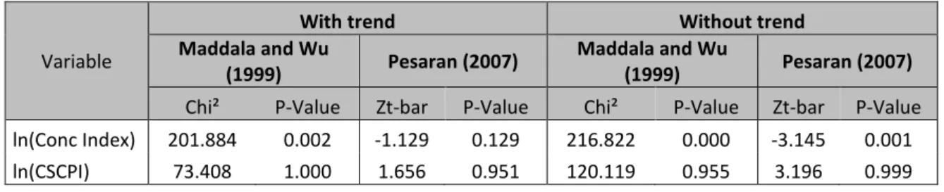
To begin with, table 3 provides some estimates of panel unit root tests on our interest variables using the Maddala and Wu (1999) test and the cross-section dependence robust Pesaran (2007) test. Thanks to dynamic unreported results we have set the number of lags to 2 without a trend for CSCPI and to 1 for our concentration index with a trend.
While the results unanimously fail to reject the unit root hypothesis for ln(CSCPI), the results are mixed for our concentration index. In fact, the Maddala and Wu test (1999) rejects the presence of a unit root test, while the Pesaran test fails to reject the unit root hypothesis on the specification with trend but reject it on the specification without trend. Due to the significance of a trend in the concentration index data process and to the importance of cross-section dependence35 in our sample we rely on the estimates that fails to reject the hypothesis of a unit root even though it is the only reported result which do so.
Variable
With trend Without trend
Maddala and Wu
(1999) Pesaran (2007)
Maddala and Wu
(1999) Pesaran (2007)
Chi² P-Value Zt-bar P-Value Chi² P-Value Zt-bar P-Value
ln(Conc Index) 201.884 0.002 -1.129 0.129 216.822 0.000 -3.145 0.001
ln(CSCPI) 73.408 1.000 1.656 0.951 120.119 0.955 3.196 0.999
We now turn our attention to the estimation of the potential cointegration relationship on different country
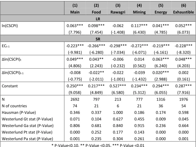
grouping in table 4. For every specification we fail to reject the difference between the coefficients estimated thanks to the MG model and those estimated with the PMG which seems to validate the hypothesis of long-run coefficients homogeneity. Regarding the Westerlund cointegration tests, it is striking to realize that we reject the hypothesis of no cointegration for the whole panel for our main regression as well as with our energy and exhaustible equations. However, we fail to reject the no cointegration hypothesis for the 4 test statistics with the food, raw agricultural materials and mining groupings.
When looking at the PMG estimates, we remark that the speed of adjustment is significantly negative which is the sign of a strong reversion towards the long-run relationship36. Moreover, the long run coefficient for the CSCPI variations is always significantly positive apart from the raw agricultural materials estimation. Regarding the short-run impact of CSCPI variations we find a significant positive impact aside from raw agricultural materials and mining regressions, while the lagged variations are only significant twice and have an impact from two to three times weaker on the concentration index. As a result, we won’t introduce lagged variations of CSCPI in the analysis and will keep on with the contemporaneous variation. We could also note that only for the energy category the short run coefficient exceeds the long run coefficient but this point necessitates further analysis in order to deduce something consistent about it.
To sum up, commodity dependent countries have experienced both a short-run and a long-run relationship which leads to a concentration of exports following a commodity price increase or a diversification of exports following a
35 We have performed some unreported Pesaran (2004) tests which strongly reject the hypothesis of cross-section
independence in our panel.
36 The speed of adjustment -0.223 in the main specification corresponds to a duration of 2.75 years in order to eliminate 50% of
an exogenous shock (often referred as the half-life) and 5.49 years in order to eliminate 75%.
Table 3: Panel unit root tests
commodity price drop. However, as evidenced by our results this effect may be triggered by producers of exhaustible resources, especially hydrocarbon producers.
(1) (2) (3) (4) (5) (6)
Main Food Rawagri Mining Energy Exhaustible LR ln(CSCPI) 0.063*** 0.098*** -0.062 0.117*** 0.041*** 0.052*** (7.796) (7.454) (-1.408) (6.430) (4.785) (6.073) SR ECt-1 -0.223*** -0.266*** -0.298*** -0.272*** -0.219*** -0.228*** (-9.981) (-6.280) (-7.034) (-6.071) (-6.161) (-8.320) ∆ln(CSCPI)t 0.049*** 0.043** -0.006 0.014 0.063*** 0.048*** (4.806) (2.243) (-0.232) (0.562) (6.240) (4.203) ∆ln(CSCPI)t-1 -0.008 -0.022** -0.022 -0.039 0.020*** 0.002 (-0.775) (-2.011) (-1.001) (-1.432) (2.988) (0.161) Constant 0.250*** 0.217*** 0.527*** 0.234*** 0.294*** 0.287*** (9.058) (4.849) (6.580) (5.312) (6.055) (7.916) N 2692 797 213 777 1316 1976 N of countries 74 21 6 21 36 54 Hausman (P-Value) 0.346 0.337 1.000 0.186 0.174 0.598
Westerlund Gt stat (P-Value) 0.071 0.104 0.627 0.455 0.009 0.045
Westerlund Ga stat (P-Value) 0.806 0.681 0.840 0.915 0.236 0.664
Westerlund Pt stat (P-Value) 0.000 0.252 0.177 0.143 0.000 0.000
Westerlund Pa stat (P-Value) 0.001 0.235 0.304 0.261 0.000 0.001
* P-Value<0.10, ** P-Value <0.05, *** P-Value <0.01
4.2. Common correlated effects estimators
4.2.1. Main estimations
While the previous section has evidenced a positive relationship between commodity price variations and export concentration both in the short run and in the long run, this model fails to take into account the global common factors impacting differently every country through both dependent and independent variables of our model, which motivates the analysis of our CCEMG results.
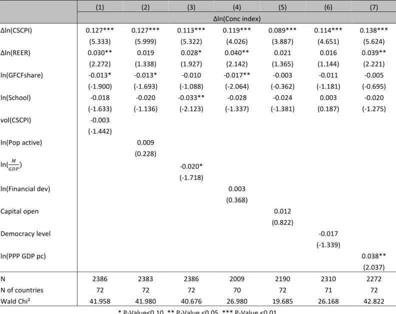
In table 5.1, we find a strongly significant positive and stable impact of CSCPI variations on the evolution of our export concentration index across every specification. The average coefficient of 0.118 across our 7 columns show that a 10% increase in commodity prices is associated to a slightly more than 1% increase in export concentration37. Even though this quantitative impact may seem low, we should remind that it corresponds only to the
contemporaneous response to commodity price variations. The analysis of commodity price booms and busts episodes in next section will take into account longer-run effects on diversification. We should also note that REER appreciation and a decrease in the GFCF share are also slightly linked with export concentration.
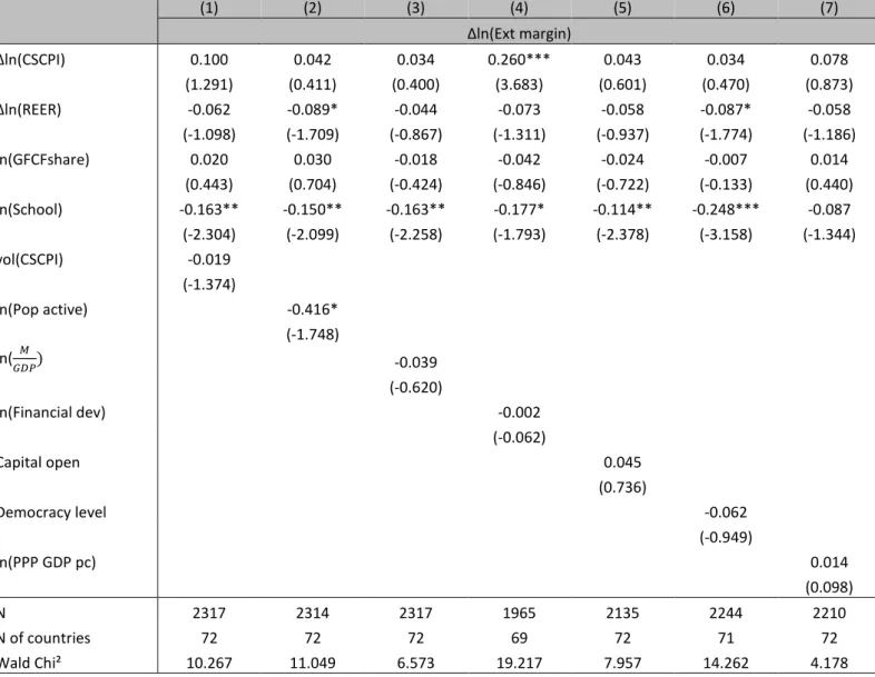
The pattern is quite identical regarding estimates based on the intensive margin index in table 5.2 but with a more salient impact of REER appreciations. However, in table 5.3 CSCPI variations only impact the extensive margin index
37 The interpretation could also be reversed with a 10% decrease in commodity prices being associated with a slightly more than
1% decrease in export concentration (or increase in export diversification).
Table 4: Pool Mean Group (PMG) estimations 𝐸𝐶𝑡−1: Error correction term
Hausman (P-Value): P-Value for the Hausman test of the non-systematic difference between the coefficients for the MG and PMG estimates. The upper part of the table refers to the long-run relationship (LR) while the bottom part refers to the short run coefficients (SR).
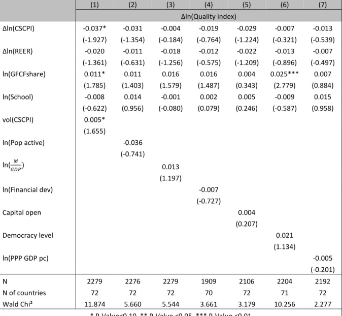
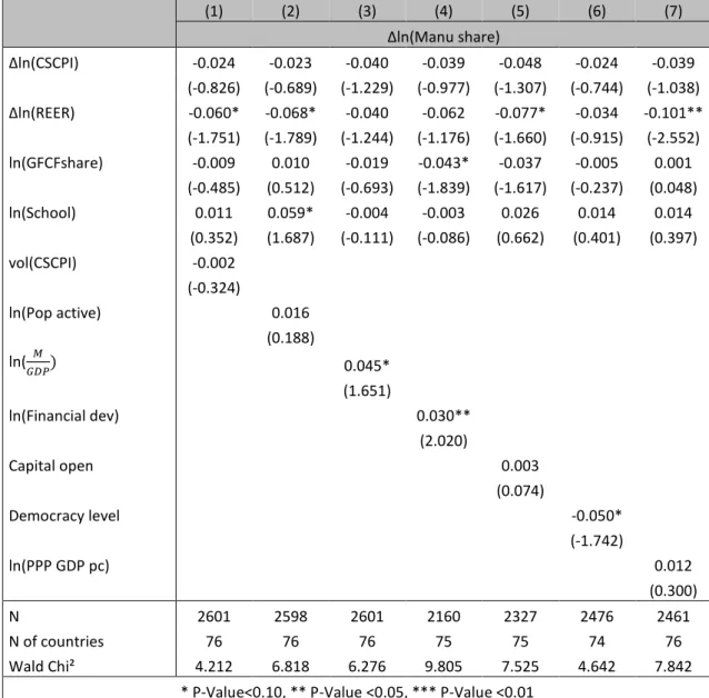
when the financial development is included in the regression, while improvements in the stock of human capital seem to be the main determinants of extensive diversification, that is to say the creation of new exports lines. Finally, our model fails to explain correctly the variations of the relative quality of exported goods in table 5.4 as well as the evolution of the manufacturing value-added share in table 5.5, even though we find some consistent impact of REER depreciation on manufacturing value-added share growth.
(1) (2) (3) (4) (5) (6) (7) ∆ln(Conc index) ∆ln(CSCPI) 0.127*** 0.127*** 0.113*** 0.119*** 0.089*** 0.114*** 0.138*** (5.333) (5.999) (5.322) (4.026) (3.887) (4.651) (5.624) ∆ln(REER) 0.030** 0.019 0.028* 0.040** 0.021 0.016 0.039** (2.272) (1.338) (1.927) (2.142) (1.365) (1.144) (2.221) ln(GFCFshare) -0.013* -0.013* -0.010 -0.017** -0.003 -0.011 -0.005 (-1.900) (-1.693) (-1.088) (-2.064) (-0.362) (-1.181) (-0.695) ln(School) -0.018 -0.020 -0.033** -0.028 -0.024 0.003 -0.020 (-1.633) (-1.136) (-2.123) (-1.337) (-1.381) (0.187) (-1.275) vol(CSCPI) -0.003 (-1.442) ln(Pop active) 0.009 (0.228) ln( 𝑀 𝐺𝐷𝑃) -0.020* (-1.718) ln(Financial dev) 0.003 (0.368) Capital open 0.012 (0.822) Democracy level -0.017 (-1.339) ln(PPP GDP pc) 0.038** (2.037) N 2386 2383 2386 2009 2190 2310 2272 N of countries 72 72 72 70 72 71 72 Wald Chi² 41.958 41.980 40.676 26.980 19.685 26.168 42.822
* P-Value<0.10, ** P-Value <0.05, *** P-Value <0.01
Table 5.a: Mean-Group Common-correlated effects (CCEMG) estimates for the concentration index
The constant is not reported in the table above
(1) (2) (3) (4) (5) (6) (7) ∆ln(Int margin) ∆ln(CSCPI) 0.089*** 0.116*** 0.102*** 0.122*** 0.098*** 0.114*** 0.117*** (3.553) (4.706) (4.530) (4.300) (4.391) (4.549) (4.250) ∆ln(REER) 0.053*** 0.031* 0.047** 0.054*** 0.017 0.023 0.035** (3.309) (1.798) (2.510) (2.960) (0.979) (1.329) (2.114) ln(GFCFshare) -0.014* -0.012 -0.018 -0.016 -0.006 -0.011 -0.011 (-1.950) (-1.515) (-1.442) (-1.638) (-0.676) (-1.042) (-1.382) ln(School) 0.019 0.031 0.040* -0.028 -0.002 0.033* 0.012 (1.178) (1.229) (1.932) (-1.088) (-0.092) (1.813) (0.639) vol(CSCPI) -0.005* (-1.733) ln(Pop active) 0.122** (2.365) ln( 𝑀 𝐺𝐷𝑃) -0.013 (-0.771) ln(Financial dev) 0.001 (0.149) Capital open 0.029 (1.092) Democracy level -0.017 (-1.166) ln(PPP GDP pc) 0.023 (0.980) N 2386 2383 2386 2009 2190 2310 2272 N of countries 72 72 72 70 72 71 72 Wald Chi² 31.766 34.782 33.229 31.141 21.892 28.189 25.812
* P-Value<0.10, ** P-Value <0.05, *** P-Value <0.01
Table 5.b: Mean-Group Common-correlated effects (CCEMG) estimates for the intensive margin index
The constant is not reported in the table above
(1) (2) (3) (4) (5) (6) (7) ∆ln(Ext margin) ∆ln(CSCPI) 0.100 0.042 0.034 0.260*** 0.043 0.034 0.078 (1.291) (0.411) (0.400) (3.683) (0.601) (0.470) (0.873) ∆ln(REER) -0.062 -0.089* -0.044 -0.073 -0.058 -0.087* -0.058 (-1.098) (-1.709) (-0.867) (-1.311) (-0.937) (-1.774) (-1.186) ln(GFCFshare) 0.020 0.030 -0.018 -0.042 -0.024 -0.007 0.014 (0.443) (0.704) (-0.424) (-0.846) (-0.722) (-0.133) (0.440) ln(School) -0.163** -0.150** -0.163** -0.177* -0.114** -0.248*** -0.087 (-2.304) (-2.099) (-2.258) (-1.793) (-2.378) (-3.158) (-1.344) vol(CSCPI) -0.019 (-1.374) ln(Pop active) -0.416* (-1.748) ln( 𝑀 𝐺𝐷𝑃) -0.039 (-0.620) ln(Financial dev) -0.002 (-0.062) Capital open 0.045 (0.736) Democracy level -0.062 (-0.949) ln(PPP GDP pc) 0.014 (0.098) N 2317 2314 2317 1965 2135 2244 2210 N of countries 72 72 72 69 72 71 72 Wald Chi² 10.267 11.049 6.573 19.217 7.957 14.262 4.178
* P-Value<0.10, ** P-Value <0.05, *** P-Value <0.01
Table 5.c: Mean-Group Common-correlated effects (CCEMG) estimates for the extensive margin index
The constant is not reported in the table above
(1) (2) (3) (4) (5) (6) (7) ∆ln(Quality index) ∆ln(CSCPI) -0.037* -0.031 -0.004 -0.019 -0.029 -0.007 -0.013 (-1.927) (-1.354) (-0.184) (-0.764) (-1.224) (-0.321) (-0.539) ∆ln(REER) -0.020 -0.011 -0.018 -0.012 -0.022 -0.013 -0.007 (-1.361) (-0.631) (-1.256) (-0.575) (-1.209) (-0.896) (-0.497) ln(GFCFshare) 0.011* 0.011 0.016 0.016 0.004 0.025*** 0.007 (1.785) (1.403) (1.579) (1.487) (0.343) (2.779) (0.884) ln(School) -0.008 0.014 -0.001 0.002 0.005 -0.009 0.015 (-0.622) (0.956) (-0.080) (0.079) (0.246) (-0.587) (0.958) vol(CSCPI) 0.005* (1.655) ln(Pop active) -0.036 (-0.741) ln( 𝑀 𝐺𝐷𝑃) 0.013 (1.197) ln(Financial dev) -0.007 (-0.727) Capital open 0.004 (0.207) Democracy level 0.021 (1.134) ln(PPP GDP pc) -0.005 (-0.201) N 2279 2276 2279 1909 2106 2204 2192 N of countries 72 72 72 70 72 71 72 Wald Chi² 11.874 5.660 5.544 3.661 3.179 10.256 2.277
* P-Value<0.10, ** P-Value <0.05, *** P-Value <0.01
Table 5.d: Mean-Group Common-correlated effects (CCEMG) estimates for the relative quality index
The constant is not reported in the table above
(1) (2) (3) (4) (5) (6) (7) ∆ln(Manu share) ∆ln(CSCPI) -0.024 -0.023 -0.040 -0.039 -0.048 -0.024 -0.039 (-0.826) (-0.689) (-1.229) (-0.977) (-1.307) (-0.744) (-1.038) ∆ln(REER) -0.060* -0.068* -0.040 -0.062 -0.077* -0.034 -0.101** (-1.751) (-1.789) (-1.244) (-1.176) (-1.660) (-0.915) (-2.552) ln(GFCFshare) -0.009 0.010 -0.019 -0.043* -0.037 -0.005 0.001 (-0.485) (0.512) (-0.693) (-1.839) (-1.617) (-0.237) (0.048) ln(School) 0.011 0.059* -0.004 -0.003 0.026 0.014 0.014 (0.352) (1.687) (-0.111) (-0.086) (0.662) (0.401) (0.397) vol(CSCPI) -0.002 (-0.324) ln(Pop active) 0.016 (0.188) ln( 𝑀 𝐺𝐷𝑃) 0.045* (1.651) ln(Financial dev) 0.030** (2.020) Capital open 0.003 (0.074) Democracy level -0.050* (-1.742) ln(PPP GDP pc) 0.012 (0.300) N 2601 2598 2601 2160 2327 2476 2461 N of countries 76 76 76 75 75 74 76 Wald Chi² 4.212 6.818 6.276 9.805 7.525 4.642 7.842
* P-Value<0.10, ** P-Value <0.05, *** P-Value <0.01
Table 5.e: Mean-Group Common-correlated effects (CCEMG) estimates for the manufacturing VA share
The constant is not reported in the table above