ASYNCHRONOUS PROGRAMMABLE CONTROL STRUCTURE
by
Donald N. North and
James M. Guyer
Submitted in Partial Fulfillment of the Requirements for the Degrees of Bachelor of Science
at the
MASSACHUSETTS INSTITUTE OF TECHNOLOGY
May, 1975
Sf
Signatures of the Authors .... a...a.a. a 4...
Department of Electdical Engineering and Computer Science
Submitted May 14, 1975 Certified by ...
Thesis Supervisor Accepted by ...
Chairmn, Departmental Committee on Theses
Archives
*bSS. INST.(MAY 23 1975
THE DESIGN AND CONSTRUCTION OF AN ASYNCHRONOUS PROGRAMMABLE CONTROL STRUCTURE
by Donald North
and James Guyer
Submitted to the Department of Electrical Engineering and Computer Science on May 9, 1975 in partial fulfillment of the
requirements for the degree of Bachelor of Science ABSTRACT
This paper is concerned with the design and implementation of a practical asynchronous control structure capable of being easily programmed. Based upon an idea originally conceived by Professor Suhas S. Patil, the structure is a hardware system designed to
simulate the concept of a Petri Net and its internal flow of control. Such nets have found useful applications in the analysis of control flow in asynchronous systems; our net simulator, with its integrated interface circuitry to external functional subsystem building blocks, can provide the control structure for an arbitrary asynchronous system.
Two versions are described in this paper. The first system, currently under construction, is a prototype medium scale programmable matrix, designed to be directly compatible with the other asynchronous modules in use at the Computation Structures Group Lab, and thus easily
interface to the outside world. Note that this entire functional system contains no clocks at all; its inherent speed is solely a function of the logic family used in its construction. Specific details are presented on the complete design , implementation and use of the control structure. The second version is a paper study
only of the feasibility of using a smaller programmable matrix ( such as above ) plus some additional control circuitry to simulate a much
larger matrix through time multiplexing. The advantages and dis-advantages of this approach are explored.
THESIS SUPERVISOR: Professor Suhas S. Patil
ACKNOWLEDGEMENTS
We would like to thank Professor Patil for his ideas about a programmable logic array, which formed the basis for our project, and for his further help as work progressed, especially concerning
TABLE OF CONTENTS Title
Page...
Abstract... Acknowledgements... Table of Contents... List of Illustrations... Introduction... ... e... ... e.... ... ... g... .. e...I. The Petri Net.... *. ... . .9
A. The Petri NetMode... B. Our Control Structure Model... C. Typical Net Constructions... D. Matrix Notation for Petri Nets. II. The Programmable Array... A. The Switching Matrix... B. The Implementation... C. The Register Matrix... III. The Multiplexed Array...e A. The Multiplexing Technique... B. Implementing the Array... C. The Memory Controller... Conclusion....*...ee..e.. ... ... ... ... ... ... .g... .... .... .... ... .23 .. e...g....g...35 .e... ... ...38 .. g...g...47 ... 69 ... 77 e... ee ... ee...78 .... e .. ... ee...94 References. .g..e.. . . . .. . ... g gg . .... ... ... ... 104 e.. ... ... ... ... ... .... ... ... ... ... ge .. .. .e. .. .... .. .g. .e. e.. ... Page ... 1 ... 2 . ...4 e...7.. . . .. ....
LIST OF ILLUSTRATIONS
Number Title Page
I-1 Representation of places and transitions 11
1-2 A sample Petri net 12
1-3 Places and tokens in a safe net 14
1-4 The steps in the firing of a transition 15 I-5 Representation for the input-output place 18 1-6 Filling/emptying of an input-output place 20
1-7 The decision places 21
1-8 Filling/emptying of a decision place 22 1-9 Creating tokens with a multiple output transition 23 I-10 Merging tokens with a multiple input transition 24 I-11 Selecting paths through a multiple output place 25
1-12 An arbiter 26
1-13 Merging structure corresponding to "if then else" 27
1-14 The general path merging function 28
1-15 The lockout switch 29
1-16 Synchronizing m input to n output paths 29
1-17 Start and stop places 29
1-18 An asynchronous multiplier example 32
II-1 Overall system organization 37
11-2 Diode switching matrix 40
11-3 Substitution of transistors for diodes 42 11-4 Interfacing to and from the switching matrix 44
11-5 A simple transition 49
11-6 Example showing inadequacy of simple transition 49
Number Title Page 11-8 Situation showing necessity of arbitration 52
11-9 Final implementation of the transition 54
II-10 Emptying a transition's input places 56
II-11 The output place 58
11-12 The input place 60
11-13 Connections for transition to output place 61 11-14 Connections for input place to transition 61
11-15 The internal place 62
11-16 Connections for the internal place 64
11-17 The decision line 65
11-18 Operation of the decision line 66
11-19 The start place 68
11-20 Row-column intersection in register array 71
11-21 Register array address decoding 72
11-22 Register array address circuitry truth table 72
11-23 Generating an array program 75-76
III-1 Dividing up an array 79
111-2 Division of representative array pattern 81-82
111-3 Multiplexed array control circuitry 86
111-4 The place for the multiplexed array 90
III-5 Timing for a typical place 91
111-6 Simple transition for the multiplexed array 93 111-7 Block diagram of the memory controller 98
111-8 Memory controller circuitry 99
111-9 Timing diagram for memory controller 100
Introduction
All modern commercial computer Central Processing Unit design is based on synchronous logical realization. Not all of this is totally hardwired logic. Indeed, most CPU's use the technique of
microprogram-6
ming . In this technique a machine language instruction is not direct-ly executed-- each machine instruction causes the execution of a set of microinstructions that each perform a small part of the machine instruc-tion. These microinstructions are stored in a control memory, usually read-only, and must be fetched sequentially to complete each machine instruction. This type of realization is slower than an equivalent
com-pletely hardwired implementation of each machine instruction because of the multiplicity of microinstruction fetches that may be required to execute only one machine instruction, but it is much cheaper in two
sen-ses. First, it is very flexible, because to change the machine instruc-tion set one need only change the microprogram for each instrucinstruc-tion, which can be easily done by changing the contents of the control store.
Second, less logic is required as the microinstructions need not be very complex.
Asynchronous computation techniques, such as those pioneered by the Computation Structures Group at project MAC 2, are inherently much faster than hardwired synchronous techniques, and are particularly suited to parallel processing situations. Asynchronous techniques allow a pro-cess to proceed as fast as data can flow through the system, with no need for slack time to await clock generated timing signals. They are more expensive to implement as more hardware is generally required for an
asynchronous as opposed to an equivalent synchronous system. Theae sys-tems, however, have been attractive research subjects because of the sim-ple solutions they offer to many problems that plague synchronous systems, such as processor coordination without faults, parallel computationand others related to communication. Thus problems of synchronizing and coordinating subsystems are also solved.
While they are fast, hardwired asynchronous systems are just as inflexible as hardwired synchronous systems, thus speed increases in syn-chronous systems are much more easily implemented by upgrading logic component speed, rather then developing a new asynchronous system from
the ground up. An ideal and more attractive method would be the combin-ing in some form of asynchronous computation and microprogrammcombin-ing. This should retain the speed of asynchronous circuitry as well as its ease in handling coordination problems, plus would incorporate the flexibility of a microprogrammed system. A system such as this would be a much more practical alternative for a fast system than a hardwired asynchronous design.
I* The Petri Net
As presented in the intreduction, the use of asynchronous tech-niques in a microprogrammed cpu could lend itself to a new flexibility in design, from both the standpoints of ultimate attainable speed, and ease in the original design or subsequent modifications of the system. However, before one jumps directly into the specification and ultimate design of a system, it would be wise to have available an adequate tool
to model ( describe, specify ) the elements, and the desired function of these elements, in a completely unambiguous manner. Such tools, most likely of a mathematical nature,( i.e., as an extension of some
graph theory or formal programming language ) could then be useful, not only in the system design phase, but in further applications concerning the general theory of asynchronous systems. Hardware description lang-uages for synchronous cpus ( e.g., CDL, AHDL, LOTIS ), both hardwired and microprogrammed, currently exist and have found wide applicability in the design and implementation phases for cpus. 9
These tools are programs, generally written in some high level computer language, that simulate the operation of the desired system based upon statements describing (1) the structure ( e.g., physical char-acteristics such as register layout definitions and interconnections ) and (2) the control flow ( statements relating to the order of performing operations ) of elements in the system. If written correctly, these
simulators are applicable to both synchronous and asynchronous systems design ( LOTIS, for example ), but they generally confine the user to the
design/simulation of a specifici special purpose system, and have no extensive merit regarding general design theory. Some systems even
possess the ability to generate the requisite logic diagrams and wiring lists needed to construct the system ( the CASD hardware description language has such an ability ), but these are for hardwired, synchronous systems, and their efficiency is rather low. Such ability does not exist in any currently well known hardware description language for developing an asynchronous microprogrammed system.
To fill this gap, we will now introduce the concept of a Petri Net as a model for the control structure of an asynchronous system, as set forth by Patil in (8). Work in areas similar to this has been conducted by Jump in (5), with his "transition nets", and Holt in (4) with "occur-rence systems" ( both are actually forms of Petri nets ). The basic
theory present behind our use of the Petri Net model is not much different from either of these; however, when the actual physical implementation is described ( in later sections of this paper ), significant differences will be observed.
Specifically, Jump's cellular array does implement the required asynchronous control structure ( implicitly including the ability to
interface with external devices ) but lacking on two major points. His system (1) does not possess the ability to conditionally alter the flow through the system based upon decisions, restricting one to the same execution path on each cycle; this is judged to be a serious restriction on the usefulness of his system. And, (2) due to his design method of placing the control circuitry for the array within the array, and not at its boundaries, as we have done, its ability to be "programmed" is poor, requiring a major rewiring of the array to change the structures "program". Our system posseses both conditionals and is easily reprogrammable; and is
thus a very viable system to be used as a general purpose asynchronous control structure.
I-A. The Petri Net Model
1. Physical Structure of the Petri Net
The Petri net is fundamentally a means of representing a system, and its behaviour, through the use of a directed graph. Named after Carl Petri, its inventor, he first called them "transition nets", probably due to their use as modeling a system as a sequence of transitions between
states.
The structural elements of a Petri net consist of three items: the "place", the "transition", and the "arc". Each element has a specific function in the overall net structure. The places, to be represented by circles ( see figure I-I A ) act as the elements which record the state of
the system at a specific time. How the state is recorded will be explained shortly; it will suffice for now to say that the set of all places forms the state description of the system the net models at any instant in time.
2 2 2j P-f 2
inputs outputs inputs outputs
Fig. I-1 A) Representation of Fig. I-1 B) Representation of the "place". the "transition".
The transition, represented by a vertical bar,( see figure I-1 B ) is the active element in the net, as they direct the control flow through the net, altering the state of the places as the "computation" the net is performing proceeds in time. The physical structure of the net ( i.e. its morphology
)
is determined by the directed arcs ( arrows ) in the net's construction. These arcs are used to specify the inputs and outputs of each place and transition in the net. By design, arcs connect places to transitions ( and likewise transitions to places ). Logical sense precludes the possibility of connecting like elements ( e.g., place to place ).
As a syntactic convention, places whose arcs connect from the
place to a transition are referred to as "input places to the transition". Corresponding arcs originating at a transition and terminating at a place specify the "output places of the transition". Similar definitions exist for the input transitions to a place, and the output transitions of a place. In general it may be inferred from figure I-1 that both transitions and places may have an arbitrary number of input and output places and tran-sitions, respectively. Note that each transition and place must have at least one of each, however. Based upon these construction rules, figure 1-2 displays a sample Petri net.
2. The Flow of Control through the Petri Net
Representing the flow of control through a net consists of
(1) specification of the structure of the net ( by places, transitions, and arcs, as above ), and (2) the use of "tokens" to model the actual asynchronous control signals proceeding through the system. The token will represent the presence of a signal at that point in the net where it is held by a place. ( Thus the appropriate name for the places - as "places where tokens may be held"
)
In the most general type of Petri net, a given place may possess any integer number of tokens ( assumed positive, i.e., 0, 1, 2, ... ) We will restrict ourselves, however, to a system in which each place can contain either zero ( "empty" ) or one ( "full" ) token. This restriction simplifies both the implemen-tation of places and transitions; and as will be shown shortly, causes little loss in generality ( at the expense of some complexity ) of the classes of systems which can be represented by our schema. Such nets will be termed "safe" nets. Figure 1-3 details the schematic repre-sentation of places as they can appear in a safe net. Note also that at initialization time of the net that places may start in either the full or empty state. Initially empty places will generally be used as normal elements to pass along the control signals; initially full places will most often be used for semaphore and resource sharing applications. Further uses in this area will be discussed later in section I-C.Control flow is directed through the net by the "firing" of tran-sitions. This action shifts tokens between places, thus altering the state of the system
,
allowing the computation specified by the net to proceed accordingly. The rule for firing a transition is extremely simple:A. A full place ( 1 token ) B. An empty place ( 0 tokens )
Figure 1-3) Places and tokens in a safe net.
if all the input places to the transition are full, then the transition is 'enabled to fire'. For any other combination of tokens in the input places of this transition, the transition is held in the wait state, disabled from firing until the above requirement is met. Firing a tran*
sition then consists of the following operations: (1) simultaneously removing the tokens from each input place of the firing transition
( going from full to empty ), and when this is done, (2) placing a token in each output place of the transition ( going from empty to full ). This algorithm implicitly assumes the safeness of the net construction: all the output places must be in the empty state when the transition is
enabled to fire; if this cannot be guaranteed, the net is unsafely constructed, allowing the possibility for two ( or more ) tokens to attempt to occupy the same place simultaneously. Figure 1-4 details the
sequence for the firing of a multiple input and output transition.
Notice that there are no time constraints imposed upon the time required to fire a given transition,,nor on the time that a token may reside in a place. These observations are fundamental to the asynchronous
modeling ability of the Petri net structure.
A. Transition Ti is held in the wait state,
as not all the input places Pi to Pn are full.
Ti
B. All the input places Pj to transition T, are now full; the transition is enabled to fire.
rl Q1
C. Transition T1 has completed firing; all the input
places PI to Pn are emptied, all the output places Qi to Qm are filled.
that this property is a fundamental requirement of the nets in our system. If an unbounded number of tokens could exist in any place, then any
practical implementation would require an infinite capacity counter at each place to record its state; this is clearly not realizable in a real system. If we assume that the number of tokens at any place is at least bounded by some number 2, then we can ( by implementing an n-stage binary counter at the unsafe place, through transitions ans safe places ) transform any n-bounded unsafe net of this type to a functionally equivalent safe net. Through this process we can then represent any finite state system ( which can be modeled by a n-bounded unsafe net ) as a safe net, and therefore able to be simulated by our system. Section I-C, "Typical Net Construc-tions", details the functions that can be represented by the possible place-transition interconnections, and which of these can lead to problems regarding the safeness of the entire net.
Technically, safeness can be defined as, given an initial place-ment of tokens throughout the net ( the "initial configuration" ), then a net is said to be "safe" if and only if any firing sequence of transi-tions yields no more than one token per place. In a large system, this can be a difficult criteria to establish; verifying safeness on the "sub-system level" and proceeding upward seems much more viable ( a structured programming type approach ). Safeness is best gained by careful speci-fication and design of the system; intuition also seems to help.
I-B. Our Control Structure Model
The previous Petri net model for asynchronous systems provides a good theoretical base for system design and analysis. However, several important features are lacking which would be necessary to fully utilize the net facility to actually implement a useful asynchronous system in "hardware".
The two major functions that need to be added to our system are (1) interfacing to the outside world, and (2) a method of altering the sequence of control based upon signals obtained from outside the matrix. With these added abilities, our matrix is then able to function with the equivalent functional complexity of the control circuitry of a cpu.
1. Communication with the Outside World
Implementation of communication links with external systems
( circuits ) is desired along the lines ( for compatibility ) as first developed by Patil and his macro-modular asynchronous building blocks
in (6) and Patil and Dennis' asynchronous modules in (2). In this manner asynchronous control signals can be passed to and from our simulator, so that it looks to the other modules as just another module in the system, freely interchangeable
Signals in this asynchronous modular system consist of transitions
(
not to be confused with the transition in the Petri net ) on the control wires from 0 ( low ) to I ( high ) or I to 0; each is a completely equiv-alent signal-:#- the change in level represents the signal. To be able totransmit and receive this signal, we have expanded the definition of a place to include a new subtype, called an "input-output place" ( or i/o-place ); the old place will henceforth be referred to as an "internal
place".
The input-output place will be represented by the square as in figure 1-5. This place actually consists of two halves: the output half, which transmits the "ready" signal ( the level change, referred to earlier )
from the matrix control structure, along a control line, to the external asynchronous module; and the input half, which receives the corresponding
"acknowledge" signal from the external module and enters it into the matrix.
( Note - we will not attempt here to enter into a full discussion concerning the ready/acknowledge signalling conventions that will be used. The reader is referred to reference (2) for Dennis' and Patil's presentation of this topic and its use with the asynchronous modular system. )
This new place can replace any previous titernal place in the Petri net structure; if it is desired to perform some external function at that time in the net's "computation". The internal place's function is now to act only as an internal status indicator within the confines of the matrix
( thus the name "internal" ). The input-output place is used to asynchro-nously activate external devices connected to the matrix; the internal place for such uses as resource sharing or lock-type semaphores.
output half input half 1N Ix 1 2 >2 inputs outputs m n
Mechanically, the filling and emptying of the input-output place is directly compatible with that of the internal place, to insure their direct substitutibility. The i-o place works as follows: Assume it is initially in the empty state ( it will be at system initialization, as all control links, and thus the i-o place, are reset to the inactive state at this time ). Now let a transition, of which this is an output place, fire; thus a token will attempt to enter into this place. As this operation begins, the token enters the 6utputa( left ) half, and immediately a ready signal ( transition, level change ) is sent along the place's control link on the ready wire. The "official" state of the place is still empty, so as not to fire any transitions attached to its input ( right ) half prematurely; but the control link is in the active state now, and presumably the device attached to the link is performing its operation. Some arbitrary time later ( after it finishes ), the corresponding acknowledge signal is returned on the acknowledge wire, indicating the external device has finished. The link now enters the itiactive state, and the i-o place then enters the full state, indicating
the presence of a token. At this point, its behavior is exactly the same as an internal place. Subsequently, its token will be removed by a transition being fed by this place, resetting it to the empty state, ready to begin another cycle. Thus communication with external devices
or systems ( possibly even another matrix such as this one ) is handled in a very clean asynchronous manner, compatible with the previously developed signaling criteria. Figure 1-6 details a typical portion of a net containing an input-output place, and the flow of control that results
r+ ia
P1 TP2 P3
A. Internal place PI contains a token; transition T1 enabled to fire.
Ready/acknowledge link on i-o place P2 is inactive. *** I
ri a
P1 Tj P2 T2 P3
B. Transition T1 has fired; token placed in output half of i-o place P2;
ready signal sent on control link; transition T2 not yet enabled.
ri a
P1
Tj IP2 T2 P3C. Acknowledge signal received on control link; token placed in input half of i-o place P2; transition T2 now enabled to fire.
t I
P1.TjP T2 P3
D. TrRnsition T2 has fired, token placed in internal place P
3.
Control link on place P2 is again in inactive state.
Figure 1-6) Logical sequence for the filling/emptying of an input-output place.
2. Decision Handling in the Net
The handling of decisions by the Petri net schema will again be implemented by a modification of the place structure. Decisions will be made on the simple true/false basis, which is easiest to implement and yet provides good flexibility for operating on digital binary data.
The modified notation is detailed in figure I-7A for the i-o decision place, and in figure I-7B for the internal decision place. Both work in exactly the same manner as previously presented, except the appearence of the token into the true or false branch is controlled by the appropriate decision line from the external environment. In effect the output of the decision place ( either internal or i-o ) is directed, in a mutually exclusive manner, to either the true or false brandh depending upon the status of the decision line. How this is
physically accomplished by the net simulator will be detailed in a later section on the actual physical design of the matrix circuitry. Figure 1-8 shows a sample Petri net execution of a conditional place where the decision line held a 'true* status.
inputs outputs inputs outputs
T. T
A. Representation of the B. Representation of the input-output decision place. internal decision place. Figure 1-7) The decision places.
El il 9P2 ----T2 P3 T P1 Tl J2 ~ F P4 T2 P3 I---P1TP)V~ P1 Tj P2 A. Place P1 contains a token; transition Tl enabled to fire.
B. Transition Ti has fired; decision line
affect-ing placement of token
C. Token placed according to decision ( true ); transition T2 enabled to fires transition T3 held in wait state
D. Transition T2 has fired
Figure I-8) Logical sequence for the filling/emptying of a decision place. ( Internal place used in example; could equally well have been an input-output place for P2. )
I-C. Typical Net Constructions
Present in the complete repetoire of possible place-transition interconnections are several constructions that deserve special mention, either due to their usefulness in illustrating a specific point, or
displaying a necessary restriction on the class of nets that can be represented by a 'safe' system.
1. Creating Tokens
Tokens can be created for use on concurrent execution paths through the use of a transition with multiple outputs, as in figure 1-9. This operation is analogous to the "fork" operation used in other asynchronous system descriptions. Note that this function illustrates that the conservation of tokens, by number, is not required on the level of a single transition ( tokens will only be conserved if the number of input places equal the number of output places for that tran-sition ). However, for the net to remain safe, these tokens must
somehow be collected at some later time and merged, so that around any loop in the net it is a necessary condition that tokens be conserved, but not in general sufficient. Sufficiency will be guaranteed by correct
( in regards to safeness ) construction of each parallil sub-branch of the loop.
SP2 P2
A. Before T1 fires B. After Ti fires
Figure 1-9) Creating tokens (concurrent paths ) with a multiple output transition.
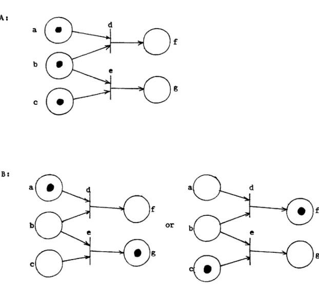
2. Merging Tokens
In a similar method to that employed above, tokens can be merged from parallel, concurrent execution paths through the use of a multiple input transition. This corresponds to the "join" or "logical and" operations employed in other systems. Note that, by definition of the transition operation, all the input places must be full before the transition is enabled to fire ( thus the logical and analogy ). Figure 1-10 illustrates concurrent path merging with a multiple input
transition.
Pi P1
0:T l
T l
P2 P2P
A. Before Ti fires B. After Ti fires
Figure I-10) Merging tokens ( concurrent paths ) with a multiple input transition.
3. Splitting Paths
The function of providing a choice of multiple execution paths in a net can be done in two manners. The first, discussed previously, provides for concurrent execution of each of a number of parallel paths through the use of a multiple output transition. This second method to be presented here enables the designer to select one of these parallel
paths to execute, either arbitrarily or by distinct choice.
Selection of a specific path from a set of choices based upon testing conditions is done using the true/false conditional places presented previously. The token will be directed to the desired branch
depending upon the status of the decision line.
An arbitrary path can be selected using the multiple output facility of a place into several different transitions. This compli-cates the firing rule for transitions, however, as there will now be
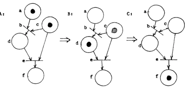
contention by the output transitions for possession of this places' token. Figure I-11 illustrates the problem. When place PO becomes full#, then by
ITj PI Tj P1 PO PO T2 P PO T2 , E T2 P2 B T P T2 P2 AT2 2
Figure I-11) Selection of mutually exclusive
paths thru a multiple output place and an arbiter.
our previous rule both transitions TI and T2 are enabled to fire. This
cannot happen, however, as we have assumed that (1) either a place is full ( one token ) or empty ( no tokens ), and (2) a transition requires a whole token for itself to fire.. We could not therefore split the token in place PO in half, and give half to each transition. To resolve this difficulty, we have created the concept of an hrbiter', which is
'attached' ( theoretically ) to all the output transitions of this place ( in theory there may be an arbitrary number, not just two as in the example ). This over-seer of the connection then arbitrarily decides which transition is able to capture the token, and subsequently fire; so that the net setup in figure I-11A can yield either the upper or lower version in I-11B after a transition fires, depending upon the 'decision'
of the arbiter. The arbiter should decide with no prejudice which transition will receive the token; all should be equally likely. How this operation is physically accomplished will be discussed in the next section on the implementation of the transition circuit.
The use of this construction is extremely important in the devel-opment of resource sharing control circuitry. For example, to lock out mutually exclusive operations,( e.g., read and write commands to a memory device ) the net structure of figure 1-12 may be used to share the resource referenced by both subnets N1 and N2. The annotation under the figure
explains its operation in detail. Note here the useful quality of being able to initially specify a place be full ( the internal place resource
sharing semaphore ).
P1 Ti T3 P3
Ni
P2< J2N T4 O P4
Figure 1-12) An arbiter. Either subnet N1 or N2 may execute based
on whether a token is present first in Pl or P2 respectively.
Presumably the operations in N1 and N2 are mutually exclusive.
If tokens arrive simultaneously, the arbiter between transitions T1 and T2 decides where the token in PO will go. The branch chosen
steals the token in Po ( a semaphore ), inhibiting execution of the other branch until it is done; when finished, it replaces the token, resetting the arbiter for the next cycle.
4. Merging Paths
At some points in the net it might be desirable to merge several paths into a common path not with an 'and# function, as previously presented for merging tokens, but rather with an 'or' function, so that a token arriving on any input branch will produce an output. This will especially be used when one of a number of concurrent paths is executed, and it is then desired to merge all these into a single main path.( i.e., rejoining mutually exclusive paths after a conditional branch; the "if cond then N, else N2 function, see figure 1-13 ). The use of a multiple input place accomplishes this function. Note however that this construction
places a constraint on the design of the net so that it remains safe. The designer must insure that control is never given to more than one of the parallel paths at any time, or indeterminacy can result, as a transition ( TI to Tn in figure 1-14 ) could then
possibly fire into a full place ( PO ). Figure 1-14 illustrates the use of the path merging function.
IN - - N PI cond P2 F N 2
Figure 1-13) Merging structure corresponding to the
P1 Tj
P2 T2
PO
Ph Tn
Figure 1-14) The general path merging function using a multiple input place. Note that only one of places PI to Pn may be full at any one time to insure safenebs of the net; i.e., that a transition will not fire into a full place ( in this case, PO ).
5. Other Useful Functions
In this section we will present some other useful constructions and functions performable by place/transition interconnections that
should be very useful in developing Petri net control systems.
Figure 1-15 details the operation of the "lockout switch". Here place P1 insures that only one token entering from P2 can get into net NI at a time. The lockout switch is reset only when the token again
leaves net N1, continuing execution with place P3* This construction is useful for applications requiring serially reusable resources, or implementing locks on control sections that must be executed in entirety without being interrupted or restarted.
Synchronization of parallel paths can be performed very cleanly with the use of a multiple input/multiple output transition. In general, with an m-input/n-output transition, one could insure that execution on each of the m input paths had been completed before starting any of the
m output paths. Figure 1-16 displays this operation.
Starting and stopping the net can be done by, respectively, a place with no inputs that is initially full ( the "start place" ), and either a place or transition with no outputs. This is a special change of the rule that each place and transition must have at least one input and one output arc$ however, these functions are convenient, and this method provides a very simple implementation. The net in figure 1-17
illustrates the use of this facility.
P2 T2 T3 P3
NI
Figure 1-15) The lockout switch. Subnet Nl is prevented from being restarted while it is executing.
P1
Ql
Tj
Figure 1-16) Synchronizing m input paths forming n output paths.
O-
~HO
I-D. Matrix Notation for Petri Nets
A very convenient matrix notation for Petri nets has been devised by Patil. Very simply, it is constructed by enumerating all the places ( including internal, input-output, and decision lines ) present in the system along the column heads of a table, and likewise all the transitions along the row heads of the table. Connections within the net are then displayed as elements in the table using the following code:
(1) an empty block, to represent no connection
(2) a dot ( ), to represent an arc from a place to a transition, (3) a cross ()), to represent an arc from a transition
to a place
Note that this code leaves out the possibility that the same place may be both an input to and an output from the same transition. However this omission causes no loss in generality ( it can easily be
simulated by using a loop of two places and two transitions ), and thus will be readily accepted, as it simplifies representation of the loop
immensely. This code and table organization easily handles all the input/output possibilities for the transition, and the internal place. each only requires only one row ( or column ) to specify its inputs and outputs. However# the table must be extended when we add the
input--output place and decision capability, as each of these requires two columns by itself to uniquely represent its function in the table using our code defined above ( and as will be seen later in the section detail-ing the actual implementation, this choice of representation simplifies the circuit requirements for the input-output place and decision lines ).
input half respectively. The first column may only contain a cross, as it may only be the output from a transition ( the output half ). The second column'( the input half ) may likewise only contain a dot, denoting its function as an input to a transition.
The decision lines similarly require two columns, one each for the true and false branches. Each column may contain only dots ( i.e., show-ing inputs to transitions ), and placed at the row intersection of the first transition(s) of each branch ( true, false ). Note that each row that contains one of these "decision dots" must also contain at least one dot under a place column, representing an arc from a place to a
transition. If there is more than one input to this transition ( a dot ) and a decision dot is also present, then this transition will fire only when all the places are full, and the decision is satisfied ( as would be expected ).
Figure 1-18 presents a complete sample system, to perform an asynchronous fixed point multiplication of two binary numbers by the "shift and add" method. Note the system operates completely asynchro-nously, as the time to perform the emputation varies with the input numbers. Figure I-18A details the data flow portion of the system. The control structure ( in Petri net form ), is presented in figure I-18B. Observe the use of several of the constructions presented previously: creating and merging parallel paths; creating and merging mutually exclusive paths; starting and stopping the net; ordering parallel and sequential operations; use of decision branches to change the flow.
The schematic representation of the control structure in figure I-18B is then easily tabulated in matrix form in figure I-18C. This matrix notation will be the basis for the "program" in the programmable version.
A. DATA FLOW
input
REG
A FAN REG + E C: reuC
CC IN A 7 dd S ift Left b input B FAN REG C. 0 ? =0 Figure -18) AShiftdasnhoosmlilefrtwbnry fift Rightf Be CONTROL FLOW ho or 13=0 T,~~T T1-+ LOAD T SRI R*A
~
Figur-0 - ) A440/8=aynh1 ouutil e f rt o i ay
Places and Decisions I
-I:
02 0 I P3o
I
I P4 C P5~I
P7 o I1 T IF D T F * X X Tj * *X
T2 * X * T3 * X *T4 *x
x
* T 5 * X X * T6 * X T7 X * * T8 Start place ( input only ) Input-output Internal place, two columns place Stop place(
output only ) Transitions Decisions,two columns each
Figure I-18C. The matrix representation of the asynchronous multiplier.
Start 0
P6 0 I1 I
Summary
This section has presented the detailed development of a tool -the Petri net, as we have modified its structure - for use as both a
theoretical and practical model for asynchronous systems. The development of its representation by the matrix form, as a type of "program" for the places ( internal, input-output, and decision attachments ) and transitions, will now be expanded, in the next section, to a hardware structure that
is capable of simulating any Petri net representable in this form. The next section is devoted to this task.
II. The Programmable Array
Design Objectives
Our goal is to design and build a practical asynchronous control structure whose program may be changed electronically. As it turns out, the array representation of Petri nets described in the previous section is an ideal basis for design. An electronic analog of this structure, with the capability of electronically altering the pattern of
intersec-tions in the array, would be able to simulate any Petri net that the array could represent. It could thus perform the actions of any control
struc-ture that the array could simulate. Thus we chose that representation as a blueprint for our design. It will have the following characteristics:
1) There will be a row of places across the top of the array,some of which will interface with the outside world via the ready-acknowledge scheme described by Dennis2 and Patil 2,6 and some of which will be
in-ternal places. To keep the structure small but still demonstrative, it was decided to design it with four
I/O places, four internal places, and two decision lines.
2) There will be a column of transitions along the right side of the array. These will be able to be input or output transitions of any place. For reasons ela-borated later, each pair of transitions will have an arbiter between them on their inputs. There will be eight transitions in the design.
3) There will be a switching matrix to route the signals (in effect, the tokens) from places through tran-sitions back to places. It will be basically ver-tical wires that are inputs and outputs from the pla-ces, and horizontal wires that are inputs and out-puts to and from the transitions. In Patil's
ori-8
ginal version, the pattern of interconnection of the vertical and horizontal wires is determined by the physical placement of diodes. The diodes are to be replaced with transistors, with the resulting ability
to make the transistors act as open circuits or as diodes by turning them off or on.
4) An array of registers will be used, the outputs of which will drive the transistors in the switching matrix. The contents of this array is alterable, and thus so is the Petri net being simulated. This
portion of the structure is expensive, and thus was a constraint on overall size.
The resulting structure (figure TI-1 shows the general layout), can simulate a wide variety of Petri nets, and thus can be used with the modules already built in the Computation Structures Laboratory to use the ready-acknowledge signalling convention to perform a number of oper-ations. The structure itself, while not being directly expandable, can be interfaced with other similar structures of any size through the I/O
control links ra ra ra ra decisions to outside
world - >
II
start place
[
I/4 lacesjjplaces
lUTUIT
T
tIU
transitions
]1
4'
Overall system organization. SWITCHING
MATRIX
REGISTER ARRAY
II-A The Switching Matrix
The specification of the Petri net to be simulated by our system lies in the interconnections enabled by the switching matrix. While the array is operating, the place and transition circuitry perform all the logical operations to simulate the desired net, with the switching matrix directing the signals. How these signals are represented and directed is the topic of this section.
Requirements
The design objectives require the switching matrix to have the ability to connect the outputs of every transition to the inputs of
every place, and the outputs of every place to the inputs of every transition. As such, the matrix is nothing more than a specialized crossbar circuit that can be individually enabled at each intersection.
Furthermore, we also desire that to easily implement the correct func-tionality of the place and transition elements: inputs to places from transitions use the 'or* function for merging signals, so that any tran-sition may fill/empty any place, without concern of what the other in-active transitions attached as inputs to the place are doing; and that
inputs to trinsitions from places use the 'and' function for ierging signals, so that all the input places of a transition must be full before it may fire, and that it fills all its output places before it finishes firing.
Implementation
At first these requirements seem prohibitive to constructing a cost effective switching matrix, but a simple method of doing so has been
developed. It works using the following signaling conventions, and the interconnection structure of figure 11-2.
For the lines to send signals from the transitions to the places, we use active high levels. Thus the level on the output line will be high ( = 1 ) only if all the connected input lines are high ( = 1 ). This implements the required 'and'ing function. Figure 11-2 can illustrate this principle. If any of input lines Ll, L2, or L3 are low ( = 0 ), output line L2 will be pulled low ( = 0 ) throvgh the forward-biased
( conducting ) diodes D2,1, D2,2, and D2,3 tespectively ( which provide isolation from one input line to another, to prevent crosstalk ). Only when all input lines are high ( = 1 ) do we get a high ( = 1 ) on the output line, as all the diodes are now in a reverse-biased,
nonconduc-ting state. Thus our active high 'and' function directs signals from places to transitions.
Similar to above, for the lines which send signals from the transitions to the places, we use active low levels. Thus the level on the output line will be low ( = 1 ) if any connected input line is low ( = 1 ). The output level will be high ( = 0 ) only if all the input lines feeding it are high ( = 0 ). This implements the required
'or'ing function. Figure 11-2 can be used again, with the same argument as above, except for now using active low levels, to direct signals from
transitions to places using the 'or' function.
Note also the other connection possibilities present. For instance, input line Ll will never affect output line L3 ( or Ll ) as there is no
diode present at the junction where they cross to pass the signal ( in figure 11-2 ). Using the technique of inserting diodes at the desired
('W
L3 +5 f 1k 4/4D 2,2 INPUT LINES (typical)Figure 11-2) A typical portion of the switching matrix. Note the orientation of the diodes to transfer zero-positive
level signals from the input to the output lines, and their ability to prevent crosstalk between input lines.
/wv r~w +5 1k D 2 L2 OUTPUT LINES (typical) +5 1k . **
IL3
7-,3 ,D 1,#2 D 3,2 r - - -Ll ,1 4A,
Lljunctions, we can thus direct the signals between the places and transitions selectively, so that any well formed Petri net structure could be represented in the switching matrix. Patil in his hardwired array discussed in (8) used just such a system ( with diodes on plugs,
that could be mechanically moved to change the net structure ).
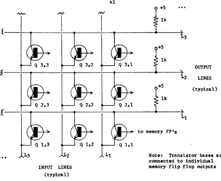
We have expanded this system in the manner illustrated in figure 11-3. At the junction of every input and output line in the matrix, we have replaced a possible hardwired diode with a transistor, oriented as in figure 11-3. The signal 'flows' through the transistor from emitter to collector, much as it 'flowed' through the diode from anode to cathode. However, the use of a transistor has an important consequence. When held in the nonconducting state ( off ), the transistor looks like an open circuit across the junction, so the input signal ( at the emitter ) has no affect on the output line ( at the collector ). Thus we have a 'no-diode' connection. Held in the conducting state ( on ), however, the
transistor now behaves like our diode placed across the junction as before, with the same influence of the input line on the output line. We now have a programmable diode at the junction.
The transistor we have used at the junction are 2N5134 type
high speed silicon NPN saturated switching transistors, which possess the desired physical characteristics, and yet are also very inexpensive.
( 9e each at this writing ). However, the use of the transistor switches
to simulate the diodes requires a memory to specify the status of each switching transistor in the array - either on, representing a diode, or off, providing an open circuit condition. TTL levels available from the memory can be used to switch these transistors very nicely. A TTL logical
AA/
Q l,2
+5
1k1
3+5
1k L2 +5S1k
OUTPUT LINES (typical)Q
2,1
xQ
1,1
Li
INPUT LINES to memory FF*sNote: Transistor bases are connected to individual memory flip flop outputs (typical)
Figure 11-3) Replacement of the hardwired diodes by transistors
results in the above structure for the switching matrix.
Q
1,3
L3 Q 22 4 I Q _3,3 J Q 3,2Q 3,1
Q 2 ,30 ( approximately +0.2 volt, and a current sink ) holds the transistor in the off, or nonconducting state, providing the open circuit, or 'no-connec-tion'. Likewise a TTL logical 1 ( approximately +3.8 volts, 1.6 mA DC current source ) provides ample base current to switch the transistor on, conducting, and establish a 'diode-connection'. The implementation of this memory circuit ( as an array of registers ) is detailed in a later section.
Interface Circuitry
We desired to finalize the design for the switching matrix as in figure 11-3, using the transistors, because this was the simplest organ-ization that provided a workable solution. However, after extensive testing to insure the correctness of our design, we found that the simple one
transistor/junction switching matrix we intended to use did not always pass TTL levels in a usable form from input to output. Thus the interface
circuitry described below is required to convert the matrix signals back to TTL compatible levels.
On an input line to the transistor matrix, we found no problems in directly interfacing our active high or low TTL levels into the switching transistors. A standard TTL gate in the low state is able to sink up to 16 mA of current, and this could easily ground the emitter connections of each transistor connected to the input line. No excessive current flow problems were found even when all the transistors on a given input line were turned on ( this amounted to about twenty transistors loading the line ). Likewise, when the TTL output was high ( +3.8 volts ), the load-ing was small enough so that no extra interface circuitry ( i.e., extra buffering ) was needed to maintain this high level, even with the maximum number of transistors ( twenty ) turned on. Figure II-4A details the
Figure 11-4 A
Input Interface: TTL logic to transistor matrix
Matrix input line TTL circuitry
F#
+3.8-+0.2_4 -L
1 2 3 A 4iLJ
L
1 2 B 3 Figure HI-4 BOutput Interface: Transistor matrix to TTL logic Matrix output I hi LM3900 line Ll 7413 +4 V + IM +3.8- +0.2-2 4 1 2 E 3 4 +3.8 -+02 4 +5 - 44-+3' TTL ircuitry
.. ... ...
2...
1
+5.0- +0.6-12 C 3 4 ~~~~~~~1 I a *A- - !3interface circuitry ( none ) and waveforms on an input line to the switching matrix. We did not investigate the problems that might be encountered with a larger number of transistors loading the input line, as would be possible in a larger switching matrix. Probably some further type of buffering of the TTL levels would be required to provide the required current sinking and open circuit high voltage capability, but
this remains to be investigated by those desiring to construct a larger array.
Problems in recovering the signal intact, as a TTL usable level, on the output lines arose, however. When only one transistor was turned on ( at the junction of the input and output lines ), the signal propo-gated intact from input to output, as was expected. However, when more than one transistor, on either the input or output lines, was turned on, a high level on input stayed at +5 volts en output, its pullup level; but a low level rose from the normal value of +0.2-0.6 volt to +3 volts. The signal was getting through, but it was level shifted upward. This effect, though we did not analyze its cause completely, seems to be due to the existence of alternate current paths through the transistors, because of their somewhat bidirectional current flow nature. The problem was not present in a system using only unidirectional flow diodes ( Patil's hardwired diode-plug array, in (8) ). The limiting value for a low was found to be +3 volts. To remedy this situation, the interface circuitry in figure II-4B was developed to convert this +5/+3 signaling system back to the standard +3.8/+0.2 TTL levels respectively. Basically just an inverting voltage comparator ( using an OP AMP ) centered at -+4 volts
reliably in breadboard versions, producing clean TTL level output ( corresponding exactly to the input ) no matter what transistors are on; at frequencies from DC to megahertz. Figure II-4B details how the waveforms pass through this interface circuitry.
Summary
We have specified here the design and practical implementation
of both a hardwired ( using diodes ) and programmable ( using transistors )
switching matrix for routing the bidirectional signals from places to transitions, that is extremely simple, yet very versatile. The next
sections will now develop the circuitry for the places and transitions, and the memory to control our transistor matrix, so that we may combine all these elements into a total Petri net simulator system.
B. The Implementation
The Switching Matrix and Signalling Constraints
The matrix consists of horizontal and vertical wires, some being inputs to the matrix, the rest being outputs. Vertical wires conduct sig-nals to and from places, and horizontal wires conduct sigsig-nals to and from transitions. As described previously, transistors are used at
intersect-ing vertical and horizontal wires to perform a logical and, function. Thus the state of each vertical output wire is the logical and of the states of each horizontal wire that is connected to it by an on transis-tor, and the state of each horizontal outnut wire is the logical and of the states of each vertical input wire that is connected to it by an on transistor. Thus the only function that the matrix can perform between its inputs and outputs is the and function. Coupled with the properties of places and transitions, this fact constrains the type of signalling that can be used between places and transitions, as explained below.
Transitions
By the definition of the transition, when it fires, it empties all of its input places, and then fills all of its output places. This would appear to require four lines from the matrix to each transition:
one to indicate when all input places are full; one to indicate when all output places are empty; one to empty all of its input places; and one to fill all of its output places. It is not too constraining on net struc-ture to require that all output places of a transition be empty when all of its input places are full. The implementation is then simplified.
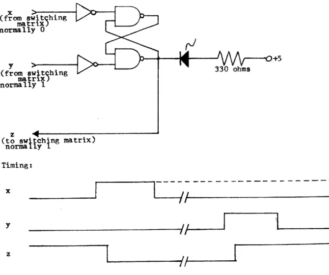
this is true and low otherwise, then one can combine the last two sig-nal wires as follows: Let there be only one input to the matrix from each transition. Since the wire indicating that all a transition's
out-put places are empty can be eliminated because of our constraint, there is only one matrix output to each transition-- the wire indicating when all its input places are full. When this wire is high (all input places are full) the input to the matrix is low. When the matrix output is low,
(some input is now empty) the matrix input from the transition is high (figure 11-5). The reasons for the inversion will be explained later. One could then design the places so that onthe high to low level change of the transition output wire that transition's input places are emptied, causing the transition input line to go low, thus causing its output line to go high, and this level change can be used to fill the transi-tion's output places.
This is not quite enough, however, Consider the situation in fig-ure 11-6. Because input places a and c are full, transition b fires, emptying places a and c. Suppose, however, that place a empties faster
than place c, so the transition input line goes low, causing transition b to place a token into place d. Place c has not yet emptied, so
transi-tion sees both its input places(d and c) full, and thus fires, putting a token into place f. The final situation should be a token in place d, however.
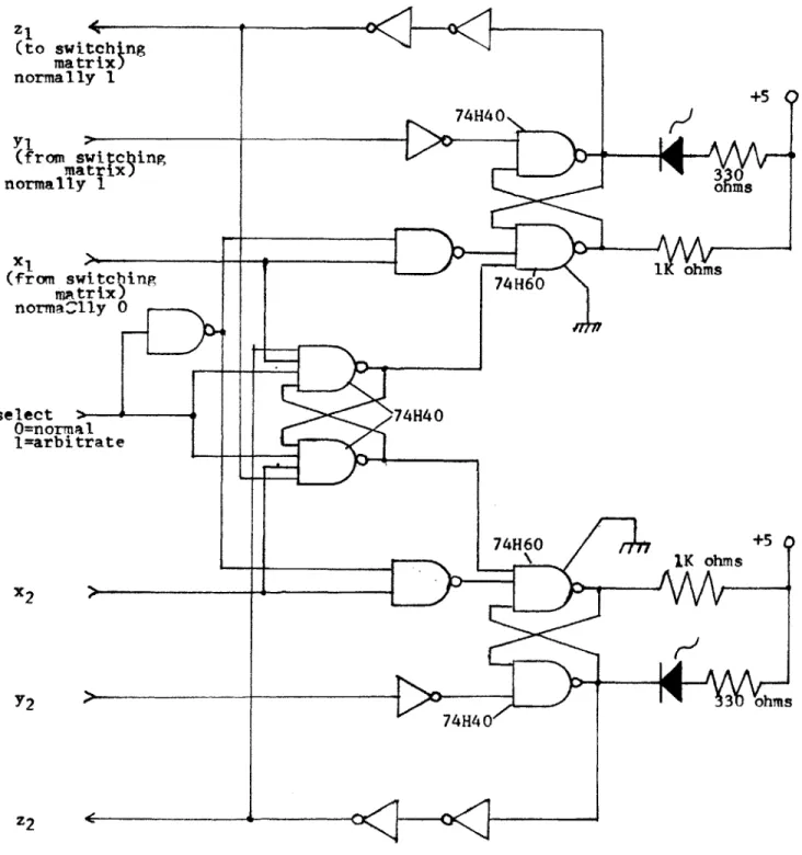
Therefore, another line is added as input to each transition. This line is high if all the input places to a transition are empty, and low otherwise. The line indicating that all input places are full is the x line. The line indicating that they are all empty is the y line, and
full indicator from > transition's input places. signal causing removal or -insertion of tokens.
Figure 1I-5. Simple transition.
A: a b c d e f B: a b c d 0f
f
C: a b c d dthe transition output line is the z line. The transition is now charac-terized by the following behavior: When line x goes high (all input pla-ces full) line y must be low (since no input plapla-ces are empty), and output line z goes from high (quiescent) to low (firing). This level change empties the input places, and as soon as one of them is empty, line x goes low. Line y goes high as soon as the last input place is emptied, then output line z goes high again, causing tokens to be placed in each output place. A complete circuit that illustrates this behavior, with its input and output lines labelled as mentioned, is shown in figure 11-7, along with a timing diagram. It includes an LED indicator to show visual-ly when the transition is firing.
This is still not quite complete, however. Consider the situation shown in figure II-8A. The tokens ina\nd c have arrived simultaneously. According to standard Petri net theory, after any action the situation should be one of the two cases shown in figure II-8B, with only one of the transitions having fired. At present, however, both transitions would be enabled as their conditions for firing would be met, and so both would fire simultaneously. It is not at all clear what the final state would be.
The situation pictured, then, calls for some sort of arbitration on the firing of transitions so situated. Inputs to the arbiter must be both the x line from each transition involved and the z line, since the x
line may go low before all the input places are empty, and one would like to keep the other transition(s) blocked until the firing transition has completely finished firing. For reasons of simplicity, one need only arbiter pairs of transitions. Therefore each adjacent pair of the eight
x (from slitching matrix) normally 0 y > (from swin normally I z
(to swt ichng matrix) normaly 1 Timing:
x
rO+
IN 330 ohms ----1
//0
y zA: a d f b g C