Design of semi-active variable impedance materials using field-responsive fluids

Design of Semi-active Variable Impedance

Materials Using Field-Responsive Fluids

by

Douglas Elmer Eastman IV

MAR 0

6

2006

Submitted to the Department of Mechanical Enginee iney LIBRARIE

in partial fulfillment of the requirements for the degree of

Master of Science in Mechanical Engineering

at the

MASSACHUSETTS INSTITUTE OF TECHNOLOGY

BARKER

June 2004

@

Massachusetts Institute of Technology 2004. All rights reserved.

A

Author ...

Department of Mechanical Engineering

May 7, 2004

Certified by.

67

Neville Hogan

Professor, Mechanical Engineering; Brain & Cognitive Sciences

Thesis Supervisor

Accepted by ...

...

Ain A. Sonin

Chairman, Department Committee on Graduate Students

/4

4

1~

9,

4

Design of Semi-active Variable Impedance Materials Using

Field-Responsive Fluids

by

Douglas Elmer Eastman IV

Submitted to the Department of Mechanical Engineering

on May 7, 2004, in partial fulfillment of the

requirements for the degree of

Master of Science in Mechanical Engineering

Abstract

In this thesis, I explored the design of a thin variable impedance material using elec-trorheological (ER) fluid that is intended to be worn by humans. To determine the critical design parameters of this material, the shear response of a sandwich of elec-trodes separated by ER fluid and several different spacer materials was investigated. After a preliminary test to verify that the shear response is controllable by an ap-plied voltage, a single-axis tensile testing machine was designed and constructed to carry out more accurate testing. Two different ER fluids, homogeneous and heteroge-neous were investigated. A model of the material for each fluid along with a general model were developed and the parameters of the models were determined through experiments. The model shows a good fit to the experimental data for the heteroge-neous fluid based materials, with prediction errors on the order of 30% for two of the spacer materials. The homogeneous fluid based materials show a strong deviation

from the model at OV, but fit well when voltage was applied. Polypropylene as a

spacer dramatically reduced or eliminated the ER effect. Some critical design param-eters identified include: variation in electrode spacing, spacer material selection, and breakdown levels.

Thesis Supervisor: Neville Hogan

Acknowledgments

First I would like to thank Neville Hogan, for his insightful input in times of doubt and confusion. I also owe a debt to the entire cast of the Newman lab, who provided numerous helpful comments during weekly group meetings. This research would not have been possible without the Institute for Soldier Nanotechnologies, which provided funding as well as lab space and resources. Thanks is also due to John Rensel at Bridgestone/Firestone, Inc. and Akio Inoue at Asahi for providing me with samples of electrorheological fluid. Thanks to Boryana for reading over and editing my drafts and keeping me sane through the whole writing process. Finally and most importantly,

I'd like to thank my mom and dad for their well-timed words of encouragement and

Contents

3.3.2 Flexible Boundary Conditions . . . . 36 3.3.3 Arbitrary Loading . . . . 36 3.3.4 Failure Modes . . . . 36 3.4 Shear M odel . . . . 36 3.4.1 Heterogeneous ER Fluid . . . . 38 3.4.2 Homogeneous ER Fluid . . . . 38 3.4.3 Electrostatics . . . . 38 3.4.4 Dry M aterial . . . . 39 3.4.5 General Model . . . . 40 3.5 Performance Analysis . . . . 41 3.5.1 Parallel Loading. . . . . 41 3.5.2 Perpendicular Loading . . . . 43 4 Testing 47 4.1 Preliminary Testing . . . . 47 4.1.1 Test Description . . . . 48 4.1.2 Model . . . . 49

4.1.3 Analysis and Results . . . . 50

4.2 Testing System Design . . . . 52

4.2.1 Goals. . . . . 52 4.2.2 Description . . . . 52 4.3 Spring Analysis . . . . 55 4.4 Amplifier Characterization . . . . 58 4.5 Procedure . . .. .. . .. . ... . ... . . . . 60 4.5.1 Materials . . . . 60 4.5.2 Methods . . . . 62 5 Heterogeneous Results 63 5.1 Raw Data . . . . 63

5.2 Shear Stress Analysis . . . . 64

5.2.1 Calculating Shear Stress . . . . 64

5.2.2 Finding Model Parameters . . . . 65

5.2.3 M odel Performance . . . . 69 5.3 Energy Analysis . . . . 71 5.3.1 W ork Out . . . . 71 5.3.2 Energy In . . . . 74 5.3.3 Performance . . . . 75 5.4 Slope/Intercept Difference . . . . 78 6 Homogeneous Results 81 6.1 Raw Data . . . . 81

6.2 Shear Stress Analysis . . . . 81

6.2.1 Calculating Shear Stress . . . . 81

6.2.2 Finding Model Parameters . . . . 82

6.2.3 M odel Performance . . . . 87

6.3 Energy Analysis . . . . 87

6.3.1 W ork Out . . . . 87

6.3.2 Energy In . . . . 90

6.3.3 Performance . . . . 91

6.4 Slope Intercept Difference . . . . 93

7 Dry Material Results 95 7.1 Coefficient of Friction . . . . 96 7.2 Raw Data . . . .. . . . . 96 7.3 Shear Stress . . . . 97 7.4 M odel Parameters. . . . .. . . . . 98 7.5 Energy Analysis. . . . .. . . . . 100 7.5.1 W ork Out . . . .. .. . .. . . . . 100 7.5.2 Energy In . . . . 101 7.5.3 Performance . . . .. . . . . 103

8 Discussion 8.1 Variable Thickness . . . . . 8.1.1 Heterogeneous Fluid 8.1.2 Homogeneous Fluid 8.2 Normal Force . . . . 8.2.1 Heterogeneous Fluid 8.2.2 Homogeneous Fluid 8.3 Spacer Material . . . . 8.4 Breakdown Voltage . . . . . 8.5 Dynamic Effects . . . . 8.6 Conclusions . . . . 8.7 Next Steps . . . . 8.8 Future Vision . . . .

A Energy Absorption Simulations B Heterogeneous Fluid Data C Homogeneous Fluid Data D Dry Material Data

105 105 . . . . 105 . . . . 107 . . . . 107 . . . . 107 . . . .111 . . . .111 . . . . 113 . . . . 114 . . . 114 . . . 115 . . . . 116 119 123 141 159

List of Figures

2-1 SEM pictures of heterogeneous and homogeneous ER fluid. . . . . 25

2-2 The characteristic shear stress versus shear rate for heterogeneous and

homogeneous ER fluid. . . . . 29

3-1 The three mechanisms of force transmission for a field-activated fluid. 32

3-2 Illustration of the channel design for an electrorheological fluid based

variable impedance material. The alternating electrodes would create

a pressure difference between two resevoirs of ER fluid. . . . . 33

3-3 An illustration of a possible grid type design of an electrorheological

fluid based variable impedance material. . . . . 34

3-4 Three different loading conditions on a sandwich geometry illustrating

the variety of force transmission methods that can be utilized. .... 35

3-5 Illustration of the basic shear stress loading condition . . . . 37 3-6 Diagram illustrating the perpendicular loading condition where the

material is pinned on either side and a force acts through the center

causing the layers to slide apart. . . . . 43

4-1 Schematic of the prototype material consisting of a layer of paper

sat-urated in ER fluid and surrounded by two layers of aluminum foil. . . 48

4-2 Picture of the prototype on the block used for the shear test. The electrical connections are made on opposite sides of the sample using

alligator clips. . . . . 48

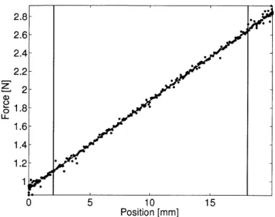
4-4 Data from a preliminary test to determine the static yield stress with

a 60 volt field and a 4.2N normal force. . . . . 50

4-5 Yield stress versus voltage for the preliminary testing along with a

linear fit. . . . . 51

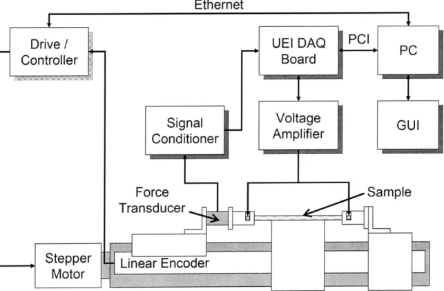
4-6 A diagram illustrating the primary components of the testing system

and how they are connected. . . . . 54

4-7 A picture of the single-axis, horizontal, linear testing system. . . . . . 55

4-8 Plot of the raw data for the 8 mm/s test and the least squares error fit. 56

4-9 Plot of the spring constant measured with the test system versus velocity. 57 4-10 Plot of the residuals of the least squares error fit to an experimental

run at 8mm/s and their frequency content. . . . . 57

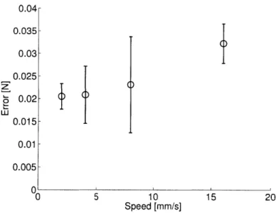
4-11 Root mean squared error of the least squares error fit versus velocity. 58

4-12 A plot of the voltage and current for five seconds with no movement

of the test stage. The frequency spectrum of the data is also shown. . 59

4-13 A plot of the error between the measured voltage and the commanded voltage versus the commanded voltage. The error bars represent one

standard deviation. . . . . 60

4-14 Plot of the root mean square of the voltage and current error, which

serves as a measure of the noise in the signal. . . . . 61

5-1 Raw force data for all three trials of variable impedance material made

with heterogeneous fluid and a kraft paper spacer for two different

testing conditions . . . . 64

5-2 Plot of the shear stress versus velocity for all voltages and materials

using heterogeneous fluid. . . . . 66

5-3 Plot of the slope and intercept of the least squares fit to the shear stress

for materials with heterogeneous fluid. . . . . 68

5-4 Plot of the mechanical work done by materials with heterogeneous fluid

5-5 Plot of the percentage increase in work done in materials with

hetero-geneous fluid at a particular voltage over the work done at OV. . . . . 73

5-6 Plot of the mean electrical energy input into the material during an

experim ental run. . . . . 74

5-7 Plot of the power density into the material during an experimental run. 75 5-8 Plot of the increase in work over the energy input for heterogeneous

m aterials. . . . . 76

5-9 Plot of the shear stress versus power density for materials with

hetero-geneous fluid. . . . . 77

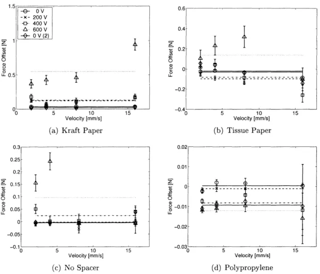
5-10 Plot of the constant force offset during the runs with heterogeneous fluid. 79

6-1 Raw force data for all three trials of variable impedance material made

with homogeneous fluid and a kraft paper spacer for two different

test-ing conditions. . . . . 82

6-2 Plot of the shear stress versus velocity for all voltages and materials

using Homogeneous fluid . . . . 83

6-3 Plot of the slope and intercept of the least squares fit to the shear stress

for materials with homogeneous fluid. . . . . 84

6-4 Plot of the mechanical work done by materials with homogeneous fluid

during the experimental run. . . . . 88

6-5 Plot of the percentage increase in work done in materials with

Homo-geneous fluid at a particular voltage over the work done at OV. . . . . 89

6-6 Plot of the mean electrical energy input into the material during an

experim ental run. . . . . 90

6-7 Plot of the power density into the homogeneous fluid based materials

during an experimental run. . . . . 91

6-8 Plot of the increase in work over the energy input for homogeneous

m aterials. . . . . 92

6-9 Plot of the shear stress versus power density for materials with

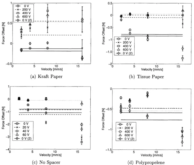
6-10 Plot of the constant force offset during the runs with Homogeneous fluid. 94

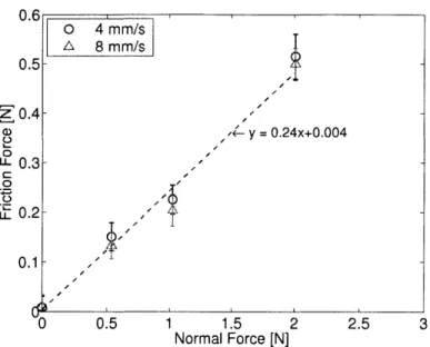
7-1 Force due to friction versus normal load for dry material. . . . . 96

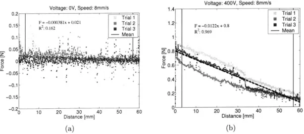
7-2 Raw data for the dry material voltage response experiment at OV and

400V . . . . . 97

7-3 Shear stress of the dry material versus velocity for four different voltages. 98

7-4 Friction term, c, in the general model versus the voltage for the dry

m aterial. . . . . 99

7-5 Work done by the dry material. . . . . 100 7-6 Percentage increase in the work done by the material over the work

done at OV. ... ... 101

7-7 Electrical energy input into the dry material. . . . . 102

7-8 Density of the electrical power going into the dry material. . . . . 102

7-9 Increase in output work divided by the input energy for dry material. 103 7-10 Shear stress of the material versus the electrical power density. . . . . 104

7-11 Force offset for the dry material . . . 104

8-1 Plot of the film thickness versus voltage for heterogeneous ERF materials. 106

8-2 Plot of the work versus normal force for heterogeneous ERF materials. 108 8-3 Plot of the shear stress versus normal force for heterogeneous ERF

m aterials. . . . . 109

8-4 Plot of the offset force versus the normal force for heterogeneous ERF

m aterials. . . . . 110

8-5 Effective coefficient of friction for the different materials with

hetero-geneous ERF. . . . .111

8-6 Plot of the work versus normal force for homogeneous ERF materials. 112 8-7 Diagram of a possible method for creating a continuous material using

sandwich geom etry. . . . . 117

A-1 Diagram of the simulink model to find the amount of energy absorbed by the m aterial. . . . 120

A-2 Final velocity of the mass after interacting with the variable impedance

material versus its initial velocity and the applied voltage. . . . .

A-3 Final velocity of the mass with model fit. . . . .

A-4 Energy absorbed by the material versus the initial velocity. . . . . B-i Raw data for experimental runs using heterogeneous fluid with a kraft

paper spacer at 0 volts. . . . . B-2 Raw data for experimental

paper spacer at 200 volts. B-3 Raw data for experimental

paper spacer at 400 volts. B-4 Raw data for experimental

paper spacer at 600 volts. B-5 Raw data for experimental

paper spacer at 0 volts. . . B-6 Raw data for experimental

paper spacer at 200 volts.

runs using heterogeneous fluid with a kraft

. . . .

runs using heterogeneous fluid with a kraft

. . . .I .

runs using heterogeneous fluid with a kraft

. . .. . . .

runs using heterogeneous fluid with a tissue

. . . .

runs using heterogeneous fluid with a tissue

125

126

127

128

. . . . 1 2 9 B-7 Raw data for experimental runs using heterogeneous fluid with a tissue

paper spacer at 400 volts. . . . . B-8 Raw data for experimental runs using heterogeneous fluid with a tissue paper spacer at 600 volts. . . . . B-9 Raw data for experimental runs using heterogeneous fluid with no

spacer at 0 volts. . . . . B-10 Raw data for experimental runs using heterogeneous fluid with no

spacer at 20 volts. . . . . B-11 Raw data for experimental runs using heterogeneous fluid with no

spacer at 40 volts. . . . . B-12 Raw data for experimental runs using heterogeneous fluid with no

spacer at 60 volts. . . . . 130 131 132 133 134 135 120 121 122 124

B-13 Raw data for experimental runs using heterogeneous fluid with a PPL spacer at 0 volts. . . . . B-14 Raw data for experimental runs using heterogeneous fluid with a PPL

spacer at 200 volts. . . . . B-15 Raw data for experimental runs using heterogeneous fluid with a PPL

spacer at 400 volts. . . . . B-16 Raw data for experimental runs using heterogeneous fluid with a PPL

spacer at 600 volts. . . . .

C-1 Raw data for experimental runs using homogeneous fluid with a kraft

paper spacer at 0 volts. . . . .

C-2 Raw data for experimental runs using homogeneous fluid with a kraft

paper spacer at 200 volts. . . . .

C-3 Raw data for experimental runs using homogeneous fluid with a kraft

paper spacer at 400 volts. . . . . C-4 Raw data for experimental runs using homogeneous fluid with a kraft

paper spacer at 600 volts. . . . .

C-5 Raw data for experimental runs using homogeneous fluid with a tissue

paper spacer at 0 volts. . . . .

C-6 Raw data for experimental runs using homogeneous fluid with a tissue

paper spacer at 200 volts. . . . .

C-7 Raw data for experimental runs using homogeneous fluid with a tissue

paper spacer at 400 volts. . . . .

C-8 Raw data for experimental runs using homogeneous fluid with a tissue

paper spacer at 600 volts. . . . .

C-9 Raw data for experimental runs using homogeneous fluid with no spacer

at 0 volts. . . . .

C-10 Raw data for experimental runs using homogeneous fluid with no spacer

at 20 volts. . . . . 136 137 138 139 142 143 144 145 146 147 148 149 150 151

C-II Raw data for experimental runs using homogeneous fluid with no spacer

at 40 volts. . . . . 152

C-12 Raw data for experimental runs using homogeneous fluid with no spacer

at 60 volts. . . . . 153

C-13 Raw data for experimental runs using homogeneous fluid with a PPL

spacer at 0 volts. . . . . 154

C-14 Raw data for experimental runs using homogeneous fluid with a PPL

spacer at 200 volts. . . . . 155

C-15 Raw data for experimental runs using homogeneous fluid with a PPL

spacer at 400 volts. . . . . 156

C-16 Raw data for experimental runs using homogeneous fluid with a PPL

spacer at 600 volts. . . . . 157

D-1 Force versus position for the dry material at OV and 4mm/s. . . . . . 160 D-2 Force versus position for the dry material at OV and 8mm/s. . . . . . 160 D-3 Force versus position for the dry material at 200V and 4mm/s. . . . . 161

D-4 Force versus position for the dry material at 200V and 8mm/s. . . . . 161

D-5 Force versus position for the dry material at 400V and 4mm/s. . . . . 162 D-6 Force versus position for the dry material at 400V and 8mm/s. ... 162

D-7 Force versus position for the dry material at 600V and 4mm/s. ... 163

Chapter 1

Introduction

1.1

Material Description

A variable-impedance material has properties, such as stiffness and damping, that

can be changed in use. Semi-active means that it requires some energy to change the properties, but no net work is done by the device. The goal is to create a material that can be worn and interact with the wearer to provide variable mechanical impedance. Some important qualities for this material include having a fast response time and low power requirement, being thin and light, and being capable of a significant change in mechanical properties.

1.2

Military Applications

The larger goal is to create a wearable "armor" that can be selectively activated depending on the threat level to allow maximum mobility while maintaining adequate protection. This would ideally be a continuous material that could be integrated into a soldier's uniform.

The shorter term goals are to engineer specific devices with particular applications in mind. One possibility is a splint that could be automatically activated when the wearer fractures a bone or sprains a joint to provide support for the impaired limb and allow the soldier to continue to function until more advanced care can be administered.

Another possibility is incorporating the material into foot and leg wear to provide variable ankle support. A common injury among paratroopers is ankle damage upon impact with the ground. To combat this, paratroopers are forced to wear bulky braces which can get caught in the parachute and require removal once on the ground. In-stead, the soldiers could wear a brace made of the variable impedance material which would be completely unobtrusive and could simply be switched off or automatically deactivate once the paratrooper is safely on the ground.

The vibration damping properties could potentially be employed to help improve aim by stabilizing a wearer's arm. Or it could be added to the butt of a rifle to reduce transmitted movements from wearer caused by things like breathing and heart beat.

1.3

Other Applications

A variable-impedance material has a wealth of non-military applications as well.

De-vices developed for the military could be readily applied to sports, with applications such as padding for football or variable ankle support for cross-training. Imagine having a ski boot that allows you to change the stiffness so you can walk normally when you are not skiing.

Other possibilities include incorporating the material into haptic devices, provid-ing feedback in a glove, for example, to simulate touchprovid-ing a surface.

1.4

Thesis Scope

This thesis is a preliminary investigation into the design of a variable-impedance material. Specifically it investigates using electrorheological (ER) fluid, a type of field-activated fluid, in creating such a material. Possible methods for using the fluid to create the material are briefly explored, but focus is placed on one particular design to determine the important factors in the design process. The goal is to begin to assess the feasibility of creating such a material and compare different methods of fabrication. We hope to come up with a method for comparing three different types

of field activated fluids: electrorheological, magnetorheological, and shear thickening to determine what applications they are best suited for.

Chapter 2 gives an introduction to field activated fluids and explains their prop-erties. Two types of ER fluids, heterogeneous and homogeneous, are described in detail.

Chapter 3 describes several possible designs for the material and models the be-havior of the design being investigated.

Chapter 4 describes the testing that was carried out on the material including the design of a unique testing system.

Chapter 5 presents the analysis methods and gives an overview of all the testing data for the materials that use heterogeneous ER fluid.

Chapter 6 examines the results of the materials that use homogeneous ER fluid.

Chapter 7 explores the properties of the same materials without any fluid in them

for comparison.

Finally, Chapter 8 discusses what can be learned from the test results and proposes future work in the area.

Chapter 2

Background

Field activated fluids have rheological properties (viscosity, yield stress, shear

mod-ulus, etc.) that change upon application of an external field. The primary types

are: shear-thickening (ST) fluid, magnetorheological (MR) fluid, and electrorheolog-ical (ER) fluid. An overall comparison of the different fluid properties is presented in Table 2 (these are values of representative fluids only, the actual fluid parameters can vary over a wide range).

2.1

Shear-Thickening Fluid

This type of fluid is characterized by a sudden increase in viscosity with increasing shear rate. At low shear rates, the fluid behaves as a liquid, but once the shear rate is increases beyond a critical value, the fluid locks up into a solid-like state. When

Property ST MR Heterogneous ER Homogeneous ER

Density (g/ml) 2 2-4 1 0.8

Viscosity (Pa-s) 1 0.1 0.1 10

Shear Stress (kPa) >10 30 4 8

Response Time (ms) <1 <10 <2 10-80

Temperature Range (C) -10-150 -40-130 -50-150 0-60

the shear stress is removed, the fluid returns to its initial liquid behavior.

This phenomenon occurs in colloidal suspensions, such as corn starch in water, and is due to the formation of particle clusters, called "hydroclusters," from the

hydrodynamic lubrication forces between particles

[6,

transition from liquid to solid has been shown to be on the order of a millisecond or less [3, 24, 21].

ST fluid has been used in damping and control devices because of its natural

rate-limiting feature [22, 13]. Lee, et al. have shown that impregnating ST fluid in Kevlar can improve the energy absorption of Kevlar fabric which has the potential to make body armor thinner and more flexible [23].

2.2

MR Fluid

Magnetorheological fluids exhibit controllable rheological behavior upon application of an external magnetic field. The apparent viscosity increases by more that two orders of magnitude in a moderate field [2].

MR fluids consist of ferromagnetic dispersed particles with a diameter on the order of one micron in a carrying fluid, such as silicone oil. Stabilizers are also often added to prevent settling or agglomeration of the particles. A magnetic field polarizes the particles and causes chains and structures to form, generating a yield stress in the fluid. Experimental evidence has shown that the yield stress is generally proportional to the square of the magnetic field strength [8].

While they were discovered at nearly the same time, MR fluids have not been researched as extensively as ER fluids. Yet they have recently found more success in commercial applications. Some examples of applications include an MR fluid brake in the exercise industry, a controllable MR fluid damper for use in truck seat suspensions

and an MR fluid shock absorber for automobile racing [17]. Some advantages of

MR fluid, especially in automotive applications, include a high shear stress, large temperature range, and low voltage requirement [2].

(a) Heterogeneous (b) Homogeneous

Figure 2-1: SEM pictures of heterogeneous and homogeneous ER fluid show the micron sized particles in heterogeneous fluid, whereas the homogeneous fluid is still continuous at this scale. Both samples were dried for an hour in a vacuum oven before placed in the SEM. The darker, textured sections of the homogeneous fluid picture

are the conductive tape on the sample holder, not part of the fluid.

2.3

ER Fluid

Electrorheological fluid quickly and reversibly changes its rheological properties in response to an electric field. There are two primary types of ER fluid: heterogeneous and homogeneous. Heterogeneous fluid, shown in Fig. 2-1(a), has solid particles suspended in a fluid medium, while homogeneous fluid, shown in Fig. 2-1(b), is a continuous liquid [20]. Both fluids are described in greater detail in the following sections.

2.3.1

Heterogeneous

Description

Heterogeneous ER fluid is the most common type of ER fluid. It was first discovered

by Winslow in 1949 and consists of micron-sized dielectric particles dispersed in an

insulating fluid medium. Upon application of a field, a yield stress develops in the fluid as the particles form chains and structures. So the fluid reversibly transforms from a liquid to a Bingham plastic, or gel, under an electric field.

Models

Several different mechanisms for the origin of the ER response have been suggested, including: degradations of the fibrous structure formed by polarization forces between particles, distortion and overlap of the electric double layers of colloidal particles re-sulting in increased energy dissipation, interelectrode circulation of particles, and the existence of water bridges between particles[19, 4]. The polarization model is generally accepted as the primary component of the ER effect. Marshall, et al. demonstrated that the relative suspension viscosity, defined as the apparent viscosity of the elec-trified suspension divided by that of the continuous phase is a function of only the

Mason number, Mn, defined as:

Mn= C (2.1)

2EoEc# 2E2

where 1c is the viscosity of the continuous phase, ' is the shear rate of the suspension, E is the magnitude of the applied electric field, co and c, are the dielectric constants

of free space and the continuous phase, respectively, and 0 = (-EC)

/

EP is the dielectric constant of the particle phase. The Mason number is a ratio of the

viscous shear forces to the electric polarization forces acting on the particles in the system, implying that these forces dominate other forces acting on the particles (van der Waals, electrostatic, and thermal)[25].

In general, ER fluid can be characterized as a Bingham plastic with a shear stress defined as:

T = Ty + T7o (2.2)

where Ty is the dynamic yield stress as shown in Fig. 2-2(a). The ER fluid also has a

static yield stress defined as the minimum shear stress required to cause the ER fluid to flow. In general, these two yield stresses are not the same[5].

The polarization model predicts that the dynamic yield stress scales as the square of the applied electric field and a variety of ER suspensions have been shown to have this behavior[1O]. However, other suspensions have shown a linear dependence on

field strength[18, 19]. Choi found that for microencapsulated polyaniline-based ER

fluid, the yield stress is proportional to E2 _{at low field strengths and approaches E}3_/2

at high field strengths[7]. To preserve generality, we describe the relationship between field strength and yield stress as:

Ty = fpE" (2.3)

where

fp

Performance Factors

Many different parameters affect the performance of heterogeneous ER fluid including

particle size, size distribution, volume fraction, particle composition, and additives. Particles in ER fluid are generally 0.1 to 100pm. At smaller particle sizes, it is

thought that the Brownian motion will compete with electrical forces to disrupt the ER effect. Larger particles would have a slow response and would be more prone

to settling under the influence of gravity [18]. Experimental results show no

mono-tonic relationship between the ER effect and the particle size. A molecular-dynamics

simulation predicts that the shear stress should be proportional to the cube of the particle diameter [30]. When two different size particles were mixed, the shear stress was found to decrease both theoretically and experimentally [35, 26].

Based on the polarization model, the yield stress increases with both volume fraction and the dielectric ratio between the particles and fluid [19]. Using a

mi-crostructural model to relate the yield stress to the electrostatic energy, Bonnecaze

et al. predict a maximum yield stress at a volume fraction of 40% for dielectric ratios less than 10 [5].

The particle composition ranges from silicates to conductive polymers to

carbona-ceous materials. Before 1985, almost all ER fluids contained a small amount of water

adsorbed on the particle surface. Many of the shortcomings associated with ER fluid were due to the presence of water, such as limited temperature range, high current

or anhydrous, ER fluids often with water chemically bonded or crystallized in the molecule. A good anhydrous ER fluid has a yield stress around 5kPa with a field

strength of 2kV/mm, a current density less than 2OptA/cm2, a temperature range

from -30 to 120*C, and a response time less than ims.

There is still room for improvement in the design of ER fluids. Zhang et al. recently fabricated a fluid using surface modified complex strontium titanate par-ticles in silicone oil with a volume fraction of 36% and measured a yield stress of 27kPa in a DC field of 3kV/mm. The conductivity at room temperature was only a

few puA/cm2_{[37]. This five to ten time increase in yield stress could open up many}

possible applications that were previously infeasable.

2.3.2

Homogeneous

Description

Homogeneous ER fluid, unlike heterogeneous ER fluid, has no solid phase. It can consist of polar liquids, nonpolar liquids, low molecular weight liquid crystals, or lyotropic polymeric liquid crystals [14, 15, 28, 11, 36]. Inoue has had particular success using side-chain type liquid crystal polymers diluted with dimethylsiloxane [16].

In immiscible liquid blends, such as the liquid crystal polymer in solution, the electric field causes the viscous droplets to elongate and bridge across the electrodes. With no field, the viscosity is comparable to the low viscosity solution and at high fields the viscosity is comparable to that of the LCP forming the bridges [29].

Homogeneous fluids don't suffer from the disadvantages in heterogeneous fluid such as particle settling, agglomeration and abrasion. They also may be more suited to scaling down to smaller sizes because they are still homogeneous at micron scales while heterogeneous fluid has solid particles at this scale.

Model

While some fluids such as solutions of poly(-benzoyl-L-glutamate) in dioxane and dichloroethane exhibit a yield stress varying with field strength just like heterogeneous

E CO Shear Rate [s-1] (a) Heterogeneous E Shear Rate [s-1] (b) Homogeneous

Figure 2-2: The characteristic shear stress versus shear rate for both heterogeneous and homogeneous ER fluid. The heterogeneous ER fluid develops a yield stress with increasing field strength, while the viscosity remains constant. The homogeneous ER fluid has an increasing viscosity with field strength.

fluids [16], the majority of homogeneous ER fluids have a viscosity that increases with field strength and no yield stress as shown in Fig. 2-2(b). There is no well defined relationship between the viscosity and the field strength, but assuming a power law relationship,the shear stress can be expressed as:

T = (ro + fcE n)§ (2.4)

where the initial fluid viscosity is increased with the electric field. The parameter

f,

Chapter 3

Material Design

In this chapter, an initial design of the variable impedance material is presented.

3.1

Force Transmission

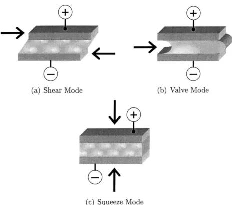
To create a material with variable properties, we need a method for translating the change in fluid properties to mechanical properties such as stiffness and damping. There are three primary modes of force transmission in field-activated fluids: shear, valve and squeeze mode, illustrated in Figure 3-1.

3.1.1

Shear

In shear mode, the force is transmitted orthogonal to the field by resisting the motion of the top and bottom bounding plates. This mode is used in applications such as clutches and brakes where two concentric cylinders, with fluid in between, are rotated with respect to each other. The amount of torque transmitted from one cylinder to the other is determined by the field strength.

3.1.2

Valve

In valve mode, the field strength determines the amount of pressure drop that may be supported through the electrode gap. This mode is used in piston and cylinder

Q

(a) Shear Mode

4,

(b) Valve Mode

Q

() T

(c) Squeeze Mode

Figure 3-1: These figures illustrate the three mechanisms of force transmission for a field-activated fluid.

dampers where the resistance to flow, and hence damping, are controlled by the field strength.

3.1.3

Squeeze

Finally, in squeeze mode, force is transmitted parallel to the field as the fluid thickness changes. Compression-type dampers employ this mode of force transmission.

3.2

Geometry

This thesis is an investigation into using field activated fluids to create a thin variable impedance material. How can we use these force transmission methods in a thin flexible material? Three different design ideas were considered: channel, grid, and sandwich. Each of these geometries can be used for all three field-activated fluids, but specific implementations using ER fluid are presented.

I

I

'

II

+

Figure 3-2: Illustration of the channel design for an electrorheological fluid based variable impedance material. The alternating electrodes would create a pressure difference between two resevoirs of ER fluid.

3.2.1

Channel

A channel geometry exploits the valve mode of force transmission. The general idea

is for macro-scale material deformation to cause the flow of fluid through narrow channels. The flow through the channels can be regulated by applying a field, thus

regulating the overall material properties.

One possible implementation of the channel geometry using ER fluids is depicted in Fig. 3-2. Alternating electrodes, with layers above and below as seals, confine the fluid to narrow pathways. Bending perpendicular to the channel direction would tend to cause fluid flow, like squeezing toothpaste out of the tube. By applying a voltage across the electrodes, resistance to flow is increased, and thus increasing the resistance to bending. Alternating layers could be oriented in different directions, like in a laminar fiber composite, to control bending in a variety of directions.

Another implementation of this geometry is to fill hollow fibers with the fluid which could then be woven into a continuous fabric. This would create a material similar to a traditional textile but with the possibility of some control over its mechanical properties.

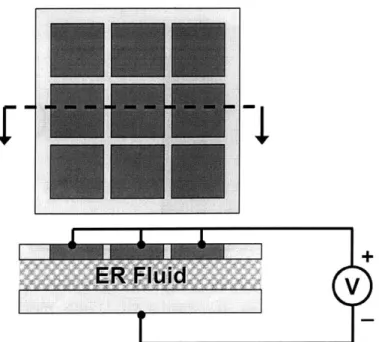
Figure 3-3: An illustration of a possible grid type design of an electrorheological fluid based variable impedance material.

3.2.2

Grid

In a grid geometry, there are two flexible layers with the fluid in between. By dividing up the sheet into discrete areas where field can be applied, the material can be selectively controlled. An implementation using ER fluid is shown in Fig. 3-3. There are electrodes above and below the fluid. The bottom electrode is continuous, but the top one is broken into squares so that each one can be adjusted independently.

Taylor, et al. created a similar grid, but with a rigid bottom to act as a haptic display device. By activating different areas, they could create different textures on the top flexible electrode made of conducting rubber. Running a roller across the surface, they measured vertical forces up to 150 grams of force when moving from an inactive cell to an active cell [31, 32].

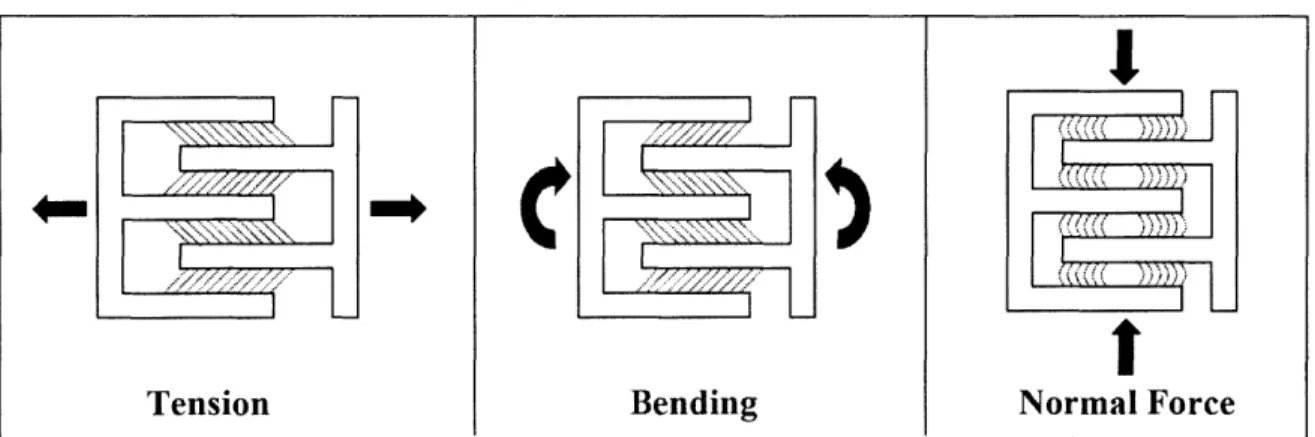
3.2.3

Sandwich

The third type of geometry involves stacking multiple flexible layers with the fluid in between them, attaching opposite layers at opposite ends. Figure 3-4 illustrates how pulling the ends apart involves the shear mode of force transmission as does bending

'I

Tension Bending Normal Force

Figure 3-4: Three different loading conditions on a sandwich geometry illustrating the variety of force transmission methods that can be utilized.

the sample. Applying a normal force tends to cause fluid flow and therefore the valve mode of transmission can be exploited.

For an ER fluid, each layer would be an electrode, with the voltage applied at opposite ends. Because there are multiple thin layers, the distance between adjacent electrodes is small, so a low voltage could provide a very high field strength to the fluid. In order to prevent the adjacent electrodes from contacting, a spacer is added between each electrode.

3.3

Design Considerations

The material design, whether it involves one or all of these three geometries, will involve design considerations which are common to all three geometries.

3.3.1

Size

The material must be thin, so it becomes important to understand how these fluids behave in small spaces. Typical devices have gaps on the order of millimeters; the new material will have gaps on the order of microns or less. We would like to understand the scaling laws that determine how the properties of the material behave as the size is reduced.

3.3.2

Flexible Boundary Conditions

The material must also be flexible to allow freedom of movement which creates the unique situation of unconstrained boundary layers. The distance between the layers is not rigidly fixed as it is in most applications so the thickness between the electrodes can vary over time and also over position.

3.3.3

Arbitrary Loading

As it is worn by a human, the material could be subjected to a variety of loading conditions. For example, the material could be stretched and bent around a joint at the same time a normal force is applied from an impact.

3.3.4

Failure Modes

It is also important to understand the primary mechanisms for material failure. In ER fluid based materials, electrical breakdown is a likely candidate. The flexible electrodes combined with arbitrary loading mean the electrode gap could become quite small in local areas, resulting in dielectric breakdown. Adding the spacer may help reduce the risk of failure by preventing the electrodes from coming too close together. However, there may be an advantage to scaling down the space between electrodes. Paschens law, which relates the breakdown strength to the product of the gap spacing and pressure, predicts the breakdown strength of air at atmospheric pressure reaches a minimum around 4ptm and then increases as the distance becomes smaller. But recent work indicates the breakdown strength of air actually continues to decrease below 4pm [33].

3.4

Shear Model

As a preliminary effort to gain insight into some of these design criteria, we intend to model a simple implementation of the variable impedance material and then compare the model to experimental results. Since the shear mode of force transmission is

Mylar Aluminum

F L Spacer

;' ER Fluid

tf te

Figure 3-5: Illustration of the basic shear stress loading condition. The thickness of

the fluid film is tf and the distance between the electrodes is te.

well understood in traditional ER fluid applications, it will be investigated using a sandwich-type geometry. Without a loss of generality, the geometry can be reduced to a single layer of fluid with electrodes on the top and bottom and a spacer in the middle. The force in tension on the sample, which translates to a shear stress on the fluid, is measured by holding one side fixed while the other is moved as shown in

Fig. 3-5.

To model the behavior of this material the basic fluid models discussed in Chap-ter 2 will be used. Any discrepancies in the results will help bring out some of the

unique features of this material. The shear force, F, is given by:

F = AT (3.1)

Where A is the area where the two electrodes overlap. For this configuration, the area is given by:

A = w(L - x) (3.2)

where w is the width of the layer, L is the initial length of the overlapping area, and

x is the displacement of the top layer. Combining the previous two equations, we find

that the shear stress is linear with respect to position:

So we expect the shear force to start out as a maximum and then decrease to zero when x equals L. Note that this model is assuming the material is loaded in tension and is therefore only valid when x > 0.

If we assume that the dielectric constant between the electrodes is uniform, the

field strength is simply the applied voltage divided by the distance between the elec-trodes:

E = - (3.4)

te

where te is the distance between the electrodes and V is the applied voltage.

Further-more, the shear rate is defined as the velocity of the top layer divided by the fluid thickness:

(3.5) tf

where tf is the thickness of the fluid layer and ± is the velocity.

3.4.1

Heterogeneous ER Fluid

We can combine Equations 2.2, 2.3, 3.4, and 3.5 to find the shear stress in the material with heterogeneous fluid:

4 f=

- V _(3.6)

tf ten

3.4.2

Homogeneous ER Fluid

Likewise, for the homogeneous fluid, using Equation 2.4 gives:

7o= + fcV%

(3.7)

tf _tntf

3.4.3

Electrostatics

In addition to the standard fluid models, the flexible electrodes will experience elec-trostatic forces similar to a parallel plate capacitor.The effective capacitance of the sandwich is given by:

C = rOA (3.8)

Assuming the electrodes form an infinite parallel plate capacitor (ignoring edge effects), the normal force pulling the two electrodes together is given by:

Fn = 2 V2 (3.9)

where K is the dielectric constant of the material between the electrodes, co is the

permittivity of free space (8.854 x 10 1 2_{F/m). While the standard fluid model is not}

directly affected by a normal force in the standard configuration, the normal force may have an indirect effect by changing the thickness.

The force required to slide the electrodes apart based solely on the capacitor model (ignoring the fluid) is given by:

Fx = KEOWV2 (3.10)

2te

This equation is derived by differentiating the energy stored in a capacitor:

U = Kf"wV2 (L - x) (3.11)

2te

with respect to displacement, x. Since this force does not depend on position, it will add a constant offset to the shear force prediction. The importance of this term is not readily calculable; it depends on material properties as well as applied voltage, speed and position. It will be assumed to be negligible in forming the model, but will be kept in mind as a possible explanation for discrepancies between the model and

experiment.

3.4.4

Dry Material

The voltage dependent normal force found in the previous section implies that the

shear force could be controlled using simple Coulomb friction. The dry material behaves as follows:

T /_tKEOV 2 (3.12)

Where P is the coefficient of kinetic friction between the spacer and the electrode. It is worth noting that even without an ER fluid the sandwich material still exhibits a shear stress that is voltage dependent. This reveals an alternate method for creating this variable-impedance material other than field activated fluids and has the possibility of saving weight. Because it has the same geometry, it could also be used in addition to field activated fluid based material. This electrostatic induced friction is known as the Johnsen-Rahbek effect and was investigated in the mid 50s at IBM for creating a clutch with fast response time [9].

3.4.5

General Model

The three models presented previously (heterogeneous, homogeneous, and dry ma-terial) have similar properties that allow them all to be represented by one general model to facilitate comparisons between the materials. The homogeneous fluid acts like a voltage dependent damper, while the dry and heterogeneous fluids act like volt-age dependent Coulomb friction. Thus the general model is represented as a voltvolt-age dependent damper and voltage dependent Coulomb friction in series. The shear stress is given as:

T- c(V) + b(V)X (3.13)

Where c and b are the Coulomb friction and damping coefficients, respectively. Using the fluid models, the shear stress can be expanded to:

T = (ao + aVn) + (a2 + a3 Vn 2_{)± (3.14)} Material ao a, a2 a3 ni n2 Heterogeneous Fluid 0 - 0 1-2 0 Homogeneous Fluid 0 0 70 0-2 Dry 0 O 0 0 2 0

Table 3.1: Parameters for general model in terms of material properties.

proper-ties for all three types of material is shown in Table 3.1. Notice that ao is zero for all models, indicating that none of the models predict a friction force at zero field strength. This term was added in to provide symmetry and to verify that it actually

is zero rather than assuming it is. Also note that both ni and n2 are not well

un-derstood with relation to the material properties and can only be determined from empirical data.

3.5

Performance Analysis

With the models for shear stress established, it is useful to come up with a measure for overall material performance to help compare the different fluids. In general, we would like to use this material to help abosrb a controllable amount of energy, so looking at the amount of energy absorbed by this material as it is pulled apart is helpful. One method for estimating the energy absorption is to compute the work done in pulling the layers apart at a constant velocity, which approximates the mechanism for preventing joint motion. Another approach is to look at the amount of energy that can be absorbed from a mass with some initial kinetic energy, which approximates the absorption of an impact. Both of these measures are examined in two different geometrical configurations.

3.5.1

Parallel Loading

In this configuration, the force is applied parallel to the sample, causing the layers to remain horizontal while being pulled apart. This is the same condition as the one shown in Fig. 3-5, and the model equations derived previously all apply. In this case the work done at a constant velocity is given by:

W = Fdx (3.15)

L

W j Tw(L--x)dx (3.16)

where a = wL 2_{/2. So the total work, which is equivalent to the energy absorbed, is}

proportional to the shear stress for a given geometry.

The more interesting problem is to determine how much energy would be absorbed

by the material if a given mass, M, with initial energy, EO = 1/2M±2 was attached

to the end of the sample. The force exerted by the sample will slow down the mass until either the mass comes to a complete stop or the layers separate. The dynamic equation for the mass is given by:

M .. c(V)L + b(V)Li - c(V)x - b(V)x, W X 0 (± > 0, x

(<

to solve the differential equation, mass can be approximated as:

as shown in Appendix A, the

.0

Xf =

{0O

- 2 (c(V) _{+ b(V))}

In some cases the final velocity drops to zero, meaning all the absorbed by the material. This occurs when the initial velocity

initial velocity, ,Oc, which is given by:

initial energy was

is below a critical

Xoc = ₂Mb(V) + c(V) + b(V)

Written in terms of the critical initial energy instead of velocity gives:

Sb(V) c(V)

Eoc = 2-c(V) +± _{(2-b(V)) + 2bV C()+(2 V)}

(3.20)

(3.21)

This is the amount of initial energy that can be totally absorbed by the material. Be-cause force is applied only when the layers are in contact, the critical absorbed energy depends on the mass of the object being stopped, not just the material properties.

(±o -Oc)

(±O

F

be.Iv.

LS

x

D

Figure 3-6: Diagram illustrating the perpendicular loading condition where the ma-terial is pinned on either side and a force acts through the center causing the layers to slide apart.

In general, the overall energy absorbed is given by:

( ( 0 [i - 9j1~ 0~ 9 j (±0 > i0c)

ce (c(V) + b(V).,o) 2M±:' (z > -Oc)

(3.22)

Notice that as the energy becomes large, the energy absorbed approaches that pre-dicted by Eq. 3.17, which makes sense because at large energies the velocity hardly changes, matching the earlier assumption.

3.5.2

Perpendicular Loading

The perpendicular loading condition is especially suited for a ball-drop test to verify the energy absorption predictions. In this configuration, the force is exerted orthogo-nal to the length of the sample with each end of the sample pinned in place as shown in Fig. 3-6. The layers separate as the center of the sample is pushed down. If we assume that the displacement causes a triangular deformation, as indicated by the

dashed lines in the figures, the overlapping area is given by:

A = w(2Ls - V4x2 _{+ D}2_{) (3.23)}

where D is the distance between the supports and L, is the length of each strip. Note that L, is defined slightly differently than L in the parallel loading case.

Using the model presented in Eq. 3.13 and assuming the tension in the material is the shear stress times the area of overlap, the force exerted on the object is given

by:

F = 4w c(V) + 4 ₂ b(V) 2xL -x (3.24)

-v4x2 + D2 V4,2+ D2

To make the next step more clear, we first replace D with mL, where m

c

Then the work can be calculated as in the previous section by integrating the force

from x = 0 to x - -V4 -n 2, which is the point where the layers separate.

2 W = a, (Ac(V) + Bb(V)±) (3.25) where wL82 as 2 (3.26) 2 A (2 - M)2 _(3.27) B 4 -rn2 _{- 8m arctan}

(

Notice the similarity to equation 3.17. The only difference is that the damping and friction elements are weighted differently depending on the initial geometry. For M = 1, which means that the layers begin completely overlapped (and L, becomes

equivalent to the L in the parallel case), A = 1 and B ~ 1.18. So in this case, the

effect of the damping element is increased 18% with a corresponding increase in the overall work done by the material.

differential equation:

4x1 x

M 2 = 4w c(V) + 4x b(V)

(

V4x2 + D2 ) /4X2 + D 2

This equation can be simulated to find the approximate final velocity of the mass, as in the previous section. Using this final velocity, the total amount of energy absorbed

by the material is given by:

Ea 4 a Ac(V)JBb v) G ( -4c) (3.30)

a.

+

where the critical initial velocity, boc is given by:

X c = 8 Bb(V) + - Ac(V ) + Bb(V) (3.31)

2M M (2M

With these equations, the energy absorption behavior of a material can be pre-dicted after finding the model parameters. As an illustrative example, if the material was used in an ankle brace, the energy and mass of a falling human body could be used to find the voltage necessary to absorb enough energy to prevent ankle injury when the wearer's feet hit the ground.

Chapter 4

Testing

4.1

Preliminary Testing

To make sure that the sandwich geometry does in fact have a voltage dependent shear stress, a preliminary test was first carried out. The goal was to examine how ER fluid behaves in the thin film necessary for incorporation into a uniform and how the properties of the fluid translate into macroscopic properties.

The first prototype employed a simple sandwich design resembling a parallel plate capacitor. The ER fluid was contained between two electrode plates along with an insulator that prevented the electrodes from contacting and shorting.

A schematic of the layers in the prototype is shown in Figure 4-1. The electrodes

were made with aluminum foil, 20 microns thick. The insulator was tissue paper, 30 microns thick. The ER fluid used was manufactured by Bridgestone (F569HT), but is no longer commercially available. It consisted of carbonaceous particles 1-10 microns

in diameter in silicone oil with a 67% solid volume fraction [271. The electrorheological

properties of the ER fluid were not measured directly, but it was reported to have a shear yield stress of 4kPa at a field strength of 4kV/mm.

The prototype was constructed by affixing the bottom foil and paper layer to a plastic block with an adhesive. The paper was then coated with the ER fluid and another foil layer was placed on top. Finally, a layer of polypropylene was glued to the top layer of foil for insulation. Electrical connection was made by attaching alligator

Paper

Foil

Figure 4-1: Schematic of the prototype Figure 4-2: Picture of the prototype on the

material consisting of a layer of paper sat- block used for the shear test. The electrical

urated in ER fluid and surrounded by two connections are made on opposite sides of

layers of aluminum foil. the sample using alligator clips.

clips to opposite ends of the two foil layers as shown in Figure 4-2. The spacing between the two electrodes was estimated to be 0.1 mm by measuring the thickness of the paper coated with ER fluid. It should be noted that the fluid was absorbed by the paper layer and was present on both sides of the paper. It was unclear, however, if the particles in the ER fluid were absorbed into or through the paper.

4.1.1

Test Description

One of the fundamental characteristics of heterogeneous ER fluid is the variation in shear yield stress with applied electric field. Thus, the shear yield stress of the prototype material should have an observable dependence on field strength. In this experiment, the static yield stress, which is the value of stress beyond which the material undergoes free deformation, was measured.

To determine the static yield stress of the material, a plate was attached to the top of the prototype and a six-axis force transducer was attached to the plate such that the X and Y axes were on the same plane as the material as shown in Figure 4-3. Using a spring as an aid, a force ramp was manually applied to the force transducer until an observable displacement of about 5mm occurred. During the test, the X, Y, and Z channels of the force transducer were recorded on a computer at a sampling rate of 1kHz. The test was repeated three times with each of the following voltages